Propagation of localized optical waves in media with dispersion, in dispersionless media and in vacuum. Low diffractive regime

Abstract

We present a systematic study on linear propagation of ultrashort laser pulses in media with dispersion, dispersionless media and vacuum. The applied method of amplitude envelopes gives the opportunity to estimate the limits of slowly warring amplitude approximation and to describe an amplitude integro-differential equation, governing the propagation of optical pulses in single cycle regime. The well known slowly varying amplitude equation and the amplitude equation for vacuum are written in dimensionless form. Three parameters are obtained defining different linear regimes of the optical pulses evolution. In contrast to previous studies we demonstrate that in femtosecond region the nonparaxial terms are not small and can dominate over transverse Laplacian. The normalized amplitude nonparaxial equations are solved using the method of Fourier transforms. Fundamental solutions with spectral kernels different from Fresnel one are found. One unexpected new result is the relative stability of light pulses with spherical and spheroidal spatial form, when we compare their transverse enlargement with the paraxial diffraction of lights beam in air. It is important to emphasize here the case of light disks, i.e. pulses whose longitudinal size is small with respect to the transverse one, which in some partial cases are practically diffractionless over distances of thousand kilometers. A new formula which calculates the diffraction length of optical pulses is suggested.

1 Introduction

For long time few picosecond or femtosecond (fs) optical pulses with approximately equal duration in the $x$, $y$ and $z$ directions (Light Bullets or LB), and fs optical pulses with relatively large transverse and small longitudinal size (Light Disks or LD) are used in the experiments. The evolution of so generated LB and LD in linear or nonlinear regime is quite different from the propagation of light beams and they have drawn the researchers’ attention with their unexpected dynamical behavior. For example, self-channeling of femtosecond pulses with power little above the critical for self-focusing [1] and also below the nonlinear collapse threshold [2] (linear regime) in air, was observed. This is in contradiction with the well known self-focusing and diffraction of an optical beam in the frame of paraxial optics. Various unidirectional propagation equations have been suggested to be found stable pulse propagation mainly in nonlinear regime (see e.g. Moloney and Kolesik [3], Couairon and Mysyrowicz [4], Chin at all. [5], for a review). The basic studies in this field started with the so called spatio-temporal nonlinear Schrödinger equation (NSE) which is one compilation between paraxial approximation, the group velocity dispersion (GVD) and nonlinearity [6, 7, 8, 9]. The influence of additional physical effects were studied by adding different terms to this scalar model as small nonparaxiality [15, 18], plasma defocussing, multiphoton ionization and vectorial generalizations. It is not hard to see that for pulses with low intensity (linear regime) in air and gases the additional terms as GVD and others become small and the basic model can be reduced to paraxial equation. This is the reason diffraction of a low intensity optical pulse governed by this model on several diffraction length to be equal to diffraction of a laser beam. On other hand, the experimentalists have discussed for a long time that in their measurements the diffraction length of an optical pulse is not equal to this of a laser beam $z^{beam}_{diff}=k_{0}r^{2}_{\perp}$, even when additional phase effects of lens and other optical devices can be reduced. Here $k_{0}$ denotes laser wave-number and $r^{2}_{\perp}$ denotes the beam waist. Thus exist one deep difference between the existing models in linear regime, predicting paraxial behavior in gases, and the real experiments.

The purpose of this work is to perform a systematic study of linear propagation of ultrashort optical pulses in media with dispersion, dispersionless media and vacuum and to suggest a model which is more close to the experimental results. In addition, there are several particular problems under consideration in this paper.

The first one is to obtain (not slowly varying) amplitude envelope equation in media with dispersion governing the evolution of optical pulses in single-cycle regime. This problem is natural in femtosecond region where the optical period of a pulse is of order $2-3$ fsec. The earliest model for pulses in single-cycle regime suggested by Brabec and Krausz [20] is obtained after Taylor expansion of wave vector $k^{2}(\omega)$ about $\omega_{0}$. It is easy to show [21] that this expansion diverge in solids for single-cycle pulses. The higher order dispersion terms start to dominate and the series can not cut off. This is the reason more carefully and accurately to derive the envelope equation before using Taylor series. In this way we obtain an integro-differential envelope equation where no Taylor expansion of the wave vector $k^{2}(\omega)$, governing evolution of single cycle pulses in solids.

The second problem is to investigate more precisely the slowly varying envelope equations governing the evolution of optical pulses with high number of harmonics under the envelope. The slowly varying scalar Nonlinear Envelope Equation (NEE) is derived in many books and papers [11, 12, 13, 14, 15, 16, 17]. After the deriving of the NEE, most of the authors use a standard procedure to neglect the nonparaxial terms as small ones. Only some partial nonparaxial approximations in free space [10, 15, 18] and optical fibers [19] were studied. In [22] we rewrite the NEE in dimensionless form and estimate the influence of the different linear and nonlinear terms on the evolution of optical pulses. We found that both nonparaxial terms in NEE, second derivative in propagation direction and second derivative in time with $1/v^{2}$ coefficient, are not small corrections. In fs region they are of same order as transverse Laplacian or start to dominate. These equations with (not small) nonparaxial terms are solved in linear regime [22] and investigated numerically in nonlinear [23]. In this paper we include GVD term in the nonparaxial model and study also the envelope equation of electrical field in vacuum and dispersionless media. It is important to note that the Vacuum Linear Amplitude Equation (VLAE) is obtained without any expansion of the wave vector. That is why it work also for pulses in single-cycle regime (subfemto and attosecond pulses).

Last but not least the nonparaxial equations for media with dispersion, dispersionless media and vacuum are solved in linear regime and new fundamental solutions, including the GVD, are found. The solutions of these equations predict new diffraction length for optical pulses $z^{pulse}_{diff}=k_{0}^{2}r^{4}_{\perp}/z_{0}$, where $z_{0}$ is the longitudinal spatial size of the pulse (the spatial analog of the time duration $t_{0}$; $z_{0}=vt_{0}$; v is group velocity). In case of fs propagation in gases and vacuum we demonstrate by these analytical and numerical solutions a significant decreasing of the diffraction enlargement in respect to paraxial beam model and a possibility to reach practically diffraction-free regime.

2 From Maxwell’s equations of a source-free, dispersive,
nonlinear Kerr type medium to the amplitude equation

The propagation of ultra-short laser pulses in isotropic media, can be characterized by the following dependence of the polarization of first $\vec{P}_{lin}$ and third $\vec{P}_{nl}$ order on the electrical field $\vec{E}$:

$$\vec{P}_{lin}=\int\limits_{-\infty}^{t}{\left(\delta(\tau-t)+4\pi\chi^{\left(1\right)}\left(\tau-t\right)\right)\vec{E}\left(\tau,r\right)}d\tau=$$

$$\int\limits_{-\infty}^{t}{\varepsilon\left(\tau-t\right)\vec{E}\left(\tau,x,y,z\right)}d\tau,$$ (1)

$$\vec{P}_{nl}^{(3)}=3\pi\int\limits_{-\infty}^{t}\int\limits_{-\infty}^{t}\int\limits_{-\infty}^{t}\chi^{\left(3\right)}\left(\tau_{1}-t,\tau_{2}-t,\tau_{3}-t\right)$$

$$\times\left(\vec{E}(\tau_{1},r)\cdot\vec{E}^{*}(\tau_{2},r)\right)\vec{E}(\tau_{3},r)d\tau_{1}d\tau_{2}d\tau_{3},$$ (2)

where $\chi^{(1)}$ and $\varepsilon$ are the linear electric susceptibility and the dielectric constant, $\chi^{(3)}$ is the nonlinear susceptibility of third order, and we denote $r=(x,y,z)$. We use the expression of the nonlinear polarization (2), as we will investigate only linearly or only circularly polarized light and in addition we neglect the third harmonics term. The Maxwell’s equations in this case becomes:

$$\nabla\times\vec{E}=-\frac{1}{c}\frac{\partial\vec{B}}{\partial t},$$ (3)

$$\nabla\times\vec{H}=\frac{1}{c}\frac{\partial\vec{D}}{\partial t},$$ (4)

$$\nabla\cdot\vec{D}=0,$$ (5)

$$\nabla\cdot\vec{B}=\nabla\cdot\vec{H}=0,$$ (6)

$$\vec{B}=\vec{H},\ \vec{D}=\vec{P}_{lin}+\vec{P}_{nl},$$ (7)

where $\vec{E}$ and $\vec{H}$ are the electric and magnetic fields strengths, $\vec{D}$ and $\vec{B}$ are the electric and magnetic inductions. We should point out here that these equations are valid when the time duration of the optical pulses $t_{0}$ is greater than the characteristic response time of the media $\tau_{0}$ ($t_{0}>>\tau_{0}$), and also when the time duration of the pulses is of the order of time response of the media ($t_{0}\leq\tau_{0}$). Taking the curl of equation (3) and using (4) and (7), we obtain:

$$\nabla\left(\nabla\cdot\vec{E}\right)-\Delta\vec{E}=-\frac{1}{c^{2}}\frac{\partial^{2}\vec{D}}{\partial t^{2}},$$ (8)

where $\Delta\equiv\nabla^{2}$ is the Laplace operator. Equation (8) is derived without using the third Maxwell’s equation. Using equation (5) and the expression for the linear and nonlinear polarizations (2) and (2), we can estimate the second term in equation (8) for arbitrary localized vector function of the electrical field. It is not difficult to show that for localized functions in nonlinear media with and without dispersion $\nabla\cdot\vec{E}\cong 0$ and we can write equation (8) as follows:

$$\Delta\vec{E}=\frac{1}{c^{2}}\frac{\partial^{2}\vec{D}}{\partial t^{2}}.$$ (9)

We will now replace the electrical field in linear and nonlinear polarization on the right-hand side of (9) with it’s Fourier integral:

$$\vec{E}\left(r,t\right)=\int\limits_{-\infty}^{+\infty}\hat{\vec{E}}\left(r,\omega\right)\exp{\left(-i\omega t\right)}d\omega,$$ (10)

where with $\hat{\vec{E}}\left(r,\omega\right)$ we denote the time Fourier transform of the electrical field. We thus obtain:

$$\Delta\vec{E}=\frac{1}{c^{2}}\frac{\partial^{2}}{\partial t^{2}}\left(\int\limits_{-\infty}^{t}\int\limits_{-\infty}^{\infty}\varepsilon(\tau-t)\hat{\vec{E}}\left(r,\omega\right)\exp{(-i\omega\tau)}d\omega d\tau\right)+$$

(11)

$$\frac{3\pi}{c^{2}}\frac{\partial^{2}}{\partial t^{2}}\int\limits_{-\infty}^{t}\int\limits_{-\infty}^{t}\int\limits_{-\infty}^{t}\int\limits_{-\infty}^{\infty}\chi^{\left(3\right)}\left(\tau_{1}-t,\tau_{2}-t,\tau_{3}-t\right)\left|\hat{\vec{E}}\left(r,\omega\right)\right|^{2}\hat{\vec{E}}\left(r,\omega\right)$$

$$\times\exp{\left(-i\left(\omega(\tau_{1}-\tau_{2}+\tau_{3})\right)\right)}d\omega d\tau_{1}d\tau_{2}d\tau_{3}.$$

The causality principle imposes the following conditions on the response functions:

$$\varepsilon(\tau-t)=0;\ \chi^{\left(3\right)}\left(\tau_{1}-t,\tau_{2}-t,\tau_{3}-t\right)=0,$$

$$\tau-t>0;\ \tau_{i}-t>0;\ i=1,2,3.$$ (12)

That is why we can extend the upper integral boundary to infinity and use the standard Fourier transform [13]:

$$\int\limits_{-\infty}^{t}{\varepsilon(\tau-t)\exp{(-i\omega\tau)}d\tau}=\int\limits_{-\infty}^{+\infty}{\varepsilon(\tau-t)\exp{(-i\omega\tau)}d\tau},$$ (13)

$$\int\limits_{-\infty}^{t}\int\limits_{-\infty}^{t}\int\limits_{-\infty}^{t}\chi^{\left(3\right)}\left(\tau_{1}-t,\tau_{2}-t,\tau_{3}-t\right)d\tau_{1}d\tau_{2}d\tau_{3}=$$

$$\int\limits_{-\infty}^{+\infty}\int\limits_{-\infty}^{+\infty}\int\limits_{-\infty}^{+\infty}\chi^{\left(3\right)}\left(\tau_{1}-t,\tau_{2}-t,\tau_{3}-t\right)d\tau_{1}d\tau_{2}d\tau_{3}.$$ (14)

The spectral representation of the linear optical susceptibility $\hat{\varepsilon_{0}}(\omega)$ is connected to the non-stationary optical response function by the following Fourier transform:

$$\hat{\varepsilon}(\omega)\exp{(-i\omega t)}=\int\limits_{-\infty}^{+\infty}{\varepsilon(\tau-t)\exp{(-i\omega\tau)}d\tau}.$$ (15)

The expression for the spectral representation of the non-stationary nonlinear optical susceptibility $\hat{\chi}^{(3)}$ is similar :

$$\hat{\chi}^{(3)}(\omega)\exp{(-i\omega t)}=\int\limits_{-\infty}^{+\infty}\int\limits_{-\infty}^{+\infty}\int\limits_{-\infty}^{+\infty}\chi^{\left(3\right)}\left(\tau_{1}-t,\tau_{2}-t,\tau_{3}-t\right)$$

$$\times\exp{\left(-i\left(\omega(\tau_{1}-\tau_{2}+\tau_{3})\right)\right)}d\tau_{1}d\tau_{2}d\tau_{3}.$$ (16)

Thus, after brief calculations, equation (2) can be represented as

$$\Delta\vec{E}=-\int\limits_{-\infty}^{\infty}\frac{\omega^{2}\hat{\varepsilon}(\omega)}{c^{2}}\hat{\vec{E}}\left(r,\omega\right)\exp{(-i\omega t)}d\omega$$

$$+\int\limits_{-\infty}^{\infty}\frac{\omega^{2}\hat{\chi}^{\left(3\right)}\left(\omega\right)}{c^{2}}\left|\hat{\vec{E}}\left(r,\omega\right)\right|^{2}\hat{\vec{E}}\left(r,\omega\right)\exp{\left(-i\left(\omega t\right)\right)}d\omega.$$ (17)

We now define the square of the linear $k^{2}$ and the generalized nonlinear $\hat{k}_{nl}^{2}$ wave vectors, as well as the nonlinear refractive index $n_{2}$ with the expressions:

$$k^{2}=\frac{\omega^{2}\hat{\varepsilon}\left(\omega\right)}{c^{2}},$$ (18)

$$\hat{k}_{nl}^{2}=\frac{3\pi\omega^{2}\hat{\chi}^{(3)}\left(\omega\right)}{c^{2}}=k^{2}n_{2},$$ (19)

where

$$n_{2}(\omega)=\frac{3\pi\hat{\chi}^{(3)}\left(\omega\right)}{\hat{\varepsilon}\left(\omega\right)}.$$ (20)

The connection between the usual dimensionless nonlinear wave vector $k_{nl}^{2}$ and the generalized one (19) is: $k_{nl}^{2}=\hat{k}_{nl}^{2}\left|\hat{\vec{E}}\left(r,\omega\right)\right|^{2}$. In terms of these quantities, equation (2) can be expressed by:

$$\Delta\vec{E}=-\int\limits_{-\infty}^{\infty}k^{2}(\omega)\hat{\vec{E}}\left(r,\omega\right)\exp{(-i\omega t)}d\omega$$

$$-\int\limits_{-\infty}^{\infty}k^{2}(\omega)n_{2}(\omega)\left|\hat{\vec{E}}\left(r,\omega\right)\right|^{2}\hat{\vec{E}}\left(r,\omega\right)\exp{\left(-i\left(\omega t\right)\right)}d\omega.$$ (21)

Let us introduce here the amplitude function $\vec{A}(r,t)$ for the electrical field $\vec{E}(r,t)$:

$$\vec{E}\left(x,y,z,t\right)=\vec{A}\left(x,y,z,t\right)\exp{\left(i(k_{0}z-\omega_{0}t)\right)},$$ (22)

where $\omega_{0}$ and $k_{0}$ are the carrier frequency and the carrier wave number of the wave packet. The writing of the amplitude function in this form means that we consider propagation only in $+z$ -direction and neglect the opposite one. Let us write here also the Fourier transform of the amplitude function $\hat{\vec{A}}(r,\omega-\omega_{0})$:

$$\vec{A}\left(r,t\right)=\int\limits_{-\infty}^{+\infty}\hat{\vec{A}}\left(r,\omega-\omega_{0}\right)\exp{\left(-i(\omega-\omega_{0})t\right)}d\omega,$$ (23)

and the following relation between the Fourier transform of the electrical field and the Fourier transform of the amplitude function:

$$\hat{\vec{E}}\left(r,\omega\right)\exp(-i\omega t)=$$

$$\exp\left(-i\left(k_{0}z-\omega_{0}t\right)\right)\hat{\vec{A}}\left(r,\omega-\omega_{0}\right)\exp{\left(i(\omega-\omega_{0})t\right)},$$ (24)

Since we investigate optical pulses, we assume that the amplitude function and its Fourier expression are time - and frequency-localized. Substituting (33),(23) and (2) into equation (2) we finally obtain the following nonlinear integro-differential amplitude equation:

$$\Delta\vec{A}(r,t)+2ik_{0}\frac{\partial\vec{A}(r,t)}{\partial z}-k_{0}^{2}\vec{A}(r,t)=$$

(25)

$$-\int\limits_{-\infty}^{\infty}k^{2}(\omega)\left(1+n_{2}(\omega)\left|\hat{\vec{A}}\left(r,\omega-\omega_{0}\right)\right|^{2}\right)\hat{\vec{A}}\left(r,\omega-\omega_{0}\right)\exp{(-i(\omega-\omega_{0})t)}d\omega$$

Equation (2) was derived with only one restriction, namely, that the amplitude function and its Fourier expression are localized functions. That is why, if we know the analytical expression of $k^{2}(\omega)$ and $n_{2}(\omega)$, the Fourier integral on the right- hand side of (2) is a finite integral away from resonances. In this way we can also investigate optical pulses with time duration $t_{0}$ of the order of the optical period $T_{0}=2\pi/\omega_{0}$. Generally, using the nonlinear integro-differential amplitude equation (2) we can also investigate wave packets with time duration of the order of the optical period, as well as wave packets with a large number of harmonics under the pulse. The nonlinear integro-differential amplitude equation (2) can be written as a nonlinear differential equation for the Fourier transform of the amplitude function $\hat{\vec{A}}$, after we apply the time Fourier transformation (23) to the left-hand side of (2) :

$$\Delta\hat{\vec{A}}\left(r,\omega-\omega_{0}\right)+2ik_{0}\frac{\partial\hat{\vec{A}}\left(r,\omega-\omega_{0}\right)}{\partial z}$$

$$+\left(\left(1+n_{2}(\omega)\left|\hat{\vec{A}}\left(r,\omega-\omega_{0}\right)\right|^{2}\right)k^{2}(\omega)-k_{0}^{2}(\omega_{0})\right)\hat{\vec{A}}\left(r,\omega-\omega_{0}\right)=0.$$ (26)

We should note here the well-known fact that the Fourier component of the amplitude function in equation (2) depends on the spectral difference $\triangle\omega=\omega-\omega_{0}$, rather than on the frequency, as is the case for the electrical field.

3 From amplitude equation to the slowly varying envelope approximation (SVEA)

Equation (2) is obtained without imposing any restrictions on the square of the linear $k^{2}(\omega)$ and generalized nonlinear $\hat{k}^{2}_{nl}=k^{2}(\omega)n_{2}(\omega)$ wave vectors. To obtain SVEA, we will restrict our investigation to the cases when it is possible to approximate $k^{2}$ and $\hat{k}_{nl}^{2}$ as a power series with respect to the frequency difference $\omega-\omega_{0}$ as:

$$k^{2}\left(\omega\right)=\frac{\omega^{2}\hat{\varepsilon_{0}}\left(\omega\right)}{c^{2}}=k^{2}\left(\omega_{0}\right)+\frac{\partial\left(k^{2}\left(\omega_{0}\right)\right)}{\partial\omega_{0}}\left(\omega-\omega_{0}\right)$$

$$+\frac{1}{2}\frac{\partial^{2}\left(k^{2}\left(\omega_{0}\right)\right)}{\partial\omega_{0}^{2}}\left(\omega-\omega_{0}\right)^{2}+...,$$ (27)

$$\hat{k}_{nl}^{2}\left(\omega\right)=\frac{\omega^{2}\hat{\chi}^{(3)}\left(\omega\right)}{c^{2}}=\hat{k}_{nl}^{2}\left(\omega_{0}\right)+\frac{\partial\left(\hat{k}_{nl}^{2}\left(\omega_{0}\right)\right)}{\partial\omega_{0}}\left(\omega-\omega_{0}\right)+...$$ (28)

To obtain SVEA in second approximation to the linear dispersion and in first approximation to the nonlinear dispersion, we must cut off these series to the second derivative term for the linear wave vector and to the first derivative term for the nonlinear wave vector. This is possible only if the series (3) and (28) are strongly convergent. Then, the main value in the Fourier integrals in equation (2) yields the first and second derivative terms in (3), and the zero and first derivative terms in (28). The first term in (3) cancels the last term on the left-hand side of equation (2). The convergence of the series (3) and (28) for spectrally limited pulses propagating in the transparent UV and optical regions of solids materials, liquids and gases, depends mainly on the number of harmonics under the pulses [21]. For wave packets with more than 10 harmonics under the envelope, the series (3) is strongly convergent, and the third derivative term (third order of dispersion) is smaller than the second derivative term (second order of dispersion) by three to four orders of magnitude for all materials. In this case we can cut the series to the second derivative term in (3), as the next terms in the series contribute very little to the Fourier integral in equation (2). When there are $2-6$ harmonics under the pulse, the series (3) is weakly convergent for solids and continue to be strongly convergent for gases. Then for solids we must take into account the dispersion terms of higher orders as small parameters. In the case of wave packets with only one or two harmonics under the envelope, propagating in solids, the series (3) is divergent. This is the reason why the SVEA does not govern the dynamics of wave packets with time duration of the order of the optical period in solids. Substituting the series (3) and (28) in (2) and bearing in mind the expressions for the time-derivative of the amplitude function, the SVEA of second order with respect to the linear dispersion and first order with respect to the nonlinear dispersion is expressed in the following form:

$$\Delta\vec{A}+2ik_{0}\frac{\partial\vec{A}}{\partial z}+2ik_{0}k^{\prime}\frac{\partial\vec{A}}{\partial t}=$$

$$\left(k_{0}k"+k^{\prime 2}\right)\frac{\partial^{2}\vec{A}}{\partial t^{2}}-\hat{k}_{0nl}^{2}\left|\vec{A}\right|^{2}\vec{A}-2i\hat{k}_{0nl}\hat{k}^{\prime}_{0nl}\frac{\partial\left|\vec{A}\right|^{2}\vec{A}}{\partial t},$$ (29)

where $k_{0}=k(\omega_{0})$ and $\hat{k}_{0nl}^{2}=\hat{k}_{nl}^{2}\left(\omega_{0}\right)$. We will now define other important constants connected with the wave packets carrier frequency: linear wave vector $k_{0}\equiv k(\omega_{0})=\omega_{0}\sqrt{\varepsilon(\omega_{0})}/c$; linear refractive index $n(\omega_{0})=\sqrt{\varepsilon(\omega_{0})}$; nonlinear refractive index $n_{2}(\omega_{0})=3\pi\chi^{(3)}(\omega_{0})/\varepsilon(\omega_{0})$; group velocity:

$$v(\omega_{0})=\frac{1}{k^{\prime}}=\frac{c}{\sqrt{\varepsilon(\omega_{0})}+\frac{\omega_{0}}{2}\sqrt{\frac{1}{\varepsilon}}\frac{\partial\varepsilon}{\partial\omega}},$$ (30)

nonlinear addition to the group velocity $(\hat{k}_{0nl}^{2})^{\prime}$:

$$\left(\hat{k}^{2}_{0nl}\right)^{\prime}=\frac{2k_{0}n_{2}}{v}+k_{0}^{2}\frac{\partial n_{2}}{\partial\omega},$$ (31)

and dispersion of the group velocity $k"(\omega_{0})=\partial^{2}k/\partial\omega^{2}_{\omega=\omega_{0}}.$ All these quantities allow a direct physical interpretation and we will therefore rewrite equation (3) in a form consistent with these constants:

$$-i\left[\frac{\partial\vec{A}}{\partial t}+v\frac{\partial\vec{A}}{\partial z}+\left(n_{2}+\frac{k_{0}v}{2}\frac{\partial n_{2}}{\partial\omega}\right)\frac{\partial\left(\left|\vec{A}\right|^{2}\vec{A}\right)}{\partial t}\right]=$$

$$\frac{v}{2k_{0}}\Delta\vec{A}-\frac{v}{2}\left(k"+\frac{1}{k_{0}v^{2}}\right)\frac{\partial^{2}\vec{A}}{\partial t^{2}}+\frac{k_{0}vn_{2}}{2}\left|\vec{A}\right|^{2}\vec{A}.$$ (32)

This equation can be considered to be SVEA of second approximation with respect to the linear dispersion and of first approximation to the nonlinear dispersion (nonlinear addition to the group velocity). It includes the effects of translation in z direction with group velocity $v$, self-steepening, diffraction, dispersion of second order and self-action terms. The equations (3) and (3), with and without the self-steepening term, are derived in many books and papers [11, 12, 14, 15, 16]. From equations (3), (3), after neglecting some of the differential terms and using a special ”moving in time” coordinate system, it is not hard to obtain the well known spatio-temporal model. Our intention in this paper is another: before canceling some of the differential terms in SVEA (3), we must write (3) in dimensionless form. Then we can estimate and neglect the small terms, depending on the media parameters, the carrier frequency and wave vector, and also on the different initial shape of the pulses. This approach we will apply in Section $5$. As a result we will obtain equations quite different from the spatio-temporal ones in the femtosecond region.

4 Propagation of optical pulses in vacuum and dispersionless media

The theory of light envelopes is not restricted only to the cases of non-stationary optical (and magnetic) response. Even in vacuum, where $\varepsilon=1$ and $\vec{P}_{nl}=0$, we can write an amplitude equation by applying solutions of the kind (33) to the wave equation (8). We denote here by $\vec{V}(x,y,z,t)$ the amplitude function for the electrical field $\vec{E}(r,t)$ in vacuum:

$$\vec{E}\left(x,y,z,t\right)=\vec{V}\left(x,y,z,t\right)\exp{\left(i(k_{0}z-\omega_{0}t)\right)},$$ (33)

where $\omega_{0}$ and $k_{0}$ again are the carrier frequency and the carrier wave number of the wave packet. We thus obtain the following linear equation for the amplitude envelope of the electrical field:

$$-i\left(\frac{\partial\vec{V}}{\partial t}+c\frac{\partial\vec{V}}{\partial z}\right)=\frac{c}{2k_{0}}\Delta\vec{V}-\frac{1}{2k_{0}c}\frac{\partial^{2}\vec{V}}{\partial t^{2}}.$$ (34)

The vacuum linear amplitude equation (VLAE) (34) is obtained directly from the wave equation without any restrictions. This is in contrast to the case of dispersive medium, where we use the series of the square of the wave vector and we require the series (3) to be strongly convergent. That is why equation (34) describes both amplitudes with many harmonics under the pulse, and amplitudes with only one or a few harmonics under the envelope. It is obvious that the envelope $\vec{V}$ in equation (34) will propagate with the speed of light $c$ in vacuum. Equation (34) is valid also for transparent media with stationary optical response $\varepsilon=const$. In this case, the propagating constant will be $v=c/\sqrt{\varepsilon\mu}$.

5 SVEA and VLAE in a normalized form

Starting from Maxwell’s equations for media with non-stationary linear and nonlinear response, we obtained an amplitude equation and a SVEA using only two restrictions, which are physically acceptable for ultra-short pulses. Having adopted the first restriction, namely, investigation of localized in time and space amplitude functions only, we introduced the amplitude equation (2). Following the second restriction, i.e., limiting ourselves with the case of a large number of harmonics under the localized envelopes, we obtained the SVEA (3). As it was pointed out in the previous section, the second restriction do not affect the VLAE (34). The next step is writing SVEA (3) and VLAE (34) in dimensionless variables and estimating the influence of the different differential terms. In this case, the coefficients in front of the differential operators in (3) and (34) will be numbers of different orders, depending on the medium $n$ and $n_{2}$, the spectral region of propagation $k_{0}$ and $\omega_{0}$, the field intensity $\left|A_{0}\right|^{2}$, and the initial shape of the pulses, namely, light filament $r_{\bot}<<z_{0}$ (LF), Light Bullets (LB) $r_{\bot}\approx z_{0}$ or Light disks (LD) $r_{\bot}>>z_{0}$. With $r_{\bot}$ we denote here the initial transverse dimension, ”the spot” of the pulse, and with $z_{0}$ we denote the initial longitudinal dimension, which is simply the spatial analog of the initial time duration $t_{0}$, determined by the relation $z_{0}=vt_{0}$ or $z_{0}=ct_{0}$ in the vacuum case. The SVEA (3) and VLAE (34) are written in a Cartesian laboratory coordinate system. To investigate the dynamics of optical pulses at long distances, it is convenient to rewrite these equations in a Galilean coordinate system, where the new reference frame moves with the group velocity for equation (3), $t^{\prime}=t;z^{\prime}=z-vt$:

$$-i\left(\frac{\partial\vec{A}}{\partial t^{\prime}}+\left(n_{2}+\frac{k_{0}v}{2}\frac{\partial n_{2}}{\partial\omega}\right)\left(\frac{\partial\left(\left|\vec{A}\right|^{2}\vec{A}\right)}{\partial t^{\prime}}-\frac{\partial\left(\left|\vec{A}\right|^{2}\vec{A}\right)}{\partial z^{\prime}}\right)\right)=\frac{v}{2k_{0}}\Delta_{\bot}\vec{A}-$$

(35)

$$\frac{v^{3}k_{0}^{"}}{2}\frac{\partial^{2}\vec{A}}{\partial z^{\prime 2}}-\frac{v}{2}\left(k"+\frac{1}{k_{0}v^{2}}\right)\left(\frac{\partial^{2}\vec{A}}{\partial t^{\prime 2}}-2v\frac{\partial^{2}\vec{A}}{\partial t^{\prime}\partial z^{\prime}}\right)+\frac{n_{2}k_{0}v}{2}\left|\vec{A}\right|^{2}\vec{A},$$

and with the velocity of light for equation (34), $t^{\prime}=t;z^{\prime}=z-ct$:

$$-i\frac{\partial\vec{V}}{\partial t^{\prime}}=\frac{c}{2k_{0}}\Delta_{\bot}\vec{V}-\frac{1}{2k_{0}c}\frac{\partial^{2}\vec{V}}{\partial t^{\prime 2}}+\frac{1}{k_{0}}\frac{\partial^{2}\vec{V}}{\partial t^{\prime}\partial z^{\prime}}.$$ (36)

With $\Delta_{\bot}=\frac{\partial^{2}}{\partial x^{2}}+\frac{\partial^{2}}{\partial y^{2}}$ we denote the transverse Laplacian. We define the following dimensionless variables connected with the initial amplitude and with the spatial and temporal dimensions of the pulses through the relations:

$$\vec{A}=A_{0}\vec{A}";\ \vec{V}=V_{0}\vec{V}";\ x=r_{\bot}x";\ y=r_{\bot}y";\ z^{\prime}=z_{0}z";\$$

$$t^{\prime}=t_{0}t";\ z=z_{0}z";\ t=t_{0}t".$$ (37)

After the substitution of these variables in (3), (5), (34) and (36) and making use of the expressions for the diffraction $z_{dif}=k_{0}r_{\bot}^{2}$ and dispersion $z_{disp}=t_{0}^{2}/k"$ lengths, we obtain the following five dimensionless parameters in front of the differential terms in the equations (3), (5) (34) and (36):

$$\alpha=k_{0}z_{0};\ \delta^{2}=\frac{r_{\bot}^{2}}{z_{0}^{2}};\ \beta=\frac{z_{dif}}{z_{disp}};\ \gamma=k_{0}^{2}r_{0}^{2}n_{2}\left|A_{0}\right|^{2};$$

$$\gamma_{1}=\left|A_{0}\right|^{2}\left(n_{2}+\frac{k_{0}v}{2}\frac{\partial n_{2}}{\partial\omega}\right).$$ (38)

Omitting the seconds in the new dimensionless variables and constants, the equations (3), (5), (34) and (36) can be represented as follows:

Case a. SVEA (3) in a laboratory frame (”Laboratory”)

$$-2i\alpha\delta^{2}\left(\frac{\partial\vec{A}}{\partial t}+\frac{\partial\vec{A}}{\partial z}+\gamma_{1}\frac{\partial\left(\left|\vec{A}\right|^{2}\vec{A}\right)}{\partial t}\right)=\Delta_{\bot}\vec{A}+\delta^{2}\left(\frac{\partial^{2}\vec{A}}{\partial z^{2}}-\frac{\partial^{2}\vec{A}}{\partial t^{2}}\right)-$$

(39)

$$\beta\frac{\partial^{2}\vec{A}}{\partial t^{2}}+\gamma\left|\vec{A}\right|^{2}\vec{A}.$$

Case b. SVEA (5) in a frame moving with the group velocity:

$$-2i\alpha\delta^{2}\left(\frac{\partial\vec{A}}{\partial t^{\prime}}+\gamma_{1}\left(\frac{\partial\left(\left|\vec{A}\right|^{2}\vec{A}\right)}{\partial t^{\prime}}-\frac{\partial\left(\left|\vec{A}\right|^{2}\vec{A}\right)}{\partial z^{\prime}}\right)\right)=\Delta_{\bot}\vec{A}-\beta\frac{\partial^{2}\vec{A}}{\partial z^{\prime 2}}-$$

(40)

$$\left(\beta+\delta^{2}\right)\left(\frac{\partial^{2}\vec{A}}{\partial t^{\prime 2}}-2\frac{\partial^{2}\vec{A}}{\partial t^{\prime}\partial z^{\prime}}\right)+\gamma\left|\vec{A}\right|^{2}\vec{A},$$

Case c. VLAE (34) in a laboratory frame:

$$-2i\alpha\delta^{2}\left(\frac{\partial\vec{V}}{\partial t}+\frac{\partial\vec{V}}{\partial z}\right)=\Delta_{\bot}\vec{V}+\delta^{2}\left(\frac{\partial^{2}\vec{V}}{\partial z^{2}}-\frac{\partial^{2}\vec{V}}{\partial t^{2}}\right).$$ (41)

Case d. VLAE (36) in a Galilean frame:

$$-2i\alpha\delta^{2}\frac{\partial\vec{V}}{\partial t^{\prime}}=\Delta_{\bot}\vec{V}-\delta^{2}\left(\frac{\partial^{2}\vec{V}}{\partial t^{\prime 2}}-\frac{\partial^{2}\vec{V}}{\partial t^{\prime}\partial z^{\prime}}\right).$$ (42)

It should be noted here that equal dimensionless constants in front of the differential terms in both the ”Laboratory” and ”Galilean” frames are obtained. This gives us the possibility to investigate and estimate simultaneously the different terms in the normalized equations (5), (5), (41) and (42). We will now discuss these constants in detail, as they play a significant role in determining the different pulse propagation regimes.

- The first constant $\alpha=k_{0}z_{0}=2\pi z_{0}/\lambda_{0}$ determines with precision $2\pi$ the ”number of harmonics” on a FWHM level of the pulses. Since we use the slowly varying amplitude approximation, $\alpha$ is always a large number ($\alpha>>1$).

- The second constant $\delta^{2}=r_{\bot}^{2}/z_{0}^{2}$ determines the relation between the initial transverse and longitudinal size of the optical pulses. This parameter distinguishes the case of light filaments (LF) $\delta^{2}=r_{\bot}^{2}/z_{0}^{2}<<1$ from the case of LB $\delta^{2}=r_{\bot}^{2}/z_{0}^{2}\cong 1$ and the case of light disks LD $\delta^{2}=r_{\bot}^{2}/z_{0}^{2}>>1$. For light filaments $\delta^{2}<<1$ and we can neglect the differential terms with coefficient $\delta^{2}$. It is not difficult to see that in this case the SVEA (5), (5) and VLAE (5), (41) can be transformed to the standard paraxial approximation of the linear and nonlinear optics. If we set the possible values of the optical pulses transverse dimensions at $3-4mm>r_{\bot}>100\mu m$, we can directly obtain the above distinction in dependence on the time duration of the pulses. For light pulses with time duration $ns>t_{0}>40-50ps$ we obtain $\delta^{2}=r_{\bot}^{2}/z_{0}^{2}<<1$ and we are in the regime of LF and paraxial approximation. In the case of light pulses with duration $t_{0}\approx 3-4ps$ up to $500-600fs$ it is possible to reach $\delta^{2}=r_{\bot}^{2}/z_{0}^{2}\cong 1$ and we are in the regime of LB. For pulses in the time range $300fs-30fs$ we can prepare the initial shape of the pulses to satisfy the relation $\delta^{2}=r_{\bot}^{2}/z_{0}^{2}>>1$ and thus reach the LD regime. It is important to note here that the wave packets in the visible and UV ranges with time duration $t_{0}\geq 30fs$ contain more than 10-15 optical harmonics under the pulse, so that we are still in SVEA approximation. In the last two cases (LB and LD) the differential terms with $\delta^{2}$ cannot be ignored and the equations (5), (5) and (41) governing the propagation of pulses with initial form of LB and LD are quite different from the paraxial approximation.

-The third parameter is $\beta=k_{0}r_{\bot}^{2}/z_{dis}$, where $z_{dis}=t_{0}^{2}/k"$ determines the relation between the diffraction and dispersion lengths. The dispersion parameter $k"$ in the visible and UV transparency region of dielectrics has values from $k"\sim 10^{-31}$ $s^{2}/cm$ for gases and metal vapors up to $k"\sim 10^{-26}$ $s^{2}/cm$ for solid materials. It is convenient to express this parameter using the product of the second constant $\delta^{2}$ and the parameter $\beta_{1}=k_{0}v^{2}k"$ by the relation $\beta=\beta_{1}\delta^{2}$. For typical values of the dispersion $k"$ in the visible and UV region listed above, the dimensionless parameter $\beta_{1}$ is very small ($\beta_{1}<<1$), while for optical pulses propagating in the UV region in solids and liquids it may reach $\beta_{1}\propto 1$. The parameter $\beta_{1}$ can be also negative and may reach $\beta_{1}\simeq-1$ near electronic resonances and also near the Langmuir frequency in electronic plasmas. As it is shown in [17], only in the case $\beta_{1}\simeq-1$ we can obtain the 3D+1 nonlinear Schrodinger equation from SVEA (5) and (5).

- The fourth and fifth constants $\gamma=k_{0}^{2}r_{\perp}^{2}n_{2}\left|A_{0}\right|^{2}$ and $\alpha\delta^{2}\gamma_{1}\simeq\alpha\delta^{2}n_{2}\left|A_{0}\right|^{2}$ are correspondingly the nonlinear coefficient and the coefficient of nonlinear addition to the group velocity (coefficient before the front of the first order nonlinear dispersion term). It is easy to estimate that for $\alpha>>1$ and $\delta^{2}\geq 1$, we always have $\gamma>>\alpha\delta^{2}\gamma_{1}$. For optical pulses with power near the critical threshold for self-focusing $\gamma\cong 1$ and less (linear regime) $\gamma<<1$, the nonlinear addition to the group velocity is very small ($\alpha\delta^{2}\gamma_{1}<<1$) and from here to the end of this paper we will neglect the terms with the first addition to the nonlinear dispersion. The analysis of the dimensionless constants performed above leads us to the following conclusion: Dynamics of wave packets with power near to critical for self-focusing $\gamma\propto 1$ in the visible and UV region in a media with dispersion are governed by the following SVEA equations:

Case a. SVEA in laboratory frame (”Laboratory”)

$$-2i\alpha\delta^{2}\left(\frac{\partial\vec{A}}{\partial t}+\frac{\partial\vec{A}}{\partial z}\right)=\Delta_{\bot}\vec{A}+\delta^{2}\frac{\partial^{2}\vec{A}}{\partial z^{2}}-\delta^{2}\left(\beta_{1}+1\right)\frac{\partial^{2}\vec{A}}{\partial t^{2}}+\gamma\left|\vec{A}\right|^{2}\vec{A}.$$ (43)

Case b. SVEA in frame moving with group velocity (”Galilean”):

$$-2i\alpha\delta^{2}\frac{\partial\vec{A}}{\partial t^{\prime}}=\Delta_{\bot}\vec{A}-\beta_{1}\delta^{2}\frac{\partial^{2}\vec{A}}{\partial z^{\prime 2}}-$$

$$\delta^{2}\left(\beta_{1}+1\right)\left(\frac{\partial^{2}\vec{A}}{\partial t^{\prime 2}}-2\frac{\partial^{2}\vec{A}}{\partial t^{\prime}\partial z^{\prime}}\right)+\gamma\left|\vec{A}\right|^{2}\vec{A}.$$ (44)

Equations (43) and (5) are quite different from the well known paraxial spatio-temporal evolution equations. Here are included also the second derivative along the $z$ direction, a mixed term and additional second derivative in time term. This leads to dynamics of the ultrashort fs pulses different from spatio-temporal model. In this paper we will investigate the propagation in linear regime, when $\gamma<<1$.

6 Fundamental solutions of the linear SVEA and VLAE

The behavior of long pulses is similar to that of optical beams, since their propagation is governed by a equation where the nonparaxial terms become small. That is why we can expect the diffraction enlargement of long pulses to be of the same order as are the optical beams. The situation regarding LB and LD is different. Their propagation is governed by equations in media with non-stationary optical response - SVEA (43) and (5), and by VLAE (34) and (36) in media with linear stationary optical response (or vacuum), where the nonparaxial terms are of same order and bigger than transverse Laplacian. In this section we will solve the equations (43), (5) in linear regime ($\gamma<<1$) and will compare the solutions with the solutions of the linear VLAE (34) and (36). Neglecting the small nonlinear terms in (43), (5) we obtain:

a. Linear SVEA in a laboratory coordinate frame:

$$-2i\alpha\delta^{2}\left(\frac{\partial\vec{A}}{\partial t}+\frac{\partial\vec{A}}{\partial z}\right)=\Delta_{\bot}\vec{A}+\delta^{2}\frac{\partial^{2}\vec{A}}{\partial z^{2}}-\delta^{2}\left(\beta_{1}+1\right)\frac{\partial^{2}\vec{A}}{\partial t^{2}}.$$ (45)

b. Linear SVEA in a Galilean coordinate frame:

$$-2i\alpha\delta^{2}\frac{\partial\vec{A}}{\partial t^{\prime}}=\Delta_{\bot}\vec{A}-\delta^{2}\left(\beta_{1}+1\right)\left(\frac{\partial^{2}\vec{A}}{\partial t^{\prime 2}}-2\frac{\partial^{2}\vec{A}}{\partial t^{\prime}\partial z^{\prime}}\right)-\delta^{2}\beta_{1}\frac{\partial^{2}\vec{A}}{\partial z^{\prime 2}}.$$ (46)

For comparison we will rewrite here the corresponding linear VLAE:

c. Linear VLAE in a laboratory frame:

$$-2i\alpha\delta^{2}\left(\frac{\partial\vec{V}}{\partial t}+\frac{\partial\vec{V}}{\partial z}\right)=\Delta_{\bot}\vec{V}+\delta^{2}\left(\frac{\partial^{2}\vec{V}}{\partial z^{2}}-\frac{\partial^{2}\vec{V}}{\partial t^{2}}\right).$$ (47)

d. Linear VLAE in a Galilean frame:

$$-2i\alpha\delta^{2}\frac{\partial\vec{V}}{\partial t^{\prime}}=\Delta_{\bot}\vec{V}-\delta^{2}\left(\frac{\partial^{2}\vec{V}}{\partial t^{\prime 2}}-\frac{\partial^{2}\vec{V}}{\partial t^{\prime}\partial z^{\prime}}\right).$$ (48)

As can be expected, the equations for ultra-short optical pulses in vacuum and dispersionless media (47), (48) become identical with the equations with dispersion (45), (46) when the dispersion parameter $\beta_{1}$ and $\delta^{2}\beta_{1}$ are small. In equations (45), (46) there are three dimensionless parameters, $\alpha$, $\delta^{2}$ and $\beta_{1}$ ,while in (47), (48) there are only two $\alpha$ and $\delta^{2}$. These parameters can be changed considerably in fs region, and this leads, as we can see later, to quite different dynamics in the particular cases.

In the general case we apply the Fourier method to solve the linear SVEA (45), (46) which describe the propagation of ultrashort optical pulses in medium with dispersion and linear VLAE (47), (48) which govern the propagation of light pulses in vacuum and dispersionless media. We mark the Fourier transform of the amplitude functions of SVEA in Galilean frame (45) with $\vec{A}_{G}(k_{x},k_{y},k_{z},t)=F(\vec{A}(x,y,z,t))$, and in Lab frame (46) with $\vec{A}_{L}(k_{x},k_{y},k_{z},t)=F(\vec{A}(x,y,z,t))$. The Fourier transform of the amplitude functions of VLAE in Galilean frame become (47), $\vec{B}_{G}(k_{x},k_{y},k_{z},t)=F(\vec{V}(x,y,z,t))$, while in Laboratory frame (48) we write $\vec{B}_{L}(k_{x},k_{y},k_{z},t)=F(\vec{V}(x,y,z,t))$. Applying spatial Fourier transformation to the components of the amplitude vector functions $\vec{A}$ and $\vec{V}$, the following ordinary linear differential equations in $k_{x},k_{y},k_{z}$ space for SVEA:

a. Laboratory:

$$-2i\alpha\delta^{2}\frac{\partial\vec{A}_{L}}{\partial t}=$$

$$-\left({k_{x}}^{2}+{k_{y}}^{2}+\delta^{2}({k_{z}}^{2}-2\alpha k_{z})\right)\vec{A}_{L}-\delta^{2}\left(\beta_{1}+1\right)\frac{\partial^{2}\vec{A}_{L}}{\partial t^{2}},$$ (49)

b. Galilean:

$$-2i\delta^{2}\left(\alpha-\left(\beta_{1}+1\right)k_{z}\right)\frac{\partial\vec{A}_{G}}{\partial t}=$$

$$-\left({k_{x}}^{2}+{k_{y}}^{2}-\delta^{2}\beta_{1}k_{z}^{2}\right)\vec{A}_{G}-\delta^{2}\left(\beta_{1}+1\right)\frac{\partial^{2}\vec{A}_{G}}{\partial t^{2}},$$ (50)

and the following equations for VLAE:

c. Laboratory:

$$-2i\alpha\delta^{2}\frac{\partial\vec{B}_{L}}{\partial t}=-\left({k_{x}}^{2}+{k_{y}}^{2}+\delta^{2}({k_{z}}^{2}-2\alpha k_{z})\right)\vec{B}_{L}-\delta^{2}\frac{\partial^{2}\vec{B}_{L}}{\partial t^{2}},$$ (51)

d. Galilean:

$$-2i\delta^{2}\left(\alpha-k_{z}\right)\frac{\partial\vec{B}_{G}}{\partial t}=-\left({k_{x}}^{2}+{k_{y}}^{2}\right)\vec{B}_{G}-\delta^{2}\frac{\partial^{2}\vec{B}_{G}}{\partial t^{2}},$$ (52)

are obtained. We look for solutions of the kind of $\vec{A}_{L}=\vec{A}_{L}(k_{x},k_{y},k_{z})\exp(i\Omega_{L}t)$ and $\vec{A}_{G}=\vec{A}_{G}(k_{x},k_{y},k_{z})\exp(i\Omega_{G}t)$ for the equations (6), (6), and for solutions $\vec{B}_{L}=\vec{B}_{L}(k_{x},k_{y},k_{z})\exp(i\Phi_{L}t)$ and $\vec{B}_{G}=\vec{B}_{G}(k_{x},k_{y},k_{z})\exp(i\Phi_{G}t)$ for the equations (51) and (52) correspondingly. Let us denote the square of the sum of the wave vectors as: $\hat{k}^{2}={k_{x}}^{2}+{k_{y}}^{2}+\delta^{2}({k_{z}}^{2}-2\alpha k_{z})$. The solutions exist when $\Omega_{L}$, $\Omega_{G}$, $\Phi_{L}$ and $\Phi_{G}$ satisfy the following quadratic equations:

$$\Omega_{L}^{2}-2\frac{\alpha}{\beta_{1}+1}\Omega_{L}-\frac{\hat{k}^{2}}{\delta^{2}(\beta_{1}+1)}=0,$$ (53)

$$\Omega_{G}^{2}-2\frac{\left(\alpha-(\beta_{1}+1)k_{z}\right)}{\beta_{1}+1}\Omega_{G}-\frac{{k_{x}}^{2}+{k_{y}}^{2}-\delta^{2}\beta_{1}k_{z}^{2}}{\delta^{2}(\beta_{1}+1)}=0.$$ (54)

$$\Phi_{L}^{2}-2\alpha\Phi_{L}-\frac{\hat{k}^{2}}{\delta^{2}}=0,$$ (55)

$$\Phi_{G}^{2}-2(\alpha-k_{z})\Phi_{G}-\frac{{k_{x}}^{2}+{k_{y}}^{2}}{\delta^{2}}=0.$$ (56)

The solutions of (53), (54) for media with dispersion are:

$${\Omega_{L}}^{1,2}=\frac{\alpha}{\beta_{1}+1}\pm\sqrt{\frac{\alpha^{2}}{(\beta_{1}+1)^{2}}+\frac{\hat{k}^{2}}{\delta^{2}(\beta_{1}+1)}},$$ (57)

$${\Omega_{G}}^{1,2}=\frac{\alpha-(\beta_{1}+1)k_{z}}{\beta_{1}+1}\pm\sqrt{\frac{\left(\alpha-(\beta_{1}+1)k_{z}\right)^{2}}{(\beta_{1}+1)^{2}}+\frac{k_{x}^{2}+k_{y}^{2}-\delta^{2}\beta_{1}k_{z}^{2}}{\delta^{2}(\beta_{1}+1)}},$$ (58)

while the solutions of (55), and (56) for dispersionless media and vacuum become:

$${\Phi_{L}}^{1,2}=\alpha\pm\sqrt{\alpha^{2}+\hat{k}^{2}/\delta^{2}},$$ (59)

$${\Phi_{G}}^{1,2}=(\alpha-k_{z})\pm\sqrt{\alpha^{2}+\hat{k}^{2}/\delta^{2}}.$$ (60)

Now the necessity of a parallel investigation of the propagation of optical pulses in media with dispersion, in dispersionless media and in vacuum becomes obvious. Further, we will introduce here the concept of weak and strong dispersion media depending on the value of dimensionless dispersion parameter $\beta_{1}$. When $\beta_{1}<<1$ we have media with weak dispersion. It is not difficult to calculate that in the optical transparency region of gases, liquids and solid materials, this parameter is usually very small ( $\beta_{1}<<1$). For media with weak dispersion the solutions of the characteristic equations with dispersion (57), (58) are identical to the solutions for media without dispersion and vacuum (59), (60) correspondingly. In media with strong dispersion $\beta_{1}$ can reach the values $\beta_{1}\simeq 1-3$ in the UV transparency region of solids and liquids. In this case, the solutions for media with dispersion will be slightly modified with the factor $\beta_{1}+1$ with respect to the solutions without dispersion. We consider here the regime of propagation far away from electronic resonances and the Langmuir frequency in electronic plasmas, where it is possible to obtain a strongly negative dispersion parameter $\beta_{1}\propto-1$. We point out here again that in the case of LB, when $\beta_{1}\cong-1$, the amplitude equations (3) can be transformed into the 3D+1 linear and nonlinear vector Schrodinger equations [17]. Generally said, the dispersion parameter $\beta_{1}$ varies slowly from the visible to the UV transparency region of the materials from very small values up to $\beta_{1}\simeq 1-3$ and that is why it does not influence radically the solutions and the propagation of optical pulses in linear regime. The other parameters $\alpha$ and $\delta^{2}$ change significantly. For example $\alpha$ varies from $10^{1}$ to $10^{3}$, while $\delta^{2}$ varies from $10^{-2}-10^{-4}$ for LF to $10^{0}$ for LB and $10^{2}-10^{4}$ for LD. This is the reason to investigate more precisely in the next paragraph the solutions of the equations for media with weak dispersion as air where $\beta_{1}<<1$, (58), as we expect that the solutions for media with strong dispersion (UV transparency region of solids and liquids) will be only slightly modified by the factor $\beta_{1}+1;\ \beta_{1}\leq 1$. We obtained solutions of the characteristic equations (57), (58), (59) and (60). The solutions of the corresponding linear differential equations SVEA (6), (6) and VLAE (51), (52) in the $k$-space become:

a. Solution of SVEA in the k-space and laboratory coordinate frame:

$$\vec{A_{L}}=\vec{A_{L}}(k_{x},k_{y},k_{z},t=0)\times$$

$$\exp\left(i\left(\frac{\alpha}{\beta_{1}+1}\pm\sqrt{\frac{\alpha^{2}}{(\beta_{1}+1)^{2}}+\frac{\hat{k}^{2}}{\delta^{2}(\beta_{1}+1)}}\right)t\right).$$ (61)

b. Solution of SVEA in the k-space and Galilean coordinate frame:

$$\vec{A_{G}}=\vec{A_{G}}(k_{x},k_{y},k_{z},t=0)\times$$

(62)

$$\exp\left(i\left(\frac{\alpha-(\beta_{1}+1)k_{z}}{\beta_{1}+1}\pm\sqrt{\frac{\left(\alpha-(\beta_{1}+1)k_{z}\right)^{2}}{(\beta_{1}+1)^{2}}+\frac{k_{x}^{2}+k_{y}^{2}-\delta^{2}\beta_{1}k_{z}^{2}}{\delta^{2}(\beta_{1}+1)}}\right)t\right).$$

c. Solution of VLAE in k-space and laboratory coordinate frame:

$$\vec{B_{L}}=\vec{B_{L}}(k_{x},k_{y},k_{z},t=0)\exp\left(i\left(\alpha\pm\sqrt{\alpha^{2}+\hat{k}^{2}/\delta^{2}}\right)t\right).$$ (63)

d. Solution of VLAE in the k-space and Galilean coordinate frame:

$$\vec{B_{G}}=\vec{B_{G}}(k_{x},k_{y},k_{z},t=0)\exp\left(i\left((\alpha-k_{z})\pm\sqrt{\alpha^{2}+\hat{k}^{2}/\delta^{2}}\right)t\right).$$ (64)

It is obvious that the solutions (63) and (64) of equations (51) and (52) should be equal with accuracy - a wave number in z direction. This follows from the Fourier transform of such evolution equations and leads to only one difference between the solutions in the real space - the motion of the pulse in the z direction in a Laboratory frame and its stationarity in a Galilean frame. As it was pointed out at the beginning, we investigate here only localized in space and time initial functions of the amplitude envelopes. Thus, the images of these functions after Fourier transform in the $k_{x},k_{y},k_{z}$ space are also localized functions. The solutions of our amplitude equations in $k$ space (6), (6),(63) and (64) are the product of the initial localized in $k_{x},k_{y},k_{z}$-space functions and the new spectral kernels which are periodic (different from the Fresnel’s one). The product of a localized function and a periodic function is also a function localized in the $k_{x},k_{y},k_{z}$ space. Therefore, the solutions of our amplitude equations in $k$ space (63), (64),(6) and (6) are also localized functions in this space and we can apply the inverse Fourier transform to obtain again the fundamental localized solutions in the $x,y,z,t$ space. More precisely, we use the convolution theorem to present our fundamental solutions in the real space as a convolution of inverse Fourier transform of the initial pulse with the inverse Fourier transforms of the new spectral kernels:

a. Fundamental solution of SVEA (45) in laboratory coordinate frame:

$$\vec{A}(x,y,z,t)=F^{-1}\left(\vec{A_{L}}(k_{x},k_{y},k_{z},t=0)\right)\otimes$$

$$F^{-1}\left(\exp\left(i\left(\frac{\alpha}{\beta_{1}+1}\pm\sqrt{\frac{\alpha^{2}}{(\beta_{1}+1)^{2}}+\frac{\hat{k}^{2}}{\delta^{2}(\beta_{1}+1)}}\right)t\right)\right).$$ (65)

b. Fundamental solution of SVEA (46) in Galilean coordinate frame:

$$\vec{A}(x,y,z^{\prime},t^{\prime})=F^{-1}\left(\vec{A_{G}}(k_{x},k_{y},k_{z},t=0)\right)\otimes$$

(66)

$$F^{-1}\left(\exp\left(i\left(\frac{\alpha-(\beta_{1}+1)k_{z}}{\beta_{1}+1}\pm\sqrt{\frac{\left(\alpha-(\beta_{1}+1)k_{z}\right)^{2}}{(\beta_{1}+1)^{2}}+\frac{k_{x}^{2}+k_{y}^{2}-\delta^{2}\beta_{1}k_{z}^{2}}{\delta^{2}(\beta_{1}+1)}}\right)t\right)\right).$$

c. Fundamental solution of VLAE (47) in laboratory coordinate frame:

$$\vec{V}(x,y,z,t)=F^{-1}\left(\vec{B_{L}}(k_{x},k_{y},k_{z},t=0)\right)\otimes$$

$$F^{-1}\left(\exp\left(i\left(\alpha\pm\sqrt{\alpha^{2}+\hat{k}^{2}/\delta^{2}}\right)t\right)\right).$$ (67)

d. Fundamental solution of VLAE (48) in Galilean coordinate frame:

$$\vec{V}(x,y,z^{\prime},t^{\prime})=F^{-1}\left(\vec{B_{G}}(k_{x},k_{y},k_{z},t=0)\right)\otimes$$

$$F^{-1}\left(\exp\left(i\left((\alpha-k_{z})\pm\sqrt{\alpha^{2}+\hat{k}^{2}/\delta^{2}}\right)t\right)\right),$$ (68)

where with $F^{-1}$ we denote the spatial three-dimensional inverse Fourier transform and with $\otimes$ we denote the convolution symbol. The difference between the Fresnel’s integrals, describing propagation of optical beams and long pulses in linear regime, and the new integrals (6), (6), (6) and (6), which are solutions of the linear evolution equations (45), (46), (47) and (48) is quite obvious. In addition, in the new spectral kernels there are three dimensionless parameters: $\alpha$, $\delta^{2}$ and $\beta_{1}$. Let us fix $\alpha$ to be always large, i.e. $\alpha>>1$. As pointed out above, the condition $\alpha>>1$ is not necessary for VLAE, so we can investigate pulses with longitudinal duration of the order of the carrier wavelength in vacuum and in dispersionless media. To provide one qualitative analyze for the influence of the other two parameters, $\delta^{2}$ and $\beta_{1}$, on the evolution of the initial pulse, we will rewrite the expression for the spectral kernel (57) of the solutions (6) of equation (45) in the following form:

$${\Omega_{L}}^{1,2}=\frac{\alpha}{\beta_{1}+1}$$

$$\pm\sqrt{\frac{\alpha^{2}}{(\beta_{1}+1)^{2}}+\frac{1}{\delta^{2}(\beta_{1}+1)}(k_{x}^{2}+k_{y}^{2})+\frac{1}{\beta_{1}+1}(k_{z}^{2}-2\alpha k_{z})}.$$ (69)

As $\alpha>>1$ and $\beta_{1}\leq 1$, the diffraction widening will be determined by the second term under the square root in (6):

$$\frac{1}{\delta^{2}(\beta_{1}+1)}(k_{x}^{2}+k_{y}^{2}),$$ (70)

which determines the transverse diffraction and dispersion widening of the pulses. We pointed out above that the dispersion parameter varies very slowly within the limits $0\leq\beta_{1}<10^{1}$, while the relations between the transverse and longitudinal part varies significantly $10^{-4}<\delta^{2}<10^{4}$. This is why we estimate mainly the influence of the different values of $\delta^{2}$ on the diffraction widening. We investigate the following basic cases:

a/ Long pulses, when $\delta^{2}<<1$. It is easy to estimate from (70), that the transverse enlargement ${k_{x}}^{2}+{k_{y}}^{2}$ will dominate significantly as:

$$\frac{1}{\delta^{2}(\beta_{1}+1)}>>1.$$ (71)

In the case of long pulses we have also $\alpha\delta^{2}\sim 1$ and as it can be seen from equations (6) and (6) we have similar (but not equal) diffraction length to that of optical beam $(z^{beam}_{diff}=k_{0}r^{2}_{\perp})$. The difference is only in the factors $\alpha\delta^{2}\sim 1$. When pulse propagate in optical transparency region of the air and gases $\beta_{1}<<1$, normalized dispersion parameter is to small that the main factor which determinate the diffraction widening become $z^{pulse}_{diff}=\alpha\delta^{2}z^{beam}_{diff}=k_{0}^{2}r^{4}_{\perp}/z_{0}$. The validity of this new diffraction formula for pulses will be studied more precisely in the next paragraph not only for long pulses but also for LB and LD.

b/ LB: $\delta^{2}\simeq 1$. In the case of optical pulses with approximately equal transverse and longitudinal size, we obtain the following coefficient of the transverse ${k_{x}}^{2}+{k_{y}}^{2}$ diffraction terms:

$$\frac{1}{\delta^{2}(\beta_{1}+1)}\cong 1/2.$$ (72)

Hence, the diffraction and dispersion transverse enlargement will be reduced by the factor $\delta^{2}(\beta_{1}+1)$ with respect to the diffraction of long pulses and Fresnel’s diffraction.

In addition, we will point out here an important asymptotic behavior of LB: When $\alpha^{2}$ is small (pulses with only few harmonics under the envelope) and $\beta_{1}<<1$ (media with weak dispersion, dispersionless media and vacuum), the spectral kernels of the new equations tend to the asymptotical value $\sim\exp\left(i(\sqrt{k_{x}^{2}+k_{y}^{2}+(k_{z}-\alpha)^{2}})t\right)\cong\exp\left(i(|k|t)\right)$, which is actually the spectral kernel of the 3D wave equation. For this reason we can expect for optical pulses with only one or two harmonics under the envelope (subfemtosecond and attosecond pulses) diffraction similar to the typical diffraction of the 3D wave equation, whose dynamics is characterized by internal and external fronts and a significant widening of the pulse.

c/ Light disks: This is the case when the longitudinal size $z_{0}$ is mush shorter than the transverse size $r_{\bot}$ and $\delta^{2}>>1$. As indicated above, the typical time region for such pulses is $30-40fs<t_{0}<200-300fs$. We determine the lower limits of this relation from the condition $\alpha^{2}>>1$, i.e a large number of harmonics under the envelope. This condition still holds true for pulses in the visible and UV regions with time duration $30-40fs$. The dimensionless parameter in front of the transverse diffraction and dispersion $\left({k_{x}}^{2}+{k_{y}}^{2}\right)$ will be of the order of:

$$\frac{1}{\delta^{2}(\beta_{1}+1)}<<1.$$ (73)

We thus see that the transverse enlargement is of the order of $\delta^{2}(\beta_{1}+1)$, or negligible as compared with LB, and smaller by a factor of about $(\delta^{2}(\beta_{1}+1))^{2}$ than in the cases of long pulses and Fresnel’s diffraction. To summarize the results of this section, we can expect that the transverse diffraction and dispersion enlargement of LB should be smaller by a factor $\delta^{2}(\beta_{1}+1)$ than those of LF, while the transverse diffraction and dispersion enlargement of LD should be smaller by a factor of $(\delta^{2}(\beta_{1}+1))^{2}$ than those of long pulses and paraxial approximation. Practically no transverse enlargements of LD would be observed over long distances, namely, more than tens and hundred of diffraction length.

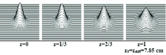
Figure 1: Intensity profiles of a Gaussian beam with initial condition $A_{x}(x,y,z=0)=\exp\left(-\frac{x^{2}+y^{2}}{2}\right)$ governed by the $2D$ paraxial equation (74). The transverse size (the spot) grows by factor $\sqrt{2}$ over normalized distance $z=1$. This correspond to a real distance $z_{0}=z_{diff}^{beam}=7.85$ $cm$ for the selected in the paper laser source on $\lambda_{0}=800$ $nm$.

7 Dynamics of light beam, LF, LB and LD in air

In the beginning of this section we will discuss more widely the Galilean invariancy and connections between normalized equations written in different coordinate systems: Laboratory and Galilean. The Galilean invariancy of the SVEA (45) and VLAE (47) is not obvious. Indeed, after using the transformation $t^{\prime}=t$ and $z^{\prime}=z-vt$ where $v=1$ the new equations in Galilean frame, (46) and (48) admit mixed $z,t$ terms and look quite different. The Galilean invariancy can be seen only from the kind of the fundamental solutions of equations (6)-(6) in Laboratory and Galilean frames. The solutions are equal with precision wave number $k_{z}$, which gives the stationarity in Galilean and translation in z direction in Laboratory frame. The numerical solutions with initial conditions - Gaussian pulses provided in [22] for both coordinate systems demonstrate again that localized waves admit equal spatial and phase deformation in both coordinates and there is only one difference - stationarity in Galilean and translation with normalized velocity v=1 in Laboratory frame. Naturally, the best way is to solve numerically the equations (45) or (47) in Laboratory system and to see one spatial and phase transformation of the pulse as well as its translation. Inconvenience in such one approach is, that at long distances the pulses will move out of the grid. And here the Galilean invariancy of the normalized equations help us. It is well known that the times in Galilean and Laboratory systems are equal $t^{\prime}=t$. As the normalized velocity is $v=1$, the same translation $z=1$ in Laboratory frame correspond to time evolution in both system $t^{\prime}=t=1$ . This is demonstrated in [22] but here it gives us one additional opportunity. We can solve the equation (46) in Galilean frame for long time t’ without pulses to move out of the grid and to connect the normalized time t’ in Galilean with normalized time $t$ and translation $z$ in Laboratory frame $t^{\prime}=t=z;\ v=1$. After that, using normalized constants, we can obtain the real distance of propagation of optical pulses. It is not hard to see that normalized distance $z=1$ correspond to a real distance $z_{0}=k_{0}r_{\perp}^{2}$ when $\alpha\delta^{2}=1$. And this is the natural way to compare the dynamics of optical pulses governed by equation (46) in Galilean frame with the evolution of a laser beam in scalar paraxial approximation described by normalized equation:

$$-i\frac{\partial A}{\partial z}+\frac{1}{2}\Delta_{\bot}A=0,$$ (74)

where, as it is well known, $z=1$ in normalized coordinates corresponds to a real distance $z_{0}=k_{0}r_{\perp}^{2}$ called diffraction length. This length determines the distance where the laser beam increase its width on level $e^{-1}$ from the maximum with factor$\sqrt{2}$. We investigate here only laser sources with spectrally limited, not phase modulated initial Gaussian profile. The optical lens and devices add additional phase modulation on the initial pulse and influenced on the widening in linear regime.

Evolution of real laser pulse with the following characteristics is considered: light source form Ti:sapphire with width on level $e^{-1}$; $r_{\perp}=100$ $\mu m$. Usually such small spot of the pulse is made by focusing by lens. To obtain no modulated in phase initial pulse the additional phase from the lens must be reduced to zero by a system of lens. The solutions of linear SVEA (46) in Galilean frame are carried out for optical wave on wave-length $\lambda_{0}=800$ $nm$ propagating in air and the following constants: carrying wave number $k_{0}=n_{b}\omega/c=7.854\times 10^{4}$; $cm^{-1}$, where $n_{b}\approx 1.0$ for air; GVD coefficient $k"=3.0\times 10^{-31}$ $sec^{2}/cm$; normalized GVD coefficient $\beta_{1}=k_{0}v^{2}k"\cong 2.1\times 10^{-4}$. To find the difference in dynamics of LF, LB, and LD we select different time duration of pulses for LF ($t_{0}=260ps$), LB ($t_{0}=330fs)$ and LD $(t_{0}=33fs$). Using the above parameters of the laser sources and the material constants we obtain the following dimmensionless parameters in SVEA (46) for the particular cases:

a) long pulse and $\alpha\delta^{2}=1$ ($t_{0}=260ps$): $\alpha=6.16\times 10^{5}$; $\delta^{2}=1/6.16\times 10^{-5}$; $\beta_{1}=2.1\times 10^{-4}$.

b) light bullet (330 fs): $\alpha=785.0$; $\delta^{2}=1.0$; $\beta_{1}=2.1\times 10^{-4}$.

c) light disk (33 fs): $\alpha=78,5$; $\delta^{2}=100.0$; $\beta_{1}=2.1\times 10^{-4}$.

Other important parameter for comparing the pulse dynamics and paraxial evolution of a laser beam is the diffraction length $z_{diff}=k_{0}r_{\perp}^{2}=7.85$ $cm$. In addition, we should point out that all coming numerical computations are performed with pulses satisfying the boundary conditions $\lim_{x.y,z\mapsto\pm L/2}A(x,y,z,t)\vec{x}=0$ and also $\lim_{x.y,z\mapsto\pm\Lambda/2}A(k_{x},k_{y},k_{z},t)=0$, where $L$ and $\Lambda$ are respectively the spatial and wave-number intervals for the calculations.

7.1 Evolution of Gaussian beam in paraxial approximation

The initial conditions for linearly polarized normalized Gaussian beam reads:

$$\vec{A}=A_{x}\vec{x};$$

$$A_{x}(x,y,z=0)=\exp\left(-\frac{x^{2}+y^{2}}{2}\right).$$ (75)

The evolution of the initial Gaussian beam (7.1) governed by the paraxial equation (74) is described by the Fresnel’s integral or can be found by numerical calculation of the inverse Fourier transform of the solution in the ($k_{x},k_{y}$)-space. The intensity profile of a solution $A(x,y,z)$ of the paraxial equation (74) with initial condition (7.1) on a normalized distance $z=1$ is illustrated on Fig.1. Getting in ming the above real parameters of a laser system on $800$ $nm$, the normalized distance $z=1$ corresponds to one diffraction length and real distance of $z_{0}=z_{diff}=k_{0}r_{\perp}^{2}=7.85$ $cm$.

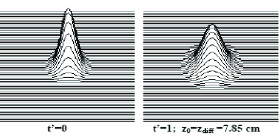
Figure 2: Transverse intensity distribution of $260$ $ps$ pulse on carrying frequency $800$ $nm$ (long Gaussian pulse). Numerical solutions of the linear SVEA (46) in Galilean frame is performed by the following particularly selected initial conditions to satisfy $\alpha\delta^{2}=1$: $A_{x}(x,y,z,t=0)=\exp\left(-\frac{x^{2}+y^{2}+z^{2}}{2}\right)$, $\alpha=6.16\times 10^{5}$; $\delta^{2}=1/6.16\times 10^{-5}$; $\beta_{1}=2.1\times 10^{-4}$. The surfaces $|A(x,y,z^{\prime}=0,t^{\prime}=0;t^{\prime}=1)|^{2}$ are plotted. The transverse size (the spot) grows by factor $\sqrt{2}$ over normalized time-distance $t^{\prime}=z=1$. This correspond to real distance $z_{0}=z_{diff}^{beam}=7.85$ $cm$ equal to the diffraction length of a laser beam (compare with Fig.1).

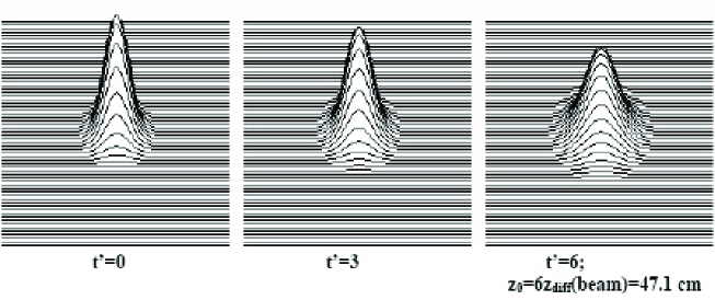
Figure 3: Intensity distribution profiles of $43$ $ps$ pulse on carrying frequency $800$ $nm$ (long Gaussian pulse). Numerical solutions of the linear SVEA (46) in Galilean frame is performed with initial conditions satisfy $\alpha\delta^{2}=6$; $\alpha=1.\times 10^{5}$; $\delta^{2}=6.\times 10^{-5}$; $\beta_{1}=2.1\times 10^{-4}$. The transverse size (the spot) grows by factor $\sqrt{2}$ over normalized time-distance $t^{\prime}=z=6$. This correspond to a real distance $z_{diff}^{pulse}=\alpha\delta^{2}z_{diff}^{beam}=47.1$ $cm$.

7.2 Evolution of long optical pulses (light filaments)

The pointed above choice for the parameter $\alpha\delta^{2}=1$ of a long pulse is used particularly to compare it’s diffraction with the diffraction length of a laser beam. We mark also that in the general case, the real diffraction length of a long pulse (ns or ps) is similar to the diffraction of laser beam and the difference is in the factor $\alpha\delta^{2}$ or:

$$z^{pulse}_{diff}=\alpha\delta^{2}z^{beam}_{diff}=k_{0}^{2}r^{4}_{\perp}/z_{0}.$$ (76)

The validity of this expression is illustrated on the next two figures where the dynamics of an initial long pulse is governed by the linear SVEA (46) in Galilean frame with initial condition $\vec{A}=A_{x}\vec{x};\ A_{x}(x,y,z^{\prime},t^{\prime}=0)=\exp\left(-\frac{x^{2}+y^{2}+z^{\prime 2}}{2}\right)$ and dimensionless constants:

a) long pulse on $260$ $ps$: $\alpha\delta^{2}=1$; $\alpha=6.16\times 10^{5}$; $\delta^{2}=1/6.16\times 10^{-5}$; $\beta_{1}=2.1\times 10^{-4}$.

b) long pulse on $43$ $ps$: $\alpha\delta^{2}=6$; $\alpha=1.\times 10^{-5}$; $\delta^{2}=6.\times 10^{-5}$; $\beta_{1}=2.1\times 10^{-4}$.

Case a) is illustrated on Fig. 2, where the spot (x,y size) of the pulse is plotted and the parameters are selected to satisfy the relation $\alpha\delta^{2}=1$. That is why the pulse enlarge its spatial width by a factor $\sqrt{2}$ on the same normalized time-distance $t^{\prime}=z=1$ as in the case of laser beam. Case b) is illustrated on Fig. 3., where the important dimmensionless parameter is $\alpha\delta^{2}=6$. As can be expected the spot of the pulse grows by factor $\sqrt{2}$ on six time longer distance than a laser beam and the special case a). Summarizing the results obtained for the linear regime of long pulses we conclude: The long optical pulses admit diffraction length of the same order to the one of a laser beam and this length can be equal only in some partial cases, satisfy $\alpha\delta^{2}=1$.

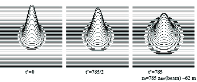
Figure 4: Evolution of a Gaussian light bullet with $330$ $fs$ time duration governed by linear SVEA (46) in Galilean frame under initial condition $A_{x}(x,y,z,t=0)=\exp\left(-\frac{x^{2}+y^{2}+z^{2}}{2}\right)$, $\alpha=785.0;\ \delta=1.0$; $\beta_{1}=2.1\times 10^{-4}$. The surfaces $|A(x,y,z^{\prime}=0;t^{\prime}=0;\ t^{\prime}=785/2;\ t^{\prime}=785)|^{2}$ are plotted. The transverse size (the spot) grows by factor $\sqrt{2}$ over normalized time-distance $t^{\prime}=z=785$. For the selected in the paper laser source this corresponds to a real distance $z_{diff}^{pulse}=\alpha\delta^{2}z_{diff}^{beam}\simeq 62$ $m$.

7.3 Propagation of light bullets in linear regime

The evolution of LB in media with dispersion, is governed by the same SVEA (46) as in the case of long pulses. The shape of the LB is symmetric in the $x$, $y$ and $z$ plane, so that the linearly polarized initial Gaussian profile can be written as:

$$\vec{A}=A_{x}\vec{x};\ \alpha=785;\ \delta^{2}=\frac{r_{\bot^{2}}}{z_{0}^{2}}=1,\ \beta_{1}=2.1\times 10^{-4}$$

$$A_{x}(x,y,z,t=0)=\exp\left(-\frac{x^{2}+y^{2}+z^{2}}{2}\right).$$ (77)

From the qualitative analysis presented in the previous section, when $\delta^{2}=1$, the widening of the LB is expected to be $\alpha=785$; $z^{bullet}_{diff}=\alpha z^{beam}_{diff}=k_{0}^{2}r^{3}_{\perp}$. The surface (x,y plane) of the solution of VLAE (6) with initial conditions of the kind of (7.3) on normalized time-distance $t^{\prime}=z=785$, calculated by exploit of FFT technique, is illustrated on Fig. 4. One can see that the pulse enlarge its spot by factor $\sqrt{2}$ along a considerable distance of $z^{bullet}_{diff}=\alpha z^{beam}_{diff}=785z^{beam}_{diff}=6162.25$ $cm$ $\cong 61$ $m$. Let us remark once again that this result is only correct if the number of harmonics under the pulse, multiplied by $2\pi$ (dimensionless parameter $\alpha$), is large.

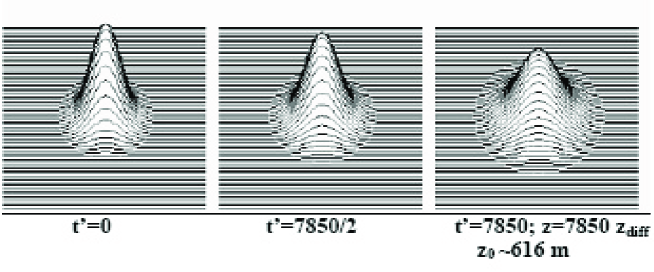
Figure 5: Transverse intensity distribution of $33$ $fs$ pulse on carrying frequency $800$ $nm$ (light disk) governed by the same SVEA (46) and initial condition $A_{x}(x,y,z,t=0)=\exp\left(-\frac{x^{2}+y^{2}+z^{2}}{2}\right)$, $\alpha=78.5;\ \delta=100$; $\beta_{1}=2.1\times 10^{-4}$. The surfaces $|A(x,y,z^{\prime}=0;t^{\prime}=0;\ t^{\prime}=7850/2;\ t^{\prime}=7850)|^{2}$ are presented. The LD enlarges its transverse size by factor $\sqrt{2}$ over the normalized time-distance $t^{\prime}=z=7850$. This correspond to 7850 diffraction lengths of a laser beam or for the selected laser source: $z_{diff}^{pulse}=\alpha\delta^{2}z_{diff}^{beam}\simeq 621$ $m$.

7.4 Dynamics of light disks in linear regime.
Low-diffractive regime

As it was mentioned in the beginning, optical pulses with small longitudinal and large transverse size, while at the same time the large number of harmonics under the pulse remaines, can be obtained without significant experimental difficulties. This can easily be realized in the optical region for pulses with time duration from $200-300$ $fs$ up to $30-40$ $fs$. We consider again the propagation of LD in the framework of the solutions (6) of the SVEA (46) in Galilean coordinates under initial conditions of the form:

$$\vec{A}=A_{x}\vec{x};\ \alpha=78.5;\ \delta^{2}=\frac{r_{\bot^{2}}}{z_{0}^{2}}=100,$$

$$A_{x}(x,y,z^{\prime},t^{\prime}=0)=\exp\left(-\frac{x^{2}+y^{2}+z^{\prime 2}}{2}\right).$$ (78)

Results of calculations of solution (6) with initial conditions of kind (7.4), using FFT and inverse FFT technique are presented on Fig. 5. The numerical solution confirm our expectation that the LD enlarges its shape by factor $\sqrt{2}$ on 7850 time longer distance than the diffraction length of a laser beam; $z^{disk}_{diff}=\alpha\delta^{2}z^{beam}_{diff}=k_{0}^{2}r^{4}_{\perp}/z_{0}=7850z^{beam}_{diff}\cong 616$ $m$. The new formula for diffraction length of optical pulses (76) gives remarkable opportunity to select the parameters of the laser pulse and to obtain pulses with negligible diffraction. From (76) it is seen that $z^{pulse}_{diff}$ depends on the spot diameter of the pulse by four degree ($z^{disk}_{diff}\sim r^{4}_{\perp}$). If we use pulse large enough in transverse dimension we can obtain practically diffractionless pulses. For example, using (76) and light disk with waist $r_{\perp}=1$ $cm$, time duration $t_{0}=33$ $fs$ ($z_{0}=10$ $\mu m$), and $k_{0}=7.85\times 10^{4}$ $cm^{-1}$ ($\lambda_{0}=800$ $nm$) we can obtain pulse diffraction length of order of $z^{disk}_{diff}\sim 6160$ $km$. Such LD will be propagate in transparency region of gases or vacuum on several thousand kilometers without practical diffraction enlargement.

8 Conclusion

In this paper dynamics of ultrashort laser pulses in media with dispersion, dispersionless media and vacuum are investigated in the frame of non-paraxial generalization of the amplitude equation. In partial case of media with dispersion, we obtained an integro - differential nonlinear equation, governing propagation of optical pulses with time duration of order of the optical period. The slowly varying envelope approximation (many harmonics under the pulse) reduced this amplitude integro - differential equation to the well known slowly-varying amplitude vector nonlinear differential equation with different orders of dispersion of the linear and nonlinear susceptibility. In case of propagation of optical pulses in dispersionless media and vacuum, we obtained an nonparaxial amplitude equation which is valid in both cases, namely, pulses with many harmonics and pulses with only one-two harmonics under the envelope. We normalized these amplitude equations and obtained five dimensionless parameters determining different linear and nonlinear regimes. The nonparaxial envelope equations for media with dispersion, dispersionless media and vacuum are solved in linear regime and new fundamental solutions, including the GVD, are found. In gases and vacuum the solutions of these equations predict new diffraction length for optical pulses $z^{pulse}_{diff}=k_{0}^{2}r^{4}_{\perp}/z_{0}$. We demonstrate by these analytical and numerical solutions a significant decreasing of the diffraction enlargement of $fs$ pulses (LB and LD) in respect to paraxial widening of a laser beam and a possibility to reach diffraction-free regime.

9 Acknowledgements

This work is partially supported by the Bulgarian Science Foundation under grant F 1515/2005.

References

- [1] A. Braun, G. Korn, X. Liu, D. Du, J. Squier, and G. Mourou, Self-channeling of high-peak-powerfemtosecond laser pulses in air, Opt. Lett., 20(1), 73-75 (1997).
- [2] C. Ruiz, J. San Romain, C. Mendez, V. Diaz, L. Plaja, I. Arias, and L. Roso, Observation of Spontaneous Self-Chaneling of Light in Air below the Collapse Threshold, Phys. Rev. Lett 95, 053905, (2005).
- [3] J. V. Moloney, M. Kolesik, Full vectorial, intense ultrashort pulse propagators: derivations and applications, Progress in Ultrafast Intense Laser Science II,vol 85, Springer, Berlin.
- [4] A. Couairon, and A. Mysyrowicz, Femtosecond filamentation in transparent media, Physics Reports, 441, 47-189 (2007).
- [5] S. L. Chin, S. A. Hosseini, W. Liu, Q. Luo, F. Théberge, N. Aközbek, A. Becker, V. P. Kandidov, O. G. Kosareva, and H. Schoeder, The propagation of powerful femtosecond laser pulses in optical media: physics, applications, and new challenges Can. J. Phys. 83, 863-905 (2005).
- [6] Y. Silberbers, Collapse of optical pulses, Opt.Lett.,15, 1282-1284(1990).
- [7] P. Chernev and V. Petrov, Self-focusing of light pulses in the presence of normal group velocity dispersion, Opt. Lett. 17, 172-174 (1992).
- [8] I. G. Koprinkov, A. Suda, P. Wang, K. Midorikawa, Self-compression of high intensity femtosecond optical pulses and spatiotemporal solitons, Phys. Rev. Lett. 84(17), 3847-3850(2000).
- [9] Yu. S. Kivshar, G. P. Agrawal, Optical Solitons: From Fibers to Photonic Crystals, Academic Press, Boston, 2003.
- [10] I. P. Christov, Propagation of femtosecond light pulses, 53, 364-366(1985).
- [11] V. I. Karpman, Nonlinear waves in dispersive media, Nauka, Moscow, 1973.
- [12] M. Jain and N. Tzoar, Nonlinear pulse propagation in optical fibres, Opt. Lett 3, 202 (1978).
- [13] J. V. Moloney and A. C. Newell, Nonlinear Optics,Addison-Wesley Publ. Comp.,1991.
- [14] D. N. Christodoulides and R. H. Jouseph, ”Exact radial dependance of the field in a nonlinear dispersive dielectric fiber: bright pulse solutions”. Opt. Lett., 9, 229-231 (1984).
- [15] N. N. Akhmediev and A. Ankiewicz, Solitons: Nonlinear pulses and beams, Chairman and Hall, 1997.
- [16] R. W. Boyd Nonlinear Optics,Academic Press, 2003.
- [17] L. M. Kovachev, Optical Vortices in Dispersive Nonlinear Kerr-type Media, Int. Jour. of Math. and Math. Sci., 18, 949-967(2004).
- [18] G. Fibich, G. S. Papanicolaou, Self-focusing in the presence of small time dispersion and nonparaxiality, Opt. Lett 22, 1379-1381 (1997).
- [19] C. Menyuk, Application of multiple-lenght methods to the study of optical fiber transmision, Journal of Engineering Mathematics, 36, 113-136 (1999).
- [20] T. Brabec, F. Krausz, Nonlinear Optic al Pulse Propagation in Single-Cycle Regime, Phys.Rev. Lett. 78, 3282-3285 (1997).
- [21] K. L. Kovachev, Limits of application of the slowly varying amplitude approximation - Bachelor Thesis, University of Sofia, 2003.
- [22] L. M. Kovachev, L. Pavlov, L. M. Ivanov, and D. Dakova, ”Optical filaments and optical bullets in dispersive nonlinear media”, Journal of Russian Laser Research 27, 185-203(2006).
- [23] L. M. Kovachev, Collapse arrest and self-guiding of femtosecond pulses, Opt. Express, 15, 10318-10323(2007).