Factored Value Iteration Converges

Abstract.

In this paper we propose a novel algorithm, factored value iteration (FVI), for the approximate solution of factored Markov decision processes (fMDPs). The traditional approximate value iteration algorithm is modified in two ways. For one, the least-squares projection operator is modified so that it does not increase max-norm, and thus preserves convergence. The other modification is that we uniformly sample polynomially many samples from the (exponentially large) state space. This way, the complexity of our algorithm becomes polynomial in the size of the fMDP description length. We prove that the algorithm is convergent. We also derive an upper bound on the difference between our approximate solution and the optimal one, and also on the error introduced by sampling. We analyze various projection operators with respect to their computation complexity and their convergence when combined with approximate value iteration.

1. Introduction

Markov decision processes (MDPs) are extremely useful for formalizing and solving sequential decision problems, with a wide repertoire of algorithms to choose from [4, 26]. Unfortunately, MDPs are subject to the ‘curse of dimensionality’ [3]: for a problem with $m$ state variables, the size of the MDP grows exponentially with $m$, even though many practical problems have polynomial-size descriptions. Factored MDPs (fMDPs) may rescue us from this explosion, because they offer a more compact representation [17, 5, 6]. In the fMDP framework, one assumes that dependencies can be factored to several easy-to-handle components.

For MDPs with known parameters, there are three basic solution methods (and, naturally, countless variants of them): value iteration, policy iteration and linear programming (see the books of Sutton & Barto [26] or Bertsekas & Tsitsiklis [4] for an excellent overview). Out of these methods, linear programming is generally considered less effective than the others. So, it comes as a surprise that all effective fMDPs algorithms, to our best knowledge, use linear programming in one way or another. Furthermore, the classic value iteration algorithm is known to be divergent when function approximation is used [2, 27], which includes the case of fMDPs, too.

In this paper we propose a variant of the approximate value iteration algorithm for solving fMDPs. The algorithm is a direct extension of the traditional value iteration algorithm. Furthermore, it avoids computationally expensive manipulations like linear programming or the construction of decision trees. We prove that the algorithm always converges to a fixed point, and that it requires polynomial time to reach a fixed accuracy. A bound to the distance from the optimal solution is also given.

In Section 2 we review the basic concepts of Markov decision processes, including the classical value iteration algorithm and its combination with linear function approximation. We also give a sufficient condition for the convergence of approximate value iteration, and list several examples of interest. In Section 3 we extend the results of the previous section to fMDPs and review related works in Section 4. Conclusions are drawn in Section 5.

2. Approximate Value Iteration in Markov Decision Processes

2.1. Markov Decision Processes

An MDP is characterized by a sixtuple $(\mathbf{X},A,R,P,\mathbf{x}_{s},\gamma)$, where $\mathbf{X}$ is a finite set of states; $A$ is a finite set of possible actions; $R:\mathbf{X}\times A\to\mathbb{R}$ is the reward function of the agent, so that $R(\mathbf{x},a)$ is the reward of the agent after choosing action $a$ in state $\mathbf{x}$; $P:\mathbf{X}\times A\times\mathbf{X}\to[0,1]$ is the transition function so that $P(\mathbf{y}\mid\mathbf{x},a)$ is the probability that the agent arrives at state $\mathbf{y}$, given that she started from $\mathbf{x}$ upon executing action $a$; $\mathbf{x}_{s}\in\mathbf{X}$ is the starting state of the agent; and finally, $\gamma\in[0,1)$ is the discount rate on future rewards.

A policy of the agent is a mapping $\pi:\mathbf{X}\times A\to[0,1]$ so that $\pi(\mathbf{x},a)$ tells the probability that the agent chooses action $a$ in state $\mathbf{x}$. For any $\mathbf{x}_{0}\in\mathbf{X}$, the policy of the agent and the parameters of the MDP determine a stochastic process experienced by the agent through the instantiation

$$\mathbf{x}_{0},a_{0},r_{0},\mathbf{x}_{1},a_{1},r_{1},\ldots,\mathbf{x}_{t},a_{t},r_{t},\ldots$$

The goal is to find a policy that maximizes the expected value of the discounted total reward. Let the value function of policy $\pi$ be

$$V^{\pi}(\mathbf{x}):=E\Bigl{(}\sum_{t=0}^{\infty}\gamma^{t}r_{t}\Bigm{|}\mathbf{x}\!=\!\mathbf{x}_{0}\Bigr{)}$$

and let the optimal value function be

$$V^{*}(\mathbf{x}):=\max_{\pi}V^{\pi}(\mathbf{x})$$

for each $\mathbf{x}\in\mathbf{X}$. If $V^{*}$ is known, it is easy to find an optimal policy $\pi^{*}$, for which $V^{\pi^{*}}\equiv V^{*}$. Provided that history does not modify transition probability distribution $P(\mathbf{y}|\mathbf{x},a)$ at any time instant, value functions satisfy the famous Bellman equations

(1) $$V^{\pi}(\mathbf{x})=\sum_{a}\sum_{\mathbf{y}}\pi(\mathbf{x},a)P(\mathbf{y}\mid\mathbf{x},a)\Bigl{(}R(\mathbf{x},a)+\gamma V^{\pi}(\mathbf{y})\Bigr{)}$$

and

(2) $$V^{*}(\mathbf{x})=\max_{a}\sum_{\mathbf{y}}P(\mathbf{y}\mid\mathbf{x},a)\Bigl{(}R(\mathbf{x},a)+\gamma V^{*}(\mathbf{y})\Bigr{)}.$$

Most algorithms that solve MDPs build upon some version of the Bellman equations. In the following, we shall concentrate on the value iteration algorithm.

2.2. Exact Value Iteration

Consider an MDP $(\mathbf{X},A,P,R,\mathbf{x}_{s},\gamma)$. The value iteration for MDPs uses the Bellman equations (2) as an iterative assignment: It starts with an arbitrary value function $V_{0}:\mathbf{X}\to\mathbb{R}$, and in iteration $t$ it performs the update

(3) $$V_{t+1}(\mathbf{x}):=\max_{a}\sum_{\mathbf{y}\in\mathbf{X}}P(\mathbf{y}\mid\mathbf{x},a)\Bigl{(}R(\mathbf{x},a)+\gamma V_{t}(\mathbf{y})\Bigr{)}$$

for all $\mathbf{x}\in\mathbf{X}$. For the sake of better readability, we shall introduce vector notation. Let $N:=|\mathbf{X}|$, and suppose that states are integers from 1 to $N$, i.e. $\mathbf{X}=\{1,2,\ldots,N\}$. Clearly, value functions are equivalent to $N$-dimensional vectors of reals, which may be indexed with states. The vector corresponding to $V$ will be denoted as $\mathbf{v}$ and the value of state $\mathbf{x}$ by ${\mathbf{v}}_{\mathbf{x}}$. Similarly, for each $a$ let us define the $N$-dimensional column vector $\mathbf{r}^{a}$ with entries $\mathbf{r}^{a}_{\mathbf{x}}=R(\mathbf{x},a)$ and $N\times N$ matrix $P^{a}$ with entries $P^{a}_{\mathbf{x},\mathbf{y}}=P(\mathbf{y}\mid\mathbf{x},a)$. With these notations, (3) can be written compactly as

(4) $$\mathbf{v}_{t+1}:=\textbf{max}_{a\in A}\bigl{(}\mathbf{r}^{a}+\gamma P^{a}\mathbf{v}_{t}\bigr{)}.$$

Here, max denotes the componentwise maximum operator.

It is also convenient to introduce the Bellman operator $\mathcal{T}:\mathbb{R}^{N}\to\mathbb{R}^{N}$ that maps value functions to value functions as

$$\mathcal{T}\mathbf{v}:=\textbf{max}_{a\in A}\bigl{(}\mathbf{r}^{a}+\gamma P^{a}\mathbf{v}\bigr{)}.$$

As it is well known, $\mathcal{T}$ is a max-norm contraction with contraction factor $\gamma$: for any $\mathbf{v},\mathbf{u}\in\mathbb{R}^{N}$, $\|\mathcal{T}\mathbf{v}-\mathcal{T}\mathbf{u}\|_{\infty}\leq\gamma\|\mathbf{v}-\mathbf{u}\|_{\infty}$. Consequently, by Banach’s fixed point theorem, exact value iteration (which can be expressed compactly as $\mathbf{v}_{t+1}:=\mathcal{T}\mathbf{v}_{t}$) converges to an unique solution $\mathbf{v}^{*}$ from any initial vector $\mathbf{v}_{0}$, and the solution $\mathbf{v}^{*}$ satisfies the Bellman equations (2). Furthermore, for any required precision $\epsilon>0$, $\|\mathbf{v}_{t}-\mathbf{v}^{*}\|_{\infty}\leq\epsilon$ if $t\geq\frac{\log\epsilon}{\log\gamma}\|\mathbf{v}_{0}-\mathbf{v}^{*}\|_{\infty}$. One iteration costs $O(N^{2}\cdot|A|)$ computation steps.

2.3. Approximate value iteration

In this section we shall review approximate value iteration (AVI) with linear function approximation (LFA) in ordinary MDPs. The results of this section hold for AVI in general, but if we can perform all operations effectively on compact representations (i.e. execution time is polynomially bounded in the number of variables instead of the number of states), then the method can be directly applied to the domain of factorized Markovian decision problems, underlining the importance of our following considerations.

Suppose that we wish to express the value functions as the linear combination of $K$ basis functions $h_{k}:\mathbf{X}\to\mathbb{R}\ \ (k\in\{1,\ldots,K\})$, where $K<<N$. Let $H$ be the $N\times K$ matrix with entries $H_{\mathbf{x},k}=h_{k}(\mathbf{x})$. Let $\mathbf{w}_{t}\in\mathbb{R}^{K}$ denote the weight vector of the basis functions at step $t$. We can substitute $\mathbf{v}_{t}=H\mathbf{w}_{t}$ into the right hand side (r.h.s.) of (4), but we cannot do the same on the left hand side (l.h.s.) of the assignment: in general, the r.h.s. is not contained in the image space of $H$, so there is no such $\mathbf{w}_{t+1}$ that

$$H\mathbf{w}_{t+1}=\textbf{max}_{a\in A}\bigl{(}\mathbf{r}^{a}+\gamma P^{a}H\mathbf{w}_{t}\bigr{)}.$$

We can put the iteration into work by projecting the right-hand side into $\mathbf{w}$-space: let $\mathcal{G}:\mathbb{R}^{N}\to\mathbb{R}^{K}$ be a (possibly non-linear) mapping, and consider the iteration

(5) $$\mathbf{w}_{t+1}:=\mathcal{G}\bigl{[}\textbf{max}_{a\in A}\bigl{(}\mathbf{r}^{a}+\gamma P^{a}H\mathbf{w}_{t}\bigr{)}\bigr{]}$$

with an arbitrary starting vector $\mathbf{w}_{0}$.

Lemma 2.1.

If $\mathcal{G}$ is such that $H\mathcal{G}$ is a non-expansion, i.e., for any $\mathbf{v},\mathbf{v}^{\prime}\in\mathbb{R}^{N}$,

$$\|H\mathcal{G}\mathbf{v}-H\mathcal{G}\mathbf{v}^{\prime}\|_{\infty}\leq\|\mathbf{v}-\mathbf{v}^{\prime}\|_{\infty},$$

then there exists a $\mathbf{w}^{*}\in\mathbb{R}^{K}$ such that

$$\mathbf{w}^{*}=\mathcal{G}\bigl{[}\emph{{max}}_{a\in A}\bigl{(}\mathbf{r}^{a}+\gamma P^{a}H\mathbf{w}^{*}\bigr{)}\bigr{]}$$

and iteration (5) converges to $\mathbf{w}^{*}$ from any starting point.

Proof.

We can write (5) compactly as $\mathbf{w}_{t+1}=\mathcal{G}\mathcal{T}H\mathbf{w}_{t}$. Let $\widehat{\mathbf{v}}_{t}=H\mathbf{w}_{t}$. This satisfies

(6) $$\widehat{\mathbf{v}}_{t+1}=H\mathcal{G}\mathcal{T}\widehat{\mathbf{v}}_{t}.$$

It is easy to see that the operator $H\mathcal{G}\mathcal{T}$ is a contraction: for any $\mathbf{v},\mathbf{v}^{\prime}\in\mathbb{R}^{N}$,

$$\|H\mathcal{G}\mathcal{T}\mathbf{v}-H\mathcal{G}\mathcal{T}\mathbf{v}^{\prime}\|_{\infty} \leq \|\mathcal{T}\mathbf{v}-\mathcal{T}\mathbf{v}^{\prime}\|_{\infty}\leq\gamma\|\mathbf{v}-\mathbf{v}^{\prime}\|_{\infty}$$

by the assumption of the lemma and the contractivity of $\mathcal{T}$. Therefore, by Banach’s fixed point theorem, there exists a vector $\widehat{\mathbf{v}}^{*}\in\mathbb{R}^{N}$ such that $\widehat{\mathbf{v}}^{*}=H\mathcal{G}\mathcal{T}\widehat{\mathbf{v}}^{*}$ and iteration (6) converges to $\widehat{\mathbf{v}}^{*}$ from any starting point. It is easy to see that $\mathbf{w}^{*}=\mathcal{G}T\widehat{\mathbf{v}}^{*}$ satisfies the statement of the lemma.

∎

Note that if $\mathcal{G}$ is a linear mapping with matrix $G\in\mathbb{R}^{K\times N}$, then the assumption of the lemma is equivalent to $\|HG\|_{\infty}\leq 1$.

2.4. Examples of Projections, Convergent and Divergent

In this section, we examine certain possibilities for choosing projection $\mathcal{G}$. Let $\mathbf{v}\in\mathbb{R}^{N}$ be an arbitrary vector, and let $\mathbf{w}=\mathcal{G}\mathbf{v}$ be its $\mathcal{G}$-projection. For linear operators, $\mathcal{G}$ can be represented in matrix form and we shall denote it by $G$.

Least-squares ($L_{2}$-)projection. Least-squares fitting is used almost exclusively for projecting value functions, and the term AVI is usually used in the sense “AVI with least-squares projection”. In this case, $\mathbf{w}$ is chosen so that it minimizes the least-squares error:

$$\mathbf{w}:=\arg\min_{\mathbf{w}}\|H\mathbf{w}-\mathbf{v}\|^{2}_{2}.$$

This corresponds to the linear projection $G_{2}=H^{+}$ (i.e., $\mathbf{w}=H^{+}\mathbf{v}$), where $H^{+}$ is the Moore-Penrose pseudoinverse of $H$. It is well known, however, that this method can diverge. For an example on such divergence, see, e.g. the book of Bertsekas & Tsitsiklis [4]. The reason is simple: matrix $HH^{+}$ is a non-expansion in $L_{2}$-norm, but Lemma 1 requires that it should be an $L_{\infty}$-norm projection, which does not hold in the general case. (See also Appendix A.1 for illustration.)

Constrained least-squares projection. One can enforce the non-expansion property by expressing it as a constraint: Let $\mathbf{w}$ be the solution of the constrained minimization problem

$$\mathbf{w}:=\arg\min_{\mathbf{w}}\|H\mathbf{w}-\mathbf{v}\|^{2}_{2},\textrm{ subject to }\|H\mathbf{w}\|_{\infty}\leq\|\mathbf{v}\|_{\infty},$$

which defines a non-linear mapping $\mathcal{G}_{2}^{c}$. This projection is computationally highly demanding: in each step of the iteration, one has to solve a quadratic programming problem.

Max-norm ($L_{\infty}$-)projection. Similarly to $L_{2}$-projection, we can also select $\mathbf{w}$ so that it minimizes the max-norm of the residual:

$$\mathbf{w}:=\arg\min_{\mathbf{w}}\|H\mathbf{w}-\mathbf{v}\|_{\infty}.$$

The computation of $\mathbf{w}$ can be transcribed into a linear programming task and that defines the non-linear mapping $\mathcal{G}_{\infty}$. However, in general, $\|H\mathcal{G}_{\infty}\mathbf{v}\|_{\infty}\nleq\|\mathbf{v}\|_{\infty}$, and consequently AVI using iteration

$$\mathbf{w}_{t+1}:=\arg\min_{\mathbf{w}}\|H\mathbf{w}-\mathcal{T}H\mathbf{w}_{t}\|_{\infty}$$

can be divergent. Similarly to $L_{2}$ projection, one can also introduce a constrained version $\mathcal{G}_{\infty}^{c}$ defined by

$$\mathcal{G}_{\infty}^{c}\mathbf{v}:=\arg\min_{\mathbf{w}}\|H\mathbf{w}-\mathbf{v}\|_{\infty},\textrm{ subject to }\|H\mathbf{w}\|_{\infty}\leq\|\mathbf{v}\|_{\infty},$$

which can also be turned into a linear program.

It is insightful to contrast this with the approximate linear programming method of Guestrin et al. [13]: they directly minimize the max-norm of the Bellman error, i.e., they solve the problem

$$\mathbf{w}^{*}:=\arg\min_{\mathbf{w}}\|H\mathbf{w}-\mathcal{T}H\mathbf{w}\|_{\infty},$$

which can be solved without constraints.

$L_{1}$-norm projection. Let $\mathcal{G}_{L_{1}}$ be defined by

$$\mathcal{G}_{1}\mathbf{v}:=\arg\min_{\mathbf{w}}\|H\mathbf{w}-\mathbf{v}\|_{1}.$$

The $L_{1}$-norm projection also requires the solution of a linear program, but interestingly, the projection operator $\mathcal{G}_{1}$ is a non-expansion (the proof can be found in Appendix A.1).

AVI-compatible operators considered so far ($\mathcal{G}_{2}^{c}$, $\mathcal{G}_{\infty}^{c}$ and $\mathcal{G}_{1}$) were non-linear, and required the solution of a linear program or a quadratic program in each step of value iteration, which is clearly cumbersome. On the other hand, while $G_{2}\mathbf{v}=H^{+}\mathbf{v}$ is linear, it is also known to be incompatible with AVI [2, 27]. Now, we shall focus on operators that are both AVI-compatible and linear.

Normalized linear mapping. Let $G$ be an arbitrary $K\times N$ matrix, and define its normalization $\mathcal{N}(G)$ as a matrix with the same dimensions and entries

$$[\mathcal{N}(G)]_{i,j}:=\frac{G_{i,j}}{\bigl{(}\sum_{j^{\prime}}|H_{i,j^{\prime}}|\bigr{)}\bigl{(}\sum_{i^{\prime}}|G_{i^{\prime},j}|\bigr{)}},$$

that is, $N(G)$ is obtained from $G$ by dividing each element with the corresponding row sum of $H$ and the corresponding column sum of $G$. All (absolute) row sums of $H\cdot\mathcal{N}(G)$ are equal to 1. Therefore, (i) $\|H\cdot\mathcal{N}(G)\|_{\infty}=1$, and (ii) $H\cdot N(G)$ is maximal in the sense that if the absolute value of any element of $\mathcal{N}(G)$ increased, then for the resulting matrix $G^{\prime}$, $\|H\cdot G^{\prime}\|_{\infty}>1$.

Probabilistic linear mapping. If all elements of $H$ are nonnegative and all the row-sums of $H$ are equal, then $\mathcal{N}(H^{T})$ assumes a probabilistic interpretation. This interpretation is detailed in Appendix A.2.

Normalized least-squares projection. Among all linear operators, $H^{+}$ is the one that guarantees the best least-squares error, therefore we may expect that its normalization, $\mathcal{N}(H^{+})$ plays a similar role among AVI-compatible linear projections. Unless noted otherwise, we will use the projection $\mathcal{N}(H^{+})$ subsequently.

2.5. Convergence properties

Lemma 2.2.

Let $\mathbf{v}^{*}$ be the optimal value function and $\mathbf{w}^{*}$ be the fixed point of the approximate value iteration (5). Then

$$\|H\mathbf{w}^{*}-\mathbf{v}^{*}\|_{\infty}\leq\frac{1}{1-\gamma}\|H\mathcal{G}\mathbf{v}^{*}-\mathbf{v}^{*}\|_{\infty}.$$

Proof.

For the optimal value function, $\mathbf{v}^{*}=\mathcal{T}\mathbf{v}^{*}$ holds. On the other hand, $\mathbf{w}^{*}=\mathcal{G}\mathcal{T}H\mathbf{w}^{*}$. Thus,

$$\|H\mathbf{w}^{*}-\mathbf{v}^{*}\|_{\infty} = \|H\mathcal{G}\mathcal{T}H\mathbf{w}^{*}-\mathcal{T}\mathbf{v}^{*}\|_{\infty}$$

$$\leq \|H\mathcal{G}\mathcal{T}H\mathbf{w}^{*}-H\mathcal{G}\mathcal{T}\mathbf{v}^{*}\|_{\infty}+\|H\mathcal{G}\mathcal{T}\mathbf{v}^{*}-\mathcal{T}\mathbf{v}^{*}\|_{\infty}$$

$$\leq \|\mathcal{T}H\mathbf{w}^{*}-\mathcal{T}\mathbf{v}^{*}\|_{\infty}+\|H\mathcal{G}\mathbf{v}^{*}-\mathbf{v}^{*}\|_{\infty}$$

$$\leq \gamma\|H\mathbf{w}^{*}-\mathbf{v}^{*}\|_{\infty}+\|H\mathcal{G}\mathbf{v}^{*}-\mathbf{v}^{*}\|_{\infty},$$

from which the statement of the lemma follows. For the transformations we have applied the triangle inequality, the non-expansion property of $H\mathcal{G}$ and the contraction property of $\mathcal{T}$. ∎

According to the lemma, the error bound is proportional to the projection error of $\mathbf{v}^{*}$. Therefore, if $\mathbf{v}^{*}$ can be represented in the space of basis functions with small error, then our AVI algorithm gets close to the optimum. Furthermore, the lemma can be used to check a posteriori how good our basis functions are. One may improve the set of basis functions iteratively. Similar arguments have been brought up by Guestrin et al. [13], in association with their LP-based solution algorithm.

3. Factored value iteration

MDPs are attractive because solution time is polynomial in the number of states. Consider, however, a sequential decision problem with $m$ variables. In general, we need an exponentially large state space to model it as an MDP. So, the number of states is exponential in the size of the description of the task. Factored Markov decision processes may avoid this trap because of their more compact task representation.

3.1. Factored Markov decision processes

We assume that $\mathbf{X}$ is the Cartesian product of $m$ smaller state spaces (corresponding to individual variables):

$$\mathbf{X}=X_{1}\times X_{2}\times\ldots\times X_{m}.$$

For the sake of notational convenience we will assume that each $X_{i}$ has the same size, $|X_{1}|=|X_{2}|=\ldots=|X_{m}|=n$. With this notation, the size of the full state space is $N=|\mathbf{X}|=n^{m}$. We note that all derivations and proofs carry through to different size variable spaces.

A naive, tabular representation of the transition probabilities would require exponentially large space (that is, exponential in the number of variables $m$). However, the next-step value of a state variable often depends only on a few other variables, so the full transition probability can be obtained as the product of several simpler factors. For a formal description, we introduce several notations:

For any subset of variable indices $Z\subseteq\{1,2,\ldots,m\}$, let $\mathbf{X}[Z]:=\mathop{\times}\limits_{i\in Z}X_{i}$, furthermore, for any $\mathbf{x}\in\mathbf{X}$, let $\mathbf{x}[Z]$ denote the value of the variables with indices in $Z$. We shall also use the notation $\mathbf{x}[Z]$ without specifying a full vector of values $\mathbf{x}$, in such cases $\mathbf{x}[Z]$ denotes an element in $\mathbf{X}[Z]$. For single-element sets $Z=\{i\}$ we shall also use the shorthand $\mathbf{x}[\{i\}]=\mathbf{x}[i]$.

A function $f$ is a local-scope function if it is defined over a subspace $\mathbf{X}[Z]$ of the state space, where $Z$ is a (presumably small) index set. The local-scope function $f$ can be extended trivially to the whole state space by $f(\mathbf{x}):=f(\mathbf{x}[Z])$. If $|Z|$ is small, local-scope functions can be represented efficiently, as they can take only $n^{|Z|}$ different values.

Suppose that for each variable $i$ there exist neighborhood sets $\Gamma_{i}$ such that the value of $\mathbf{x}_{t+1}[i]$ depends only on $\mathbf{x}_{t}[\Gamma_{i}]$ and the action $a_{t}$ taken. Then we can write the transition probabilities in a factored form

(7) $$P(\mathbf{y}\mid\mathbf{x},a)=\prod_{i=1}^{n}P_{i}(\mathbf{y}[i]\mid\mathbf{x}[\Gamma_{i}],a)$$

for each $\mathbf{x},\mathbf{y}\in\mathbf{X}$, $a\in A$, where each factor is a local-scope function

(8) $$P_{i}:\mathbf{X}[\Gamma_{i}]\times A\times X_{i}\to[0,1]\qquad\textrm{(for all $i\in\{1,\ldots,m\}$).}$$

We will also suppose that the reward function is the sum of $J$ local-scope functions:

(9) $$R(\mathbf{x},a)=\sum_{j=1}^{J}R_{j}(\mathbf{x}[Z_{j}],a),$$

with arbitrary (but preferably small) index sets $Z_{j}$, and local-scope functions

(10) $$R_{j}:\mathbf{X}[Z_{j}]\times A\to\mathbb{R}\qquad\textrm{(for all $j\in\{1,\ldots,J\}$).}$$

To sum up, a factored Markov decision process is characterized by the parameters $\Bigl{(}\{X_{i}:1\leq i\leq m\};A;\{R_{j}:1\leq j\leq J\};\{\Gamma_{i}:1\leq i\leq n\};\{P_{i}:1\leq i\leq n\};\mathbf{x}_{s};\gamma\Bigr{)},$ where $\mathbf{x}_{s}$ denotes the initial state.

Functions $P_{i}$ and $R_{i}$ are usually represented either as tables or dynamic Bayesian networks. If the maximum size of the appearing local scopes is bounded by some constant, then the description length of an fMDP is polynomial in the number of variables $n$.

3.1.1. Value functions

The optimal value function is an $N=n^{m}$-dimensional vector. To represent it efficiently, we should rewrite it as the sum of local-scope functions with small domains. Unfortunately, in the general case, no such factored form exists [13].

However, we can still approximate $V^{*}$ with such an expression: let $K$ be the desired number of basis functions and for each $k\in\{1,\ldots,K\}$, let $C_{k}$ be the domain set of the local-scope basis function $h_{k}:\mathbf{X}[C_{k}]\to\mathbb{R}$. We are looking for a value function of the form

(11) $$\tilde{V}(\mathbf{x})=\sum_{k=1}^{K}w_{k}\cdot h_{k}(\mathbf{x}[C_{k}]).$$

The quality of the approximation depends on two factors: the choice of the basis functions and the approximation algorithm. Basis functions are usually selected by the experiment designer, and there are no general guidelines how to automate this process. For given basis functions, we can apply a number of algorithms to determine the weights $w_{k}$. We give a short overview of these methods in Section 4. Here, we concentrate on value iteration.

3.2. Exploiting factored structure in value iteration

For fMDPs, we can substitute the factored form of the transition probabilities (7), rewards (9) and the factored approximation of the value function (11) into the AVI formula (5), which yields

$$\sum_{k=1}^{K}h_{k}(\mathbf{x}[C_{k}])\cdot w_{k,t+1} \approx \max_{a}\sum_{\mathbf{y}\in\mathbf{X}}\Bigl{(}\prod_{i=1}^{m}P_{i}(\mathbf{y}[i]\mid\mathbf{x}[\Gamma_{i}],a)\Bigr{)}\cdot$$

$$\cdot\Bigl{(}\sum_{j=1}^{J}R_{j}(\mathbf{x}[Z_{j}],a)+\gamma\sum_{k^{\prime}=1}^{K}h_{k^{\prime}}(\mathbf{y}[C_{k^{\prime}}])\cdot w_{k^{\prime},t}\Bigr{)}.$$

By rearranging operations and exploiting that all occurring functions have a local scope, we get

$$\sum_{k=1}^{K}h_{k}(\mathbf{x}[C_{k}])\cdot w_{k,t+1}=\mathcal{G}_{k}\max_{a}\Biggl{[}\sum_{j=1}^{J}R_{j}(\mathbf{x}[Z_{j}],a)$$

(12) $$+\gamma\sum_{k^{\prime}=1}^{K}\sum_{\mathbf{y}[C_{k^{\prime}}]\in\mathbf{X}[C_{k^{\prime}}]}\Bigl{(}\prod_{i\in C_{k^{\prime}}}P_{i}(\mathbf{y}[i]\mid\mathbf{x}[\Gamma_{i}],a)\Bigr{)}h_{k^{\prime}}(\mathbf{y}[C_{k^{\prime}}])\cdot w_{k^{\prime},t}\Biggr{]}$$

for all $\mathbf{x}\in\mathbf{X}$. We can write this update rule more compactly in vector notation. Let

$$\mathbf{w}_{t}:=(w_{1,t},w_{2,t},\ldots,w_{K,t})\in\mathbb{R}^{K},$$

and let $H$ be an $|\mathbf{X}|\times K$ matrix containing the values of the basis functions. We index the rows of matrix $H$ by the elements of $\mathbf{X}$:

$$H_{\mathbf{x},k}:=h_{k}(\mathbf{x}[C_{k}]).$$

Further, for each $a\in A$, let $B^{a}$ be the $|\mathbf{X}|\times K$ value backprojection matrix defined as

$$B^{a}_{\mathbf{x},k}:=\sum_{\mathbf{y}[C_{k}]\in\mathbf{X}[C_{k}]}\Bigl{(}\prod_{i\in C_{k}}P_{i}(\mathbf{y}[i]\mid\mathbf{x}[\Gamma_{i}],a)\Bigr{)}h_{k}(\mathbf{y}[C_{k}])$$

and for each $a$, define the reward vector $\mathbf{r}^{a}\in\mathbb{R}^{|\mathbf{X}|}$ by

$$\mathbf{r}^{a}_{\mathbf{x}}:=\sum_{j=1}^{n_{r}}R_{j}(\mathbf{x}[Z_{j}],a).$$

Using these notations, (12) can be rewritten as

(13) $$\mathbf{w}_{t+1}:=\mathcal{G}\textbf{max}_{a\in A}\Bigl{(}\mathbf{r}^{a}+\gamma B^{a}\mathbf{w}_{t}\Bigr{)}.$$

Now, all entries of $B^{a}$, $H$ and $\mathbf{r}^{a}$ are composed of local-scope functions, so any of their individual elements can be computed efficiently. This means that the time required for the computation is exponential in the sizes of function scopes, but only polynomial in the number of variables, making the approach attractive. Unfortunately, the matrices are still exponentially large, as there are exponentially many equations in (12). One can overcome this problem by sampling as we show below.

3.3. Sampling

To circumvent the problem of having exponentially many equations, we select a random subset $\widehat{\mathbf{X}}\subseteq\mathbf{X}$ of the original state space so that $|\widehat{\mathbf{X}}|=\textrm{poly}(m)$, consequently, solution time will scale polynomially with $m$. On the other hand, we will select a sufficiently large subset so that the remaining system of equations is still over-determined. The necessary size of the selected subset is to be determined later: it should be as small as possible, but the solution of the reduced equation system should remain close to the original solution with high probability. For the sake of simplicity, we assume that the projection operator $\mathcal{G}$ is linear with matrix $G$. Let the sub-matrices of $G$, $H$, $B^{a}$ and $\mathbf{r}^{a}$ corresponding to $\widehat{\mathbf{X}}$ be denoted by $\widehat{G}$, $\widehat{H}$, $\widehat{B}^{a}$ and $\widehat{\mathbf{r}}^{a}$, respectively. Then the following value update

(14) $$\mathbf{w}_{t+1}:=\widehat{G}\cdot\textbf{max}_{a\in A}\Bigl{(}\widehat{\mathbf{r}}^{a}+\gamma\widehat{B}^{a}\mathbf{w}_{t}\Bigr{)}$$

can be performed effectively, because these matrices have polynomial size. Now we show that the solution from sampled data is close to the true solution with high probability.

Theorem 3.1.

Let $\mathbf{w}^{*}$ be the unique solution of $\mathbf{w}^{*}=G\mathcal{T}H\mathbf{w}^{*}$ of an FMDP, and let ${\mathbf{w}}^{\prime}$ be the solution of the corresponding equation with sampled matrices, ${\mathbf{w}}^{\prime}=\widehat{G}\mathcal{T}\widehat{H}{\mathbf{w}}^{\prime}$. Suppose that the projection matrix $G$ has a factored structure, too. Then iteration (14) converges to $\mathbf{w}^{\prime}$, furthermore, for a suitable constant $\,\Xi$ (depending polynomially on $n^{z}$, where $z$ is the maximum cluster size), and for any $\epsilon,\delta>0$, $\|\mathbf{w}^{*}-\mathbf{w}^{\prime}\|_{\infty}\leq\epsilon$ holds with probability at least $1-\delta$, if the sample size satisfies $\displaystyle N_{1}\geq\Xi\frac{m^{2}}{\epsilon^{2}}\log\frac{m}{\delta}$.

The proof of Theorem 3.1 can be found in Appendix A.3. The derivation is closely related to the work of Drineas and colleagues [11, 12], although we use the infinity-norm instead of the $L_{2}$-norm. A more important difference is that we can exploit the factored structure, gaining an exponentially better bound. The resulting factored value iteration algorithm is summarized in Table 1.

Algorithm 1 Factored value iteration with a linear projection matrix $G$.

  % inputs:

  % factored MDP, $\mathcal{M}=\bigl{(}\{X_{i}\}_{i=1}^{m};A;\{R_{j}\}_{j=1}^{J};\{\Gamma_{i}\}_{i=1}^{m};\{P_{i}\}_{i=1}^{m};\mathbf{x}_{s};\gamma\bigr{)}$

  % basis functions, $\{h_{k}\}_{k=1}^{K}$

  % required accuracy, $\epsilon$

  $N_{0}:=$ number of samples

  $\widehat{\mathbf{X}}:=$ uniform random $N_{0}$-element subset of $\mathbf{X}$

  create $\widehat{H}$ and $\widehat{G}$

  create $\widehat{B}^{a}=\widehat{P^{a}H}$ and $\widehat{\mathbf{r}}^{a}$ for each $a\in A$

  $\mathbf{w}_{0}=\mathbf{0}$, $t:=0$

  repeat

     $\displaystyle\mathbf{w}_{t+1}:=\widehat{G}\cdot\max_{a\in A}\Bigl{(}\widehat{\mathbf{r}}^{a}+\gamma\widehat{B}^{a}\mathbf{w}_{t}\Bigr{)}$

     $\Delta_{t}:=\|\mathbf{w}_{t+1}-\mathbf{w}_{t}\|_{\infty}$

     $t:=t+1$

  until $\Delta_{t}\geq\epsilon$

  return  $\mathbf{w}_{t}$

4. Related work

The exact solution of factored MDPs is infeasible. The idea of representing a large MDP using a factored model was first proposed by Koller & Parr [17] but similar ideas appear already in the works of Boutilier, Dearden, & Goldszmidt [5, 6]. More recently, the framework (and some of the algorithms) was extended to fMDPs with hybrid continuous-discrete variables [18] and factored partially observable MDPs [23]. Furthermore, the framework has also been applied to structured MDPs with alternative representations, e.g., relational MDPs [15] and first-order MDPs [24].

4.1. Algorithms for solving factored MDPs

There are two major branches of algorithms for solving fMDPs: the first one approximates the value functions as decision trees, the other one makes use of linear programming.

Decision trees (or equivalently, decision lists) provide a way to represent the agent’s policy compactly. Koller & Parr [17] and Boutilier et al. [5, 6] present algorithms to evaluate and improve such policies, according to the policy iteration scheme. Unfortunately, the size of the policies may grow exponentially even with a decision tree representation [6, 20].

The exact Bellman equations (2) can be transformed to an equivalent linear program with $N$ variables $\{V(\mathbf{x}):\mathbf{x}\in\mathbf{X}\}$ and $N\cdot|A|$ constraints:

maximize: $$\sum_{\mathbf{x}\in\mathbf{X}}\alpha(\mathbf{x})V(\mathbf{x})$$

subject to $$V(\mathbf{x})\leq R(\mathbf{x},a)+\gamma\sum_{\mathbf{x}^{\prime}\in\mathbf{X}}P(\mathbf{x}^{\prime}\mid\mathbf{x},a)V(\mathbf{x}^{\prime}),\quad\textrm{$(\forall\mathbf{x}\in\mathbf{X},a\in A)$.}$$

Here, weights $\alpha(\mathbf{x})$ are free parameters and can be chosen freely in the following sense: the optimum solution is $V^{*}$ independent of their choice, provided that each of them is greater than 0. In the approximate linear programming approach, we approximate the value function as a linear combination of basis functions (11), resulting in an approximate LP with $K$ variables $\{w_{k}:1\leq k\leq K\}$ and $N\cdot|A|$ constraints:

(15) maximize: $$\sum_{k=1}^{K}\sum_{\mathbf{x}\in\mathbf{X}}w_{k}\cdot\alpha(\mathbf{x})h_{k}(\mathbf{x}[C_{k}])$$

subject to $$\sum_{k=1}^{K}w_{k}\cdot h_{k}(\mathbf{x}[C_{k}])\leq$$

$$\hskip 42.67912pt\leq R(\mathbf{x},a)+\gamma\sum_{k^{\prime}=1}^{K}w_{k^{\prime}}\sum_{\mathbf{x}^{\prime}\in\mathbf{X}}P(\mathbf{x}^{\prime}\mid\mathbf{x},a)\cdot h_{k^{\prime}}(\mathbf{x}^{\prime}[C_{k^{\prime}}]).$$

Both the objective function and the constraints can be written in compact forms, exploiting the local-scope property of the appearing functions.

Markov decision processes were first formulated as LP tasks by Schweitzer and Seidmann [25]. The approximate LP form is due to de Farias and van Roy [7]. Guestrin et al. [13] show that the maximum of local-scope functions can be computed by rephrasing the task as a non-serial dynamic programming task and eliminating variables one by one. Therefore, (15) can be transformed to an equivalent, more compact linear program. The gain may be exponential, but this is not necessarily so in all cases: according to Guestrin et al. [13], “as shown by Dechter [9], [the cost of the transformation] is exponential in the induced width of the cost network, the undirected graph defined over the variables $X_{1};\ldots;X_{n}$, with an edge between $X_{l}$ and $X_{m}$ if they appear together in one of the original functions $f_{j}$. The complexity of this algorithm is, of course, dependent on the variable elimination order and the problem structure. Computing the optimal elimination order is an NP-hard problem [1] and elimination orders yielding low induced tree width do not exist for some problems.” Furthermore, for the approximate LP task (15), the solution is no longer independent of $\alpha$ and the optimal choice of the $\alpha$ values is not known.

The approximate LP-based solution algorithm is also due to Guestrin et al. [13]. Dolgov and Durfee [10] apply a primal-dual approximation technique to the linear program, and report improved results on several problems.

The approximate policy iteration algorithm [17, 13] also uses an approximate LP reformulation, but it is based on the policy-evaluation Bellman equation (1). Policy-evaluation equations are, however, linear and do not contain the maximum operator, so there is no need for the second, costly transformation step. On the other hand, the algorithm needs an explicit decision tree representation of the policy. Liberatore [20] has shown that the size of the decision tree representation can grow exponentially.

4.1.1. Applications

Applications of fMDP algorithms are mostly restricted to artificial test problems like the problem set of Boutilier et al. [6], various versions of the SysAdmin task [13, 10, 21] or the New York driving task [23].

Guestrin, Koller, Gearhart and Kanodia [15] show that their LP-based solution algorithm is also capable of solving more practical tasks: they consider the real-time strategy game FreeCraft. Several scenarios are modelled as fMDPs, and solved successfully. Furthermore, they find that the solution generalizes to larger tasks with similar structure.

4.1.2. Unknown environment

The algorithms discussed so far (including our FVI algorithm) assume that all parameters of the fMDP are known, and the basis functions are given. In the case when only the factorization structure of the fMDP is known but the actual transition probabilities and rewards are not, one can apply the factored versions of E³ [16] or R-max [14].

Few attempts exist that try to obtain basis functions or the structure of the fMDP automatically. Patrascu et al. [21] select basis functions greedily so that the approximated Bellman error of the solution is minimized. Poupart et al. [22] apply greedy selection, too, but their selection criteria are different: a decision tree is constructed to partition the state space into several regions, and basis functions are added for each region. The approximate value function is piecewise linear in each region. The metric they use for splitting is related to the quality of the LP solution.

4.2. Sampling

Sampling techniques are widely used when the state space is immensely large. Lagoudakis and Parr [19] use sampling without a theoretical analysis of performance, but the validity of the approach is verified empirically. De Farias and van Roy [8] give a thorough overview on constraint sampling techniques used for the linear programming formulation. These techniques are, however, specific to linear programming and cannot be applied in our case.

The work most similar to ours is that of Drineas et al. [12, 11]. They investigate the least-squares solution of an overdetermined linear system, and they prove that it is sufficient to keep polynomially many samples to reach low error with high probability. They introduce a non-uniform sampling distribution, so that the variance of the approximation error is minimized. However, the calculation of the probabilities requires a complete sweep through all equations.

5. Conclusions

In this paper we have proposed a new algorithm, factored value iteration, for the approximate solution of factored Markov decision processes. The classical approximate value iteration algorithm is modified in two ways. Firstly, the least-squares projection operator is substituted with an operator that does not increase max-norm, and thus preserves convergence. Secondly, polynomially many samples are sampled uniformly from the (exponentially large) state space. This way, the complexity of our algorithm becomes polynomial in the size of the fMDP description length. We prove that the algorithm is convergent and give a bound on the difference between our solution and the optimal one. We also analyzed various projection operators with respect to their computation complexity and their convergence when combined with approximate value iteration. To our knowledge, this is the first algorithm that (1) provably converges in polynomial time and (2) avoids linear programming.

Appendix A Proofs

A.1. Projections in various norms

We wish to know whether $\mathbf{w}_{0}=\arg\min_{\mathbf{w}}\|H\mathbf{w}-\mathbf{v}\|_{p}$ implies $\|H\mathbf{w}_{0}\|_{\infty}\leq\|\mathbf{v}\|_{\infty}$ for various values of $p$. Specifically, we are interested in the cases when $p\in\{1,2,\infty\}$. Fig. 1 indicates that the implication does not hold for $p=2$ or $p=\infty$, only for the case $p=1$. Below we give a rigorous proof for these claims.

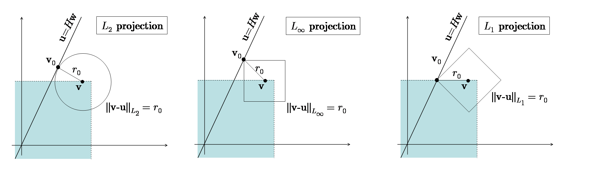
Figure 1. Projections in various norms. The vector $\mathbf{v}$ is projected onto the image space of $H$, i.e., the subspace defined by $\mathbf{u}=H\mathbf{w}$. Consider the smallest sphere around $\mathbf{v}$ (in the corresponding norm) that touches the subspace $\mathbf{u}=H\mathbf{w}$ (shown in each figure). The radius $r_{0}$ of this sphere is the distance of $\mathbf{v}$ from the subspace, and the tangent point $\mathbf{v}_{0}$ (which is not necessarily unique for $L_{1}$ projection) is the projection of $\mathbf{v}$. For this point, $\mathbf{v}_{0}=H\mathbf{w}_{0}$ holds. The shaded region indicates the region $\{\mathbf{u}:\|\mathbf{u}\|_{\infty}\leq\|\mathbf{v}\|_{\infty}\}$. To ensure the convergence of FVI, the projected vector $\mathbf{v}_{0}$ must fall into the shaded region.

Consider the example $\mathbf{v}=[1,1]^{T}\in\mathbb{R}^{2}$, $H=[1,2]^{T}$, $\mathbf{w}\in\mathbb{R}^{1}$. For these values easy calculation shows that $\|H[\mathbf{w}_{0}]_{L_{2}}\|_{\infty}=6/5$ and $\|H[\mathbf{w}_{0}]_{L_{\infty}}\|_{\infty}=4/3,$ i.e., $\|H\mathbf{w}_{0}\|_{\infty}\nleq\|\mathbf{v}\|_{\infty}$ for both cases. For $p=1$, we shall prove the following lemma:

Lemma A.1.

If $\mathbf{w}_{0}=\arg\min_{\mathbf{w}}\|H\mathbf{w}-\mathbf{v}\|_{1}$, then $\|H\mathbf{w}_{0}\|_{\infty}\leq\|\mathbf{v}\|_{\infty}$.

Proof.

Let $\mathbf{z}:=H\mathbf{w}_{0}\in\mathbb{R}^{N}$. If there are multiple solutions to the minimization task, then consider the (unique) $\mathbf{z}$ vector with minimum $L_{2}$-norm. Let $r:=\|\mathbf{z}-\mathbf{v}\|_{1}$ and let $S(\mathbf{v},r)$ be the $L_{1}$-sphere with center $\mathbf{v}$ and radius $r$ (this is an $N$-dimensional cross polytope or orthoplex, a generalization of the octahedron).

Suppose indirectly that $\|\mathbf{z}\|_{\infty}>\|\mathbf{v}\|_{\infty}$. Without loss of generality we may assume that $z_{1}$ is the coordinate of $\mathbf{z}$ with the largest absolute value, and that it is positive. Therefore, $z_{1}>\|\mathbf{v}\|_{\infty}$. Let $\mathbf{e}_{i}$ denote the $i^{\scriptsize\textrm{th}}$ coordinate vector ($1\leq i\leq N$), and let $\mathbf{z}_{\delta}=\mathbf{z}-\delta\mathbf{e}_{1}$. For small enough $\delta$, $S(\mathbf{z}_{\delta},\delta)$ is a cross polytope such that (a) $S(\mathbf{z}_{\delta},\delta)\subset S(\mathbf{v},r)$, (b) $\forall\mathbf{z}^{\prime}\in S(\mathbf{z}_{\delta},\delta)$, $\|\mathbf{z}^{\prime}\|_{\infty}>\|\mathbf{v}\|_{\infty}$, (c) $\forall\epsilon>0$ sufficiently small, $(1-\epsilon)\mathbf{z}\in S(\mathbf{z}_{\delta},\delta)$. The first two statements are trivial. For the third statement, note that $\mathbf{z}$ is a vertex of the cross polytope $S(\mathbf{z}_{\delta},\delta)$. Consider the cone whose vertex is $\mathbf{z}$ and its edges are the same as the edges of $S(\mathbf{z}_{\delta},\delta)$ joining $\mathbf{z}$. It is easy to see that the vector pointing from $\mathbf{z}$ to the origo is contained in this cone: for each $1<i\leq N$, $|z_{i}|\leq z_{1}$ (as $z_{1}$ is the largest coordinate). Consequently, for small enough $\epsilon$, $\mathbf{z}-\epsilon\mathbf{z}\in S(\mathbf{z}_{\delta},\delta)$.

Fix such an $\epsilon$ and let $\mathbf{q}=(1-\epsilon)\mathbf{z}$. This vector is (a) contained in the image space of $H$ because $H[(1-\epsilon)\mathbf{w}]=\mathbf{q}$; (b) $\|\mathbf{q}-\mathbf{v}\|_{1}\leq\|\mathbf{z}-\mathbf{v}\|_{1}=r$. The vector $\mathbf{z}$ was chosen so that it has the smallest $L_{1}$-norm in the image space of $H$, so the inequality cannot be sharp, i.e., $\|\mathbf{q}-\mathbf{v}\|_{1}=r$. However, $\|\mathbf{q}\|_{2}=(1-\epsilon)\|\mathbf{z}\|_{2}<\|\mathbf{z}\|_{2}$ with strict inequality, which contradicts our assumption about $\mathbf{z}$, thus completing the proof. ∎

A.2. Probabilistic interpretation of $N(H^{T})$

Definition A.2.

The basis functions $\{h_{k}\}_{k=1}^{n_{b}}$ have the uniform covering (UC) property, if all row sums in the corresponding $H$ matrix are identical:

$$\sum_{k=1}^{n_{b}}H_{\mathbf{x},k}=B\qquad\textrm{for all $\mathbf{x}\in\mathbf{X}$},$$

and all entries are nonnegative. Without loss of generality we may assume that all rows sum up to 1, i.e., $H$ is a stochastic matrix.

We shall introduce an auxiliary MDP $\overline{\mathcal{M}}$ such that exact value iteration in $\overline{\mathcal{M}}$ is identical to the approximate value iteration in the original MDP $\mathcal{M}$. Let $\mathbf{S}$ be an $K$-element state space with states $\mathbf{s}_{1},\ldots,\mathbf{s}_{K}$. A state $\mathbf{s}$ is considered a discrete observation of the true state of the system, $\mathbf{x}\in\mathbf{X}$.

The action space $A$ and the discount factor $\gamma$ are identical to the corresponding items of $\mathcal{M}$, and an arbitrary element $\mathbf{s}_{0}\in\mathbf{S}$ is selected as initial state. In order to obtain the transition probabilities, let us consider how one can get from observing $\mathbf{s}$ to observing $\mathbf{s}^{\prime}$ in the next time step: from observation $\mathbf{s}$, we can infer the hidden state $\mathbf{x}$ of the system; in state $\mathbf{x}$, the agent makes action $a$ and transfers to state $\mathbf{x}^{\prime}$ according to the original MDP; after that, we can infer the probability that our observation will be $\mathbf{s}^{\prime}$, given the hidden state $\mathbf{x}^{\prime}$. Consequently, the transition probability $\overline{P}(\mathbf{s}^{\prime}\mid\mathbf{s},a)$ can be defined as the total probability of all such paths:

$$\overline{P}(\mathbf{s}^{\prime}\mid\mathbf{s},a):=\sum_{\mathbf{x},\mathbf{x}^{\prime}\in\mathbf{X}}\Pr(\mathbf{x}\mid\mathbf{s})\Pr(\mathbf{x}^{\prime}\mid\mathbf{x},a)\Pr(\mathbf{s}^{\prime}\mid\mathbf{x}).$$

Here the middle term is just the transition probability in the original MDP, the rightmost term is $H_{\mathbf{x},\mathbf{s}}$, and the leftmost term can be rewritten using Bayes’ law (assuming a uniform prior on $\mathbf{x}$):

$$\Pr(\mathbf{x}\mid\mathbf{s}) = \frac{\Pr(\mathbf{s}\mid\mathbf{x})\Pr(\mathbf{x})}{\sum_{\mathbf{x}^{\prime\prime}\in\mathbf{X}}\Pr(\mathbf{s}\mid\mathbf{x}^{\prime\prime})\Pr(\mathbf{x}^{\prime\prime})}=\frac{H_{\mathbf{x},\mathbf{s}}\cdot\frac{1}{|\mathbf{X}|}}{\sum_{\mathbf{x}^{\prime\prime}\in\mathbf{X}}H_{\mathbf{x}^{\prime\prime},\mathbf{s}}\cdot\frac{1}{|\mathbf{X}|}}=\frac{H_{\mathbf{x},\mathbf{s}}}{\sum_{\mathbf{x}^{\prime\prime}\in\mathbf{X}}H_{\mathbf{x}^{\prime\prime},\mathbf{s}}}.$$

Consequently,

$$\overline{P}(\mathbf{s}^{\prime}\mid\mathbf{s},a)=\sum_{\mathbf{x},\mathbf{x}^{\prime}\in\mathbf{X}}\frac{H_{\mathbf{x},\mathbf{s}}}{\sum_{\mathbf{x}^{\prime\prime}\in\mathbf{X}}H_{\mathbf{x}^{\prime\prime},\mathbf{s}}}P(\mathbf{x}^{\prime}\mid\mathbf{x},a)H_{\mathbf{x},\mathbf{s}}=\bigl{[}\mathcal{N}(H)^{T}P^{a}H\bigr{]}_{\mathbf{s},\mathbf{s}^{\prime}}.$$

The rewards can be defined similarly:

$$\overline{R}(\mathbf{s},a):=\sum_{\mathbf{x}\in\mathbf{X}}\Pr(\mathbf{x}\mid\mathbf{s})R(\mathbf{x},a)=\bigl{[}\mathcal{N}(H)^{T}\mathbf{r}^{a}\bigr{]}_{\mathbf{s}}.$$

It is easy to see that approximate value iteration in $\mathcal{M}$ corresponds to exact value iteration in the auxiliary MDP $\overline{\mathcal{M}}$.

A.3. The proof of the sampling theorem (theorem 3.1)

First we prove a useful lemma about approximating the product of two large matrices. Let $A\in\mathbb{R}^{m\times n}$ and $B\in\mathbb{R}^{n\times k}$ and let $C=A\cdot B$. Suppose that we sample columns of $A$ uniformly at random (with repetition), and we also select the corresponding rows of $B$. Denote the resulting matrices with $\widehat{A}$ and $\widehat{B}$. We will show that $A\cdot B\approx c\cdot\widehat{A}\cdot\widehat{B}$, where $c$ is a constant scaling factor compensating for the dimension decrease of the sampled matrices. The following lemma is similar to Lemma 11 of [11], but here we estimate the infinity-norm instead of the $L_{2}$-norm.

Lemma A.3.

Let $A\in\mathbb{R}^{m\times N}$, $B\in\mathbb{R}^{N\times k}$ and $C=A\cdot B$. Let $N^{\prime}$ be an integer so that $1\leq N^{\prime}\leq N$, and for each $i\in\{1,\ldots,N^{\prime}\}$, let $r_{i}$ be an uniformly random integer from the interval $[1,N]$. Let $\widehat{A}\in\mathbb{R}^{m\times N^{\prime}}$ be the matrix whose $i^{\scriptsize\textrm{th}}$ column is the $r_{i}{}^{\scriptsize\textrm{th}}$ column of $A$, and denote by $\widehat{B}$ the $N^{\prime}\times k$ matrix that is obtained by sampling the rows of $B$ similarly. Furthermore, let

$$\widehat{C}=\frac{N}{N^{\prime}}\widehat{A}\cdot\widehat{B}=\frac{N}{N^{\prime}}\sum_{i=1}^{N^{\prime}}A_{*,r_{i}}B_{r_{i},*}.$$

Then, for any $\epsilon,\delta>0$, $\|\widehat{C}-C\|_{\infty}\leq\epsilon N\|A\|_{\infty}\|B^{T}\|_{\infty}$ with probability at least $1-\delta$, if the sample size satisfies $N^{\prime}\geq\frac{2m^{2}}{\epsilon^{2}}\log\frac{2km}{\delta}$.

Proof.

We begin by bounding individual elements of the matrix $\widehat{C}$: consider the element

$$\widehat{C}_{pq}=\frac{N}{N^{\prime}}\sum_{i=1}^{N^{\prime}}A_{p,r_{i}}B_{r_{i},q}.$$

Let $\mathcal{C}_{pq}$ be the discrete probability distribution determined by mass points $\{A_{p,i}\cdot B_{i,q}\mid 1\leq i\leq N\}$. Note that $\widehat{C}_{pq}$ is essentially the sum of $N^{\prime}$ random variables drawn uniformly from distribution $\mathcal{C}_{pq}$. Clearly,

$$|A_{pi}B_{iq}| \leq \max_{ij}|A_{ij}|\max_{ij}|B_{ij}|\leq\max_{i}\sum_{j}|A_{ij}|\max_{i}\sum_{j}|B_{ij}|=\|A\|_{\infty}\|B\|_{\infty},$$

so we can apply Hoeffding’s inequality to obtain

$$\Pr\Bigl{(}\left|\frac{\sum_{i=1}^{N^{\prime}}A_{p,r_{i}}B_{r_{i},q}}{N^{\prime}}-\frac{\sum_{j=1}^{N}A_{p,j}B_{j,q}}{N}\right|>\epsilon_{1}\Bigr{)}<2\exp\Bigl{(}-\frac{N^{\prime}\epsilon_{1}^{2}}{2\|A\|_{\infty}^{2}\|B\|_{\infty}^{2}}\Bigr{)},$$

or equivalently,

$$\Pr\Bigl{(}\left|\frac{N}{N^{\prime}}[\widehat{A}\widehat{B}]_{pq}-[AB]_{pq}\right|>N\epsilon_{1}\Bigr{)}<2\exp\Bigl{(}-\frac{N^{\prime}\epsilon_{1}^{2}}{2\|A\|_{\infty}^{2}\|B\|_{\infty}^{2}}\Bigr{)},$$

where $\epsilon_{1}>0$ is a constant to be determined later. From this, we can bound the row sums of $\widehat{C}-C$:

$$\Pr\Bigl{(}\sum_{p=1}^{m}\left|\widehat{C}_{pq}-C_{pq}\right|>m\cdot N\epsilon_{1}\Bigr{)}<2m\exp\Bigl{(}-\frac{N^{\prime}\epsilon_{1}^{2}}{2\|A\|_{\infty}^{2}\|B\|_{\infty}^{2}}\Bigr{)},$$

which gives a bound on $\|\widehat{C}-C\|_{\infty}$. This is the maximum of these row sums:

$$\Pr\Bigl{(}\|\widehat{C}-C\|_{\infty}>mN\epsilon_{1}\Bigr{)}=\Pr\Bigl{(}\max_{q}\sum_{p=1}^{m}\left|\widehat{C}_{pq}-C_{pq}\right|>mN\epsilon_{1}\Bigr{)}<2km\exp\Bigl{(}-\frac{N^{\prime}\epsilon_{1}^{2}}{2\|A\|_{\infty}^{2}\|B\|_{\infty}^{2}}\Bigr{)}.$$

Therefore, by substituting $\epsilon_{1}=\epsilon\|A\|_{\infty}\|B\|_{\infty}/m$, the statement of the lemma is satisfied if $2km\exp\Bigl{(}-\frac{N^{\prime}\epsilon^{2}}{2m^{2}}\Bigr{)}\leq\delta,$ i.e, if $N^{\prime}\geq\frac{2m^{2}}{\epsilon^{2}}\log\frac{2km}{\delta}.$ ∎

If both $A$ and $B$ are structured, we can sharpen the lemma to give a much better (potentially exponentially better) bound. For this, we need the following definition:

For any index set $Z$, a matrix $A$ is called $Z$-local-scope matrix, if each column of $A$ represents a local-scope function with scope $Z$.

Lemma A.4.

Let $A^{T}$ and $B$ be local-scope matrices with scopes $Z_{1}$ and $Z_{2}$, and let $N_{0}=n^{|Z_{1}|+|Z_{2}|}$, and apply the random row/column selection procedure of the previous lemma. Then, for any $\epsilon,\delta>0$, $\|\widehat{C}-C\|_{\infty}\leq\epsilon N_{0}\|A\|_{\infty}\|B\|_{\infty}$ with probability at least $1-\delta$, if the sample size satisfies $N^{\prime}\geq\frac{2m^{2}}{\epsilon^{2}}\log\frac{2km}{\delta}$.

Proof.

Fix a variable assignment $\mathbf{x}[Z_{1}\cup Z_{2}]$ on the domain $Z_{1}\cup Z_{2}$ and consider the rows of $A$ that correspond to a variable assignment compatible to $\mathbf{x}[Z_{1}\cup Z_{2}]$, i.e., they are identical to it for components $Z_{1}\cup Z_{2}$ and are arbitrary on

$$W:=\{1,2,\ldots,m\}\setminus(Z_{1}\cup Z_{2}).$$

It is easy to see that all of these rows are identical because of the local-scope property. The same holds for the columns of $B$. All the equivalence classes of rows/columns have cardinality

$$N_{1}:=n^{|W|}=N/N_{0}.$$

Now let us define the $m\times N_{0}$ matrix $A^{\prime}$ so that only one column is kept from each equivalence class, and define the $N_{0}\times k$ matrix $B^{\prime}$ similarly, by omitting rows. Clearly,

$$A\cdot B=N_{1}A^{\prime}\cdot B^{\prime},$$

and we can apply the sampling lemma to the smaller matrices $A^{\prime}$ and $B^{\prime}$ to get that for any $\epsilon,\delta>0$ and sample size $N^{\prime}\geq\frac{2m^{2}}{\epsilon^{2}}\log\frac{2km}{\delta}$, with probability at least $1-\delta$,

$$\|\widehat{A^{\prime}\cdot B^{\prime}}-A^{\prime}\cdot B^{\prime}\|_{\infty}\leq\epsilon N_{0}\|A^{\prime}\|_{\infty}\|B^{\prime}\|_{\infty}.$$

Exploiting the fact that the max-norm of a matrix is the maximum of row norms, $\|A^{\prime}\|_{\infty}=\|A\|_{\infty}/N_{1}$ and $\|B^{\prime}\|_{\infty}=\|B\|_{\infty}$, we can multiply both sides to get

$$\|N_{1}\widehat{A^{\prime}\cdot B^{\prime}}-A\cdot B\|_{\infty}\leq\epsilon N_{0}N_{1}\|A\|_{\infty}/N_{1}\|B\|_{\infty}=\epsilon N_{0}\|A\|_{\infty}\|B\|_{\infty},$$

which is the statement of the lemma. ∎

Note that if the scopes $Z_{1}$ and $Z_{2}$ are small, then the gain compared to the previous lemma can be exponential.

Lemma A.5.

Let $A=A_{1}+\ldots+A_{p}$ and $B=B_{1}+\ldots+B_{q}$ where all $A_{i}$ and $B_{j}$ are local-scope matrices with domain size at most $z$, and let $N_{0}=n^{z}$. If we apply the random row/column selection procedure, then for any $\epsilon,\delta>0$, $\|\widehat{C}-C\|_{\infty}\leq\epsilon N_{0}pq\max_{i}\|A_{i}\|_{\infty}\max_{j}\|B_{j}\|_{\infty}$ with probability at least $1-\delta$, if the sample size satisfies $N^{\prime}\geq\frac{2m^{2}}{\epsilon^{2}}\log\frac{2km}{\delta}$.

Proof.

$$\|\widehat{C}-C\|_{\infty}\leq\sum_{i=1}^{p}\sum_{j=1}^{q}\|\widehat{A_{i}\cdot B_{j}}-A_{i}\cdot B_{j}\|_{\infty}.$$

For each individual product term we can apply the previous lemma. Note that we can use the same row/column samples for each product, because independence is required only within single matrix pairs. Summing the right-hand sides gives the statement of the lemma. ∎

Now we can complete the proof of Theorem 3.1:

Proof.

$$\|\mathbf{w}^{*}-\mathbf{w}^{\prime}\|_{\infty} = \|G\mathcal{T}H\mathbf{w}^{*}-\widehat{G}\mathcal{T}\widehat{H}\mathbf{w}^{\prime}\|_{\infty}$$

$$\leq \|G\mathcal{T}H\mathbf{w}^{*}-\widehat{G}\mathcal{T}\widehat{H}\mathbf{w}^{*}\|_{\infty}+\|\widehat{G}\mathcal{T}\widehat{H}\mathbf{w}^{*}-\widehat{G}\mathcal{T}\widehat{H}\mathbf{w}^{\prime}\|_{\infty}$$

$$\leq \|G\mathcal{T}H\mathbf{w}^{*}-\widehat{G}\mathcal{T}\widehat{H}\mathbf{w}^{*}\|_{\infty}+\gamma\|\mathbf{w}^{*}-\mathbf{w}^{\prime}\|_{\infty},$$

i.e., $\|\mathbf{w}^{*}-\mathbf{w}^{\prime}\|_{\infty}\leq\frac{1}{1-\gamma}\|G\mathcal{T}H\mathbf{w}^{*}-\widehat{G}\mathcal{T}\widehat{H}\mathbf{w}^{*}\|_{\infty}$. Let $\pi_{0}$ be the greedy policy with respect to the value function $H\mathbf{w}^{*}$. With its help, we can rewrite $\mathcal{T}H\mathbf{w}^{*}$ as a linear expression: $\mathcal{T}H\mathbf{w}^{*}=\mathbf{r}^{\pi_{0}}+\gamma P^{\pi_{0}}H\mathbf{w}^{*}.$ Furthermore, $\mathcal{T}$ is a componentwise operator, so we can express its effect on the downsampled value function as $\mathcal{T}\widehat{H}\mathbf{w}^{*}=\widehat{\mathbf{r}}^{\pi_{0}}+\gamma\widehat{P^{\pi_{0}}H}\mathbf{w}^{*}.$ Consequently,

$$\|G\mathcal{T}H\mathbf{w}^{*}-\widehat{G}\mathcal{T}\widehat{H}\mathbf{w}^{*}\|_{\infty}\leq\|G\mathbf{r}^{\pi_{0}}-\widehat{G}\widehat{\mathbf{r}}^{\pi_{0}}\|_{\infty}+\gamma\|GP^{\pi_{0}}H-\widehat{G}\widehat{P^{\pi_{0}}H}\|_{\infty}\|\mathbf{w}^{*}\|_{\infty}$$

Applying the previous lemma two times, we get that with probability greater than $1-\delta_{1}$, $\|G\mathbf{r}^{\pi_{0}}-\widehat{G}\widehat{\mathbf{r}}^{\pi_{0}}\|_{\infty}\leq\epsilon_{1}C_{1}$ if $N^{\prime}\geq\frac{2m^{2}}{\epsilon_{1}^{2}}\log\frac{2m}{\delta_{1}}$ and with probability greater than $1-\delta_{2}$, $\|GP^{\pi_{0}}H-\widehat{G}\widehat{P^{\pi_{0}}H}\|_{\infty}\leq\epsilon_{2}C_{2}$ if $N^{\prime}\geq\frac{2m^{2}}{\epsilon_{2}^{2}}\log\frac{2m^{2}}{\delta_{2}}$; where $C_{1}$ and $C_{2}$ are constants depending polynomially on $N_{0}$ and the norm of the component local-scope functions, but independent of $N$.

Using the notation $M=\frac{1}{1-\gamma}\Bigl{(}C_{1}+\gamma C_{2}\|\mathbf{w}^{*}\|_{\infty}\Bigr{)}$, $\epsilon_{1}=\epsilon_{2}=\epsilon/M$, $\delta_{1}=\delta_{2}=\delta/2$ and $\Xi=M^{2}$ proves the theorem. ∎

Informally, this theorem tells that the required number of samples grows quadratically with the desired accuracy $1/\epsilon$ and logarithmically with the required certainty $1/\delta$, furthermore, the dependence on the number of variables $m$ is slightly worse than quadratic. This means that even if the number of equations is exponentially large, i.e., $N=O(e^{m})$, we can select a polynomially large random subset of the equations so that with high probability, the solution does not change very much.

References

- [1] Stefan Arnborg, Derek G. Corneil, and Andrzej Proskurowski. Complexity of finding embeddings in a k-tree. SIAM Journal on Algebraic and Discrete Methods, 8(2):277–284, 1987.
- [2] L.C. Baird. Residual algorithms: Reinforcement learning with function approximation. In ICML, pages 30–37, 1995.
- [3] Richard E. Bellman. Adaptive Control Processes. Princeton University Press, Princeton, NJ., 1961.
- [4] D.P. Bertsekas and J.N. Tsitsiklis. Neuro-Dynamic Programming. Athena Scientific, 1996.
- [5] C. Boutilier, R. Dearden, and M. Goldszmidt. Exploiting structure in policy construction. In IJCAI, pages 1104–1111, 1995.
- [6] Craig Boutilier, Richard Dearden, and Moises Goldszmidt. Stochastic dynamic programming with factored representations. Artificial Intelligence, 121(1-2):49–107, 2000.
- [7] D.P. de Farias and B. van Roy. Approximate dynamic programming via linear programming. In NIPS, pages 689–695, 2001.
- [8] D.P. de Farias and B. van Roy. On constraint sampling in the linear programming approach to approximate dynamic programming. Mathematics of Operations Research, 29(3):462–478, 2004.
- [9] R. Dechter. Bucket elimination: A unifying framework for reasoning. AIJ, 113(1-2):41–85, 1999.
- [10] Dmitri A. Dolgov and Edmund H. Durfee. Symmetric primal-dual approximate linear programming for factored MDPs. In Proceedings of the 9th International Symposium on Artificial Intelligence and Mathematics (AI&M 2006), 2006.
- [11] P. Drineas, R. Kannan, and M.W. Mahoney. Fast Monte Carlo algorithms for matrices I: Approximating matrix multiplication. SIAM Journal of Computing, 36:132–157, 2006.
- [12] P. Drineas, M.W. Mahoney, and S. Muthukrishnan. Sampling algorithms for l2 regression and applications. In SODA, pages 1127–1136, 2006.
- [13] C. Guestrin, D. Koller, R. Parr, and S. Venkataraman. Efficient solution algorithms for factored MDPs. JAIR, 19:399–468, 2002.
- [14] C. Guestrin, R. Patrascu, and D. Schuurmans. Algorithm-directed exploration for model-based reinforcement learning in factored mdps. In ICML, pages 235–242, 2002.
- [15] Carlos Guestrin, Daphne Koller, Chris Gearhart, and Neal Kanodia. Generalizing plans to new environments in relational MDPs. In Eighteenth International Joint Conference on Artificial Intelligence, 2003.
- [16] M.J. Kearns and D. Koller. Efficient reinforcement learning in factored MDPs. In Proceedings of the 16th International Joint Conference on Artificial Intelligence, pages 740–747, 1999.
- [17] D. Koller and R. Parr. Policy iteration for factored MDPs. In UAI, pages 326–334, 2000.
- [18] Branislav Kveton, Milos Hauskrecht, and Carlos Guestrin. Solving factored MDPs with hybrid state and action variables. Journal of Artificial Intelligence Research, 27:153–201, 2006.
- [19] M.G. Lagoudakis and R. Parr. Least-squares policy iteration. JMLR, 4:1107–1149, 2003.
- [20] P. Liberatore. The size of MDP factored policies. In AAAI, pages 267–272, 2002.
- [21] Relu Patrascu, Pascal Poupart, Dale Schuurmans, Craig Boutilier, and Carlos Guestrin. Greedy linear value-approximation for factored markov decision processes. In Proceedings of the 18th National Conference on Artificial intelligence, pages 285–291, 2002.
- [22] Pascal Poupart, Craig Boutilier, Relu Patrascu, and Dale Schuurmans. Piecewise linear value function approximation for factored mdps. In Proceedings of the 18th National Conference on AI, 2002.
- [23] Brian Sallans. Reinforcement Learning for Factored Markov Decision Processes. PhD thesis, University of Toronto, 2002.
- [24] Scott Sanner and Craig Boutilier. Approximate linear programming for first-order MDPs. In Proceedings of the 21th Annual Conference on Uncertainty in Artificial Intelligence (UAI), pages 509–517, 2005.
- [25] P.J. Schweitzer and A. Seidmann. Generalized polynomial approximations in Markovian decision processes. Journal of Mathematical Analysis and Applications, 110(6):568–582, 1985.
- [26] R.S. Sutton and A.G. Barto. Reinforcement Learning: An Introduction. MIT Press, 1998.
- [27] John N. Tsitsiklis and Benjamin Van Roy. An analysis of temporal-difference learning with function approximation. IEEE Transactions on Automatic Control, 42(5):674–690, 1997.