Predictability in Semi-Analytic Models of Galaxy Formation

Abstract

We propose a general framework to scrutinize the performance of semi-analytic codes of galaxy formation. The approach is based on the analysis of the outputs from the model after a series of perturbations in the input parameters controlling the baryonic physics. The perturbations are chosen in a way that they do not change the results in the luminosity function or mass function of the galaxy population.

We apply this approach on a particular semi-analytic model called GalICS. We chose to perturb the parameters controlling the efficiency of star formation and the efficiency of supernova feedback. We keep track of the baryonic and observable properties of the central galaxies in a sample of dark matter halos with masses ranging from $10^{10}$ M_⊙ to $10^{13}$ M_⊙.

We find very different responses depending on the halo mass. For small dark matter halos its central galaxy responds in a highly predictable way to small perturbation in the star formation and feedback efficiency. For massive dark matter halos, minor perturbations in the input parameters can induce large fluctuations on the properties of its central galaxy, at least $\sim 0.1$ in $B-V$ color or $\sim 0.5$ mag in $U$ or $r$ filter, in a seemingly random fashion. We quantify this behavior through an objective scalar function we call predictability.

We argue that finding the origin of this behavior needs additional information from other approximations and different semi-analytic codes. Furthermore, the implementation of an scalar objective function, such as the predictability, opens the door to quantitative benchmarking of semi-analytic codes based on its numerical performance.

1 Introduction

Hierarchical aggregation seems to be at the heart of galaxy evolution. In a cold dark matter universe, as depicted by numerical simulations, its structure grows through subsequent mergers and zero fragmentations. The growth and evolution of galaxies, which are thought to use dark matter as scaffolding, is channeled through this hierarchical aggregation, at least for the most massive structures (Springel et al., 2006).

Notwithstanding all the complexity in the process of galaxy formation and evolution, galaxies still are the most basic population unit in the description of large scale structure in the Universe. And still nowadays much work is being invested in galaxy formation to disentangle the influence of the hierarchical context setup by dark matter from the secular baryonic processes on small scales.

Tackling the problem theoretically implies numerical experiments following large structure dynamics and, at the same time, a description of baryonic processes such hydrodynamics and radiative cooling. This is still very challenging in the usual numerical approach that discretizes space and time, and try to solve a relevant set of equations to capture the physics (Abel et al., 2002; Gottlöber et al., 2006). From the computational point of view it involves achieving an effective resolution spanning at least $5$ orders of magnitude in mass, length and time (Norman et al., 2007).

To overcome this barrier the semi-analytic model (hereafter SAM) approach proposes to describe first the non-linear clustering of dark matter on large scales, and describe later the small scale baryonic physics through analytical prescriptions. The connection between the two scales is provided through the dark matter halo, which is the most basic unit of non-linear dark matter structure (see Baugh (2006) and references therein).

The non linear clustering of dark matter is described through a merger tree, representing the merging history of a given dark matter halo. The construction methods for merger trees can vary, ranging from Monte-Carlo realizations based on theoretical estimates (Somerville & Kolatt, 1999) to the numerical based on N-body simulations (Croton et al., 2006), including also hybrid approaches mixing numerical and analytical techniques (Taffoni et al., 2002).

The different analytic implementations of baryonic process span a wide range of philosophical approaches, physical concepts and numerical implementations. Most of them, nonetheless, constructed from observed correlations in our local patch of Universe.

Regardless of the details of these models, what is general to all of them is the underlying merger trees structure complementary with analytic recipes describing the growth of baryonic structure inside the merger trees. The ignorance respect to the physics included in the analytic recipes is usually represented by scalars, which in most of the cases represent efficiencies of physical processes. This implies that a given realization of a semi-analytic run is completely determined by the dark matter input and the baryonic parameters in the simulation.

Most of the work during the last decade was invested in adding and exploring the effect of these parameters on average quantities, especially the luminosity function. The generic parameters to be used have been more or less settled, and most of the models have achieved a good level of internal consistency by reproducing some key observational features. The confidence on the consistency that can be achieved, and the ease to perform a semi-analytic run, have empowered the modelers to select subsamples and make studies about the most massive galaxies or correlations among populations (De Lucia & Blaizot, 2007; Hayashi & White, 2007).

As the complexity and interest in semi analytic techniques grow, two relevant issues must be addressed in more detail. First, the issue of error propagation from the incertitude in the input parameters, a factor that might be important in a hierarchical Universe, where the amplification of small initial errors might be important for the most massive and hierarchical objects. Second, the development of objective ways to compare different types of complexity in semi analytic models. This could allow, for instance, the implementation of simple tests with an objective scalar function to measure the model performance.

The objective of this paper is two-fold:

• Propose a methodology to weigh the role of secular baryonic processes in the context of SAMs.

• Propose an objective scalar function that captures the biases and general behavior of semi-analytic models regardless of its detailed implementation.

These two objectives are a result of the same perturbative approach we advocate in this paper. This approach is based on the fact that the only objective information we have to describe the results of a semi-analytic run are the input parameters of the model. In the perturbative approach, we perform semi-analytic runs in the neighborhood of some scalar parameters. This will allow us, as we will show, to get an idea about the limits of our semi-analytic model.

This paper is structured as follows. In Section 2 we describe the structure common to all SAMs and from that point we introduce the concept of perturbations in a semi-analytic model. In Section 3 we introduce the setup for the perturbation experiment of our SAM. We describe in Section 4 the two most relevant qualitative features of the experiment results. We select one of this qualitative results to make a detailed quantitative analysis with three different indices, these results are shown in Section 5. We discuss our results in Section 6.

2 Semi-Analytic Models

2.1 Common features

Semi-analytic models exploit the fact that there are two very different physical scales involved in the process of galaxy formation and evolution. On large scales dark matter and gravity are dominant, while on smaller scales complex radiative processes are central to the development of galactic sized structures (Somerville & Primack, 1999; Hatton et al., 2003; Bell et al., 2003; Croton et al., 2006; Monaco et al., 2007).

Inside semi-analytic models all the non-linear dark matter dynamic is described through the merger tree, which represent the process of successive mergers building a dark matter halo. On top of this merger tree, all the complex baryonic physics are implemented through analytic prescriptions derived in most part from observations.

The baryonic processes, in the end, are controlled by a set of scalars, which represent most of the time either an efficiency or a threshold value. From the pure functional point of view, all the baryonic properties $\mathcal{B}$ of a dark matter halo $\mathcal{H}$ are a function of its merger tree $\mathcal{T}$ and the set of scalar parameters controlling the model $\{\lambda_{1}\ldots\lambda_{N}\}$.

$$\mathcal{B}=\mathcal{B}(\mathcal{T},\lambda_{1},\ldots,\lambda_{N}).$$ (1)

Furthermore, during a semi-analytic run, the set of parameter $\{\lambda_{1}\ldots\lambda_{N}\}$ is fixed to be the same for all the halos, all the time. Thus, the trees and the scalar values completely define the outputs.

From the perspective of disentangling the role of different physical elements in the process of galaxy formation, the approach commonly followed is the exploration through a set of different values for the $\{\lambda_{i}\}$ parameters, taking as a gauge the reproduction of the luminosity function of diverse galaxy populations. This coarse exploration of parameter space have been done until a minimum internal consistency is achieved, a decision based on the success of reproducing a wide set of observational constraints.

Nowadays more and more results of semi-analytic models are being used in the predictive sense, selecting subsamples of galaxies, trying to explain or predict astrophysical quantities of interest based on the results of a semi-analytic model (De Lucia & Blaizot, 2007; Hayashi & White, 2007). This have been done without an explicit treatment of the potential biases and complications introduced by the semi-analytic model itself.

We are interested in understanding in greater detail the behavior and limits of semi-analytic methods, regardless of its detailed implementation across different codes. Our attempt to deal with the complexity across semi-analytic models, is based on the basic conceptual approach in Eq.1, which is the only structural information we have about how semi-analytic models work.

2.2 Perturbing the model

We intend to measure the effect of perturbations in the model

$$\mathcal{B}^{\prime}=\mathcal{B}(\mathcal{T},\lambda_{1}+\delta\lambda_{1},\ldots,\lambda_{N}+\delta\lambda_{N}),$$ (2)

where the magnitudes of the perturbations $\delta\lambda_{i}$ are constrained in such a way that its effect is not significant on the mean population quantities such as the luminosity function, meaning that we are not breaking the broad consistency of the model.

The main objective is measuring the consequences of these perturbation and to use them as a gauge of the model’s numerical performance, but also to see how and where are going to emerge the consequences of the perturbations.

If we intend to explore the neighborhood of a given set of parameters $\{\lambda_{i}\}$ by making runs around $\{\pm\delta\lambda_{i}\}$, this implies performing $2^{N}$ different runs where $N$ is the total number of scalar parameters controlling the model. If we want to explore the neighborhood around $m$ different values for each $\lambda_{i}$, the number of runs becomes $m^{N}$.

The number of free parameters in SAMs can be at least $6$. Which means that we should deal at least with $2^{6}=64$ different runs to minimally explore the neighborhood of $\{\lambda_{i}\}$. Performing all these runs over a cosmological volume is unfeasible and perhaps not very useful.

The approach we decided to follow in this paper uses two simplifications. First, we only perform the simulations over a subset of dark matter halos selected at random in a box of cosmological size. Second, we explore only the neighborhood of two scalar parameters.

The size of the halo subsample is about $1\%$ of the total number of halos in the simulated cosmological box, and the parameters we will explore are the star formation efficiency $\alpha$ and the supernova feedback efficiency $\epsilon$.

3 Experiment

The semi-analytic model we use in this paper is a slightly modified version of that presented in Hatton et al. (2003). As we do not want to compare our results with observations or another models, we briefly review only the elements relevant for our discussion: the dark matter description and the star formation and supernovae feedback implementations.

3.1 Dark Matter

The dark matter simulation was performed using cosmological parameters compatible with a 1st year WMAP cosmology (Spergel et al., 2003) ($\Omega_{m}$, $\Omega_{\Lambda}$, $\sigma_{8}$, $h$) $=$ ($0.30$, $0.70$, $0.92$, $0.70$), where the parameters stand for the density of matter, density of dark energy, amplitude of the mass density fluctuations and the Hubble constant in units of $100$ km s^-1 Mpc ^-1. . The simulation volume is a cubic box of side $100h^{-1}$ Mpc with $512^{3}$ dark matter particles, which sets the mass of each particle to $5.16\times 10^{8}\ h^{-1}$ M_⊙. The simulation was evolved from an initial redshift $z=32$ down to redshift $z=0$, keeping the particle data for $100$ time-steps.

For each recorded timestep build a halo catalogue using a friends-of-friends algorithm (Davis et al., 1985) with linking length $b=0.2$. Only the groups with $20$ or more bound particles are identified as halos. This sets the minimal mass for a dark matter halo to $1.03\times 10^{10}\ h^{-1}$ M_⊙. These halo catalogues provide the input for the construction of the merger trees used as input for the semi-analytic model.

3.2 Star Formation and SN feedback

The star formation rate is set proportional proportional to the mass of cold gas, and without any other characteristic time scale we impose that the rate at which the gas is consumed to form stars is given by the dynamical time of the disc. This is motivated by the observational correlations observed by Kennicutt-Schmidt (Kennicutt, 1998).

Hence, in our model, the global star formation rate $\Psi_{\star}$ on galactic scales is given by the following equation

$$\Psi_{\star}=\alpha\frac{m_{gas}}{t_{dyn}},$$ (3)

where $\alpha$ is an efficiency parameter, and $t_{dyn}$ is the dynamical timescale of the component we are interested (disc or bulge). For $t_{dyn}$ we use the time taken for material at the half-mass radius to reach either the opposite side of the galaxy (disc) or its center (bulge), and is given by:

$$t_{dyn}=r_{1/2}\times\pi v^{-1},$$ (4)

where $v$ is a characteristic velocity in the galaxy component and $r_{1/2}$ is the half mass radius. For discs the velocity $v$ is equal to the circular velocity of the disc where the material is assumed to have purely circular orbits. In the case of spheroidal components $v$ is the velocity dispersion, where we assume the matter in the component has only radial orbits.

The star formation is triggered if the column density of the gas is greater that a given threshold constrained by the observations Kennicutt (1998). By simplicity we assume that the initial mass function is universal at all redshift and follows a Kennicutt initial mass function.

Once stars are formed, the massive stars will explode inside the galaxies ejecting hot gas and metals in the interstellar medium. The simple model that we use for this phenomenon is given by the implementation of Silk (2001), where the rate of gas mass loss is written assuming an stationary model

$$\frac{dm_{out}}{dt}=\Psi_{\star}\times\eta_{SN}\Delta m_{SN}\times(1+L)\times(1-e^{-R}),$$ (5)

where $\Psi_{\star}$ is the star formation rate, $\eta_{SN}$ is the number of supernovae per unit mass of formed stars (fixed number function of the IMF), $\Delta m_{SN}$ is mean mass loss of one supernova ($\sim 10$ M_⊙) and $(1+L)$ is defined as

$$1+L\equiv\epsilon\frac{m_{gas}}{m_{gal}},$$ (6)

where $m_{gas}$ and $m_{gal}$ are the gas and total mass of the galaxy component and the parameter $\epsilon$ regulates the efficiency of the feedback. We also define the porosity of the galaxy component as

$$R=\alpha\left(\frac{m_{gal}}{m_{gas}}\right)^{1/2}\left(\frac{17.8}{\sigma}\right)^{2.72},$$ (7)

where $\sigma$ is a typical dispersion velocity in the interstellar medium (in km/s), which we fix to $10$km/s for disks and to the velocity dispersion for the spheroidal components. The parameter $\alpha$ is the star formation efficiency. In this model, usually the ejected amount of gas is of the same order of the mass of formed stars.

3.3 Experiment Setup

From the detected halos at redshift zero we select at random nearly $600$ of them, which corresponds to about $1\%$ of the total number of halos in the box. For each halo we have its corresponding merger history, and we are able to run our galaxy formation code on every individual merger tree.

For each halo we make 320 runs varying two parameters, the star formation efficiency $\alpha$ and the supernova feedback efficiency $\epsilon$. The first parameter, $\alpha$, is sampled at 16 points between 0.018 and 0.022, and the second, $\epsilon$, is sampled at 20 points between 0.18 and 0.20. From this we define a 2-dimensional representation to keep track of each run. We setup two coordinate plane. Along the first dimension ($x$-axis) we vary the star formation efficiency $\alpha$, and along the second dimension ($y$-axis) we vary the supernova feedback efficiency $\epsilon$. This defines the $\alpha$-$\epsilon$ plane.

For each run (for a given halo and for given point in the $\alpha$-$\epsilon$ plane) we select the central galaxy in the halo, which is the only galaxy with a clear identity in a hierarchical paradigm. For each central galaxy we track six physical properties: total mass (gas and stars), mass of stars , bolometric luminosity, absolute magnitude in the SDSS_U, SDSS_r filters and the $B-V$ color. We will refer to the values of a given galactic property, for a given galaxy, over the $\alpha$-$\epsilon$ plane as a landscape.

4 Qualitative Results

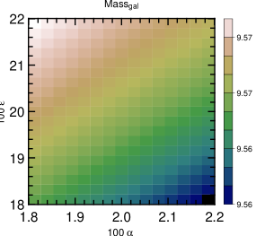
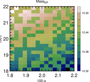
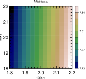
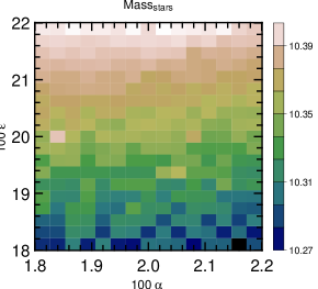
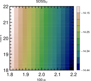
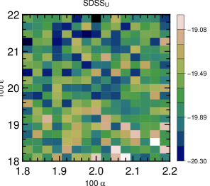
Figure 1: Results for the sampling of the star formation efficiency $\alpha$ and the supernova feedback efficiency $\epsilon$. Each panel represents the results of some galactic property in the central galaxy of a dark matter halo. On the left, the results correspond to the central galaxy in a halo of mass $\sim 10^{10}$ M_⊙. On the right, to a more massive halo of $\sim 10^{12}$ M_⊙. For each galaxy we show the results concerning the total galaxy mass (upper panels), the stellar mass (middle panels) and the magnitude in the SDSS_U band (lower panels). Every small square in each panel shows the result at redshift $z=0$ for the run with the corresponding value of $\alpha$ and $\epsilon$. The results for the low mass halo are predictable, for the high mass halo they are almost random. Note that for instance in the case of the SDSS_U filter the values fluctuate over a range of $\sim 1.4$ mag. The bulk of our paper is devoted to the quantification of this behavior as a function of halo mass.

Figure 2: Histograms (normalized to add up to unity) of the values over four randomly selected the landscapes. From left to right the mass of the host dark matter halo increases. Upper row shows the results for the SDSS_U magnitudes. Lower row: SDSS_r magnitudes. This illustrates another qualitative feature of the landscapes, namely that sometimes they are bimodal, for instance in the upper-left panel. We do not try to quantify this behavior in the paper.

We present in Fig.1 the landscapes for the total galactic mass, stellar mass and SDSS_U absolute magnitude for two galaxies, each column representing one galaxy. Qualitatively speaking, we can spot a striking difference in this figure.

The left column in Fig.1 presents the results for a central galaxy in halo of mass $\sim 10^{11}$M_⊙. Its growth process have been dominated by what we call smooth accretion, meaning that at our working resolution this halo has not suffered any major merger. The predicted properties vary smoothly over the $\alpha$-$\epsilon$ plane.

On the right column in the same figure, we show the same properties for the central galaxy in a halo of mass $\sim 10^{13}$M_⊙. In this case the values over the landscape do not follow any pattern. The biggest difference with respect to the previous case is that the halo growth cannot be described by pure accretion, but through repeated mergers.

A second qualitative feature is the emerging bimodality for some landscapes. It is visible in the upper right panel in Fig.1, where it seems that the values over the landscape are oscillating back and forth between two planes. To illustrate better this effect we have constructed the histograms for two kind of landscapes (SDSS_r and SDSS_U magnitudes) for four different halo masses. The results are shown in Fig.2, which shows how the landscapes are not necessarily unimodal. By visual inspection of half of the landscapes for the total mass, bolometric luminosity and SDSS_r, we can report that the non-unimodality is a recurrent landscape feature.

For the rest of the paper we will be concerned with a quantification of the first result, which showed an apparent randomness for the central galaxies in strongly hierarchical halos. We will use three different indicators.

First, we will define a scalar function called predictability, $P$, for a given galactic property over the $\alpha$-$\epsilon$ plane (Pascual & Levin, 1999). The predictability will be almost one for the low mass case, and zero (or even negative) for the case of the massive halo.

The second method of quantification is based on the predictability and the variance over the landscapes. We will calculate a predictability-weighted variance, which is intended to represent a quantitative estimation of the variations we can expect in a galactic property after performing a minimal perturbation $\delta\alpha$-$\delta\epsilon$.

The last method of quantification compares the variance over the landscapes with the variance over a subsample of galaxies hosted by halos of similar mass inside the full cosmological box.

5 Quantitative Results

5.1 Predictability

We present the first part of the qualitatively results using a scalar function we call predictability. First, we sketch out the general idea behind its definition.

We place ourselves on the $\alpha$-$\epsilon$ plane, and we want to predict the value of some galactic quantity at the point we are standing, we also intend to use the information available in the neighborhood. We have the values of the quantity we want to measure for the four nearest neighbors in the $\alpha$ -$\epsilon$ plane. We make a guess for that value by averaging these values, and at the same time we perform the measurement.

We have now two different values at the point in the $\alpha$ -$\epsilon$ plane, one is predicted and the other is measured. If the squared difference between these two values is small for each point in the plane, we can be sure that we are over a smooth landscape. If the squared differences over the plane are big, the landscape is not so smooth. The predictability is a measure based on these squared differences.

In practice, we use a discretization of the plane $\alpha$-$\epsilon$, and we construct two different scalar fields over that plane. The first corresponds to the field measured in the numerical runs, noted $L$. The second is a predicted version, noted $L^{\prime}$.

The values of $L^{\prime}(\alpha_{i},\epsilon_{j})$ are calculated from the neighboring points in $L(\alpha,\epsilon)$, as follows

$$L^{\prime}(\alpha_{i},\epsilon_{j})=\frac{1}{4}[L(\alpha_{i+1},\epsilon_{j})+\\ L(\alpha_{i-1},\epsilon_{j})+L(\alpha_{i},\epsilon_{j+1})+L(\alpha_{i},\epsilon_{j-1})].$$ (8)

We construct now the following quantity

$$Q^{2}=\frac{1}{N}\sum_{i,j}[L^{\prime}(\alpha_{i},\epsilon_{j})-L(\alpha_{i},\epsilon_{j})]^{2},$$ (9)

where $N$ is the total number of points in the plane $\alpha$- $\epsilon$. This quantity help us to define the predictability

$$P=1-\frac{Q^{2}}{\sigma^{2}},$$ (10)

with $\sigma^{2}$ as the variance of the landscape

$$\sigma^{2}=\frac{1}{N}\sum_{i,j}[L(\alpha_{i},\epsilon_{j})-\bar{L}]^{2}.$$ (11)

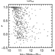
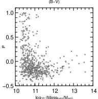
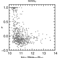
Figure 3: Results for the predictability of different properties. Each point represents a central galaxy. From left to right, top to bottom: total mass of the galaxy, stellar mass, bolometric luminosity, $(B-V)$ color, SDSS_U and SDSS_r magnitudes. The most dependent quantities on the star formation history (colors and magnitudes) are observed in general to have a very low predictability. The most predictable quantity respect to variations in the $\alpha$-$\epsilon$ plane is the total galactic mass.

The predictability is bounded to $P\leq 1$. A value of $P\sim 1$ implies that the landscape is very smooth, while for values $P\leq 0$ the changes from neighboring sites can be high.

We now turn to the results of the Fig.3, where we plot the predictability as a function of the logarithm of the mass of the host halo, for all the galaxies in our study. Starting with the total galaxy mass (stars and the gas) we can see that the galaxies have high predictability, $P>0.9$, in most of the cases. The situation is quite different for the stellar mass and the bolometric luminosity. In these cases the predictability ranges almost evenly between $0<P<1$, and we start seeing some fraction of points with negative predictability. In the case of the $(B-V)$ colors and SDSS_U, SDSS_r magnitudes we are in a totally different ballpark as most of the landscapes have negative predictability, with a few points over the range $0<P<1$.

The conclusion after these results is that we spot a landscape with a very predictability $P<0.9$ we can be sure that the galaxy is sitting in halo less massive than $3\times 10^{11}$ M_⊙. In the same vein, when picking the central galaxy in a halo of mass $>10^{12}$ M_⊙, surely the predictability is going to be lower $P<0.9$, or negative in the case of $(B-V)$ colors and SDSS_r, SDSS_U magnitudes.

5.2 P-Weighted Landscape Variance

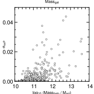
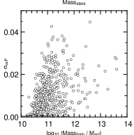
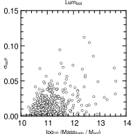
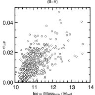
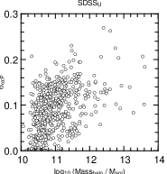
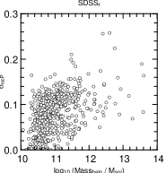
Figure 4: Predictability-weighted variance ($\sigma_{\alpha\epsilon P}$) over the $\alpha$-$\epsilon$ landscape (Eq. 12). This quantity can be used as an estimation of the expected change in a given galactic property when a variation $(\delta\alpha,\delta\epsilon)$ is performed on the input parameters. In the case of magnitudes it can be easily as high as $0.5$ for a $1\%$ variation in $(\alpha,\delta)$. A trend seems to indicate that this weighted variance increases with the dark matter halo mass.

We explore now the second way of quantification of our results. It is based on the landscape variance $\sigma_{\alpha\epsilon}$ over the the 320 points in the $\alpha$-$\epsilon$ plane (Eq.11) and the predictability P (Eq.10).

We want to weight the landscape variance by the information obtained through the predictability $P$. Performing a normalization in this way we can have an idea about how much should be expected to vary a given galactic property after performing a perturbation ($\delta\alpha,\delta\epsilon$).

Using the variance $\sigma_{\alpha\epsilon}$ alone can be misleading in the case of a high predictability landscape, because it could over-estimate the variation of performing a ($\delta\alpha,\delta\epsilon$) perturbation.

We propose then, the $P$-weighted variance

$$\sigma_{\alpha\epsilon P}=(1-e^{P-1})\times\sigma_{\alpha\epsilon},$$ (12)

which has the property of being bound between $0\leq\sigma_{\alpha\epsilon P}\leq\sigma_{\alpha\epsilon}$ for the possible values of the predictability $-\infty<P\leq 1$.

The general trend (Fig.4) shows a growth in the $P$-weighted predictability with halo mass, consistent with the fact that the largest values for the predictability come along with large values for the landscape variance. The results for the total mass landscape and the bolometric luminosity stand apart, as this mass trend is less clear than for the other galactic properties.

The values can be used to measure the variation one can expect from a $1\%$ perturbation in $(\alpha,\epsilon)$. If we recall that this is calculated from a $1$-$\sigma$ variance, the value of $\sigma_{\alpha\epsilon P}$ that could effectively bracket the fluctuations over the $\alpha$-$\epsilon$ plane would be three times that value. It means that for the most massive halos of mass $\sim 10^{13}$ M_⊙ one can expect, at least, a variation of $\sim 0.5$ in the SDSS_U magnitudes or $\sim 0.1$ for the $(B-V)$ colors after $1\%$ variation in $(\alpha,\epsilon)$. The variation in the total and stellar mass could achieve at least $\sim 0.1$ dex.

5.3 Cosmological Variance

Now we compare the landscape variance $\sigma_{\alpha\epsilon}$ with the scale imposed by the cosmological context. We select from the simulated cosmological box (with $\alpha$ and $\epsilon$ in the center of the $\alpha$-$\epsilon$ plane) all the dark matter halos with the same mass (within $1\%$) as the parent halo of the galaxy under study. From this halo population, we calculate the variance $\sigma_{halo}$ of the galactic properties of our interest for its central galaxies.

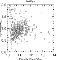
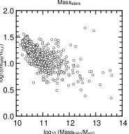
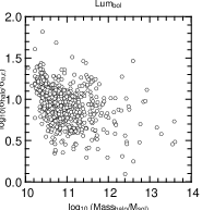
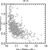
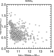
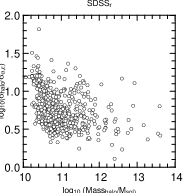
Figure 5: Logarithm of the ratio of the variance calculated over a subset of halos in the simulated cosmological box ($\sigma_{halo}$) to the landscape variance $\sigma_{\alpha\epsilon}$. Except for the total galaxy mass, the general trend seems to indicate that the ratio is lower for higher halo masses. For magnitudes and colours, a variation in the $\alpha,\epsilon$ input parameters can be as important as a $1\%$ fluctuation in the halo mass. For lower masses, the halo mass fluctuations are dominant.

We show in Fig.5 the logarithm of the ratio of the two variances ($\sigma_{halo}/\sigma_{\alpha\epsilon}$) as a function of halo mass. For all the cases (except the total galactic mass) we observe the the ratio $\sigma_{halo}/\sigma_{\alpha\epsilon}$ diminishes as the halo mass grows.

The case for the $B-V$ color and the SDSS_r and SDSS_U band magnitude seems special. For high masses the variance ratio is of the same order of magnitude ($\sigma_{halo}/\sigma_{\alpha\epsilon}<3$, $\log_{10}(\sigma_{halo}/\sigma_{\alpha\epsilon})<0.5$) in most of the cases.

This suggests that for central galaxies in low mass halos (where the predictability tends to be high) the variance over its properties is dominated mostly by the possible mass of the host halo. While for high masses (where the predictability tends to be low) the variance for the galactic properties can be equally important if we vary the halo mass or if we make a variation in the star formation and feedback efficiencies.

6 Discussion

We have used $N$-body simulations and a semi-analytic model of galaxy formation to explore the consequences of small perturbations in the input parameters of the semi-analytic model. Specifically we varied the scalar parameters regulating the star formation $\alpha$ and supernovae feedback efficiency $\epsilon$. We followed some physical properties for $600$ central to gauge the effect of the perturbations.

This experiment was motivated both by the interest of performing a description of a semi analytic models, making abstraction of the details in the model , and test the significance of this approach to infer the distinctive footprint of the different baryonic processes.

We find that depending on the halo mass, there are two kinds of different of behavior respect to the change in the input parameters. There is a smooth variation of the galactic properties for low mass halos, and a seemingly random unpredictable behavior limited to high mass halos.

We have quantified this behavior through an objective scalar function called predictability, $P$, defined in Eq.10. Values $P\simeq 1$ mean a rather smooth and predictable response, while $P\leq 0$ point a more unpredictable behavior. The highest predictability is found only in low mass halos while high mass halos present almost always negative values of $P$. This notion of predictability depends on the property we are looking at. In our case the total galactic mass and the total stellar mass showed the general trend of high predictability on the $\alpha$-$\epsilon$ plane (upper panels in Fig.3). While the $(B-V)$ color and the SDSS_U and SDSS_r bands showed almost always negative predictabilities (lower panel in Fig.3).

Then, we computed the variance $\sigma_{\alpha\epsilon}$ over the $\alpha$-$\epsilon$, $\sigma_{\alpha\epsilon}$ plane and weighted it by the predictability over the same landscape. This helped us to estimate the possible variation in a given property after performing a change $\delta\alpha-\delta\epsilon$ in the input parameters. Using this measure we found that for high mass halos on should expect rather large variations in the galactic properties from a small perturbation in the baryonic parameters (Fig.4).

In order to give a scale to the landscape fluctuations for a given galaxy, we compare the landscape variance with the variance in a subset of central galaxies of halos taken from the whole cosmological box simulation. The halos are selected to have similar mass as the parent halo of the galaxies we are studying . The general trend showed that at higher halo masses the variance coming from the modulation of the $\alpha$ and $\epsilon$ parameters is on the same order of magnitude as the variation on the galaxy properties over the whole box. The opposite trend is only found for low halo masses (Fig.5).

In this particular case of perturbation related to star formation and supernova feedback, it seems that the quantities that exhibit a dependence on the full star formation history (magnitudes and colours) are the most sensitive to variations of the $\alpha-\epsilon$ parameters. For instance, most of the trends we found are not found for the total galaxy mass.

In general, all this evidence seems to point towards a picture where the central galaxies hosted in massive halos, which have grown mainly through mergers, are the most sensitive to small variations of the baryonic parameters in a way that is comparable of doing a significant variation on the mass of the host halo.

From these results one can expect that if the variation of the others scalar parameters in the model is performed, the predictability $P$, landscape variance $\sigma_{\lambda_{i}}$ and $P$-weighted landscape variance $\sigma_{\lambda_{i}P}$ should be higher than the values quoted in this paper. It is very unlikely that the variations of other parameters could cancel out exactly the influence of the efficiencies $\alpha$ $\epsilon$.

There is a hierarchy of causes for this behavior that must be explored. First of all, might this be a signature of the hierarchical build of galaxies? In such a picture it is easy to imagine that mild perturbations at early times might add up to finally yield very different values for very similar initial conditions. This would account for the relatively large values of the variance over the $\alpha$-$\epsilon$ plane compared to the intrinsic variances over the whole population of similar halos in the cosmological volume. But probably not for the low predictability values.

Could this be an artifact coming from the semi-analytic models of galaxy formation? In these models, generally the distinction between what is to be considered as the central galaxy depend on which galaxy is the most massive. This is ambiguous when various galaxies inside a dark matter halo have similar masses, in that case the selection of the central galaxy might be subject to noise. This could explain in part the seemingly random landscapes for high mass haloes.

On the last level of the hierarchy, could this be coming from our code? This is impossible to confirm without performing the same kind of experiment with another fully fledged semi-analytic model. Which take us to the issue of comparison between semi-analytic models of galaxy formation. The predictability, as a meaningful scalar objective function, opens the possibility to measure the biases from different semi-analytic codes. This could allow the comparison of different codes based on its numerical performance, going beyond the rather ill-posed strategy of comparison based on astrophysical performance, i.e. reproducing observations.

Finally, the small perturbations we made on the scalar parameters were constructed to not have any effect on the mean properties of the galaxies such as the luminosity function. It means that formally the galaxies we have produced at every perturbation are consistent with the overall galaxy population.

As a consequence of all this, studies making use of selected subpopulations from a wider population generated using semi-analytic models, should bear in mind that this smaller population might not be unique. The dispersion on this subsample of galaxies, coming from the perturbations that can be induced on every parameter in the model, should be explicitly stated. Including that dispersion (in the form of error bars, for instance) seems a necessary condition to make a fair use of semi-analytic models, acknowledging in an explicit manner its limitations on predictability.

References

- Abel et al. (2002) Abel T., Bryan G. L., Norman M. L., 2002, Science, 295, 93
- Baugh (2006) Baugh C. M., 2006, Reports of Progress in Physics, 69, 3101
- Bell et al. (2003) Bell E. F., Baugh C. M., Cole S., Frenk C. S., Lacey C. G., 2003, MNRAS, 343, 367
- Croton et al. (2006) Croton D. J., Springel V., White S. D. M., De Lucia G., Frenk C. S., Gao L., Jenkins A., Kauffmann G., Navarro J. F., Yoshida N., 2006, MNRAS, 365, 11
- Davis et al. (1985) Davis M., Efstathiou G., Frenk C. S., White S. D. M., 1985, ApJ, 292, 371
- De Lucia & Blaizot (2007) De Lucia G., Blaizot J., 2007, MNRAS, 375, 2
- Gottlöber et al. (2006) Gottlöber S., Yepes G., Khalatyan A., Sevilla R., Turchaninov V., 2006, in Manoz C., Yepes G., eds, The Dark Side of the Universe Vol. 878 of American Institute of Physics Conference Series, Dark and baryonic matter in the MareNostrum Universe. pp 3–9
- Hatton et al. (2003) Hatton S., Devriendt J. E. G., Ninin S., Bouchet F. R., Guiderdoni B., Vibert D., 2003, MNRAS, 343, 75
- Hayashi & White (2007) Hayashi E., White S. D. M., 2007, ArXiv e-prints, 709
- Kennicutt (1998) Kennicutt Jr. R. C., 1998, ApJ, 498, 541
- Monaco et al. (2007) Monaco P., Fontanot F., Taffoni G., 2007, MNRAS, 375, 1189
- Norman et al. (2007) Norman M. L., Bryan G. L., Harkness R., Bordner J., Reynolds D., O’Shea B., Wagner R., 2007, ArXiv e-prints, 705
- Pascual & Levin (1999) Pascual M., Levin S. A., 1999, Ecology, 80, 2225
- Silk (2001) Silk J., 2001, MNRAS, 324, 313
- Somerville & Kolatt (1999) Somerville R. S., Kolatt T. S., 1999, MNRAS, 305, 1
- Somerville & Primack (1999) Somerville R. S., Primack J. R., 1999, MNRAS, 310, 1087
- Spergel et al. (2003) Spergel D. N., Verde L., Peiris H. V., Komatsu E., Nolta M. R., Bennett C. L., Halpern M., Hinshaw G., Jarosik N., Kogut A., Limon M., Meyer S. S., Page L., Tucker G. S., Weiland J. L., Wollack E., Wright E. L., 2003, ApJS, 148, 175
- Springel et al. (2006) Springel V., Frenk C. S., White S. D. M., 2006, Nature, 440, 1137
- Taffoni et al. (2002) Taffoni G., Monaco P., Theuns T., 2002, MNRAS, 333, 623