The wetting problem of fluids on solid surfaces. Part 2: the contact angle hysteresis

Abstract

In part 1 (Gouin, [13]), we proposed a model of dynamics of wetting for slow movements near a contact line formed at the interface of two immiscible fluids and a solid when viscous dissipation remains bounded. The contact line is not a material line and a Young-Dupré equation for the apparent dynamic contact angle taking into account the line celerity was proposed.
In this paper we consider a form of the interfacial energy of a solid surface in which many small oscillations are superposed on a slowly varying function. For a capillary tube, a scaling analysis of the microscopic law associated with the Young-Dupré dynamic equation yields a macroscopic equation for the motion of the contact line. The value of the deduced apparent dynamic contact angle yields for the average response of the line motion a phenomenon akin to the stick-slip motion of the contact line on the solid wall. The contact angle hysteresis phenomenon and the modelling of experimentally well-known results expressing the dependence of the apparent dynamic contact angle on the celerity of the line are obtained. Furthermore, a qualitative explanation of the maximum speed of wetting (and dewetting) can be given.

Communicated by  Kolumban Hutter, Darmstadt

Key words: contact angle, contact line, hysteresis.

1 Introduction

In [13], henceforth referred to as part 1, we proposed a model of non-Newtonian fluids for slow movements in the immediate vicinity of the contact line that is formed at the interface of two immiscible fluids and a solid. Fluid interfaces are modelled by differentiable manifolds endowed with constant capillary energy. Solid surfaces are also regarded as differentiable manifolds endowed with a position dependant surface energy (we only consider the case of surfaces without surfactant). The kinematics of slow isothermal movements close to the contact line, revisited in the framework of continuum mechanics, required the adherence condition to be relaxed at the contact line. The velocity field is discontinuous at the contact line and generates a concept of line friction but viscous dissipation remains bounded.

Simple observations associated with the motion of two fluids in contact with a solid wall reveal the following behaviour: depending upon whether the fluid on the wall advances or retreats, a variable contact angle is observed. The value of this apparent dynamic contact angle, also called simplyYoung’s angle, depends upon the contact line celerity. These observations resolve distances which are not shorter than a few microns.

The most notable unanswered problem is connected with the equation controlling the macroscopic motion of the contact line and the justification of contact-angle hysteresis when the fluid is advancing or receding on a solid wall.
To verify the accuracy of the model proposed in part 1 and, particularly to justify the Young-Dupré equation for the apparent dynamic contact angle associated with the notion of line friction, a simple academic example is considered for which the equations of motion together with the boundary conditions can be integrated in a suitable approximation. This is the case of a thin cylinder containing an incompressible fluid separated from air by a meniscus. The apparatus is a capillary test-tube with rotation of symmetry. In our example, we assume that the solid wall of the tube is endowed with a fluid-solid surface energy which oscillates periodically with small variations with very short wave length relative to the length of the tube. The fact that we have chosen oscillations superposed on a slowly varying function may be justified by the possibility to solve the equations of motion analytically. More general forms could also be considered.

For suitable dimensionless numbers corresponding to slow movements, the equations of motion of the liquid and conditions on interfaces take simplified forms. The two-fluid interface can then be modelled as a spherical cap. It turns out that the microscopic motion of the contact system is governed by a simple differential equation. This equation is analytically decoupled from those of the liquid motion. When the irregularities of the liquid-wall-surface energy vary over a length that is vanishingly small relative to the size of the capillary tube, the solution of the microscopic motion tends to a limit which is the solution of a new differential equation. This differential equation of the macroscopic or homogenized motion is not the limit of the microscopic equation.

The liquid in the capillary tube is controlled by a piston. We deduce the motion of the two-fluid interface and we study the behaviour of the apparent dynamic contact angle for the advance and retreat of the contact line. In so doing a hysteresis phenomenon appears. The deduced results are compared with those obtained in the literature with methods of statistical physics and experimental measurements.

2 The capillary tube apparatus

The apparatus is a cylindrical tube of radius $\,a\,$ with a vertical symmetry axis $0\,\mathbf{k}$. A liquid of volume $V_{0}$ fills the cylinder above a position determined by a piston. In accordance with the hypotheses and notations of part 1, the liquid is in contact with air through an interface $\Sigma_{2t}$; the constant air-liquid-surface energy is $\sigma_{2}\equiv\sigma_{AB}$. In the motion, air is considered as incompressible. The wall of the cylinder (piston included) is denoted by $\Sigma_{1t}$. The wall is inhomogeneous and the surface energy $\sigma_{1}\equiv\sigma_{AS}-\sigma_{BS}$ (difference between the superficial energies of solid-liquid and solid-air) depends on the geometrical position on $\Sigma_{1t}$. The value $\sigma_{1}$ is assumed to be rotationally invariant. The contact line is the curve $\Gamma_{t}$ connecting the two interfaces $\Sigma_{1t}$ and $\Sigma_{2t}$. Due to the axi-symmetric geometry, its representation in fig. 1 is a point $P$ of which the position is given by the abscissa $z$; the point $J$ of the piston, the position of which is given by the abscissa $L$, is a function of time commanded by an operator.

Figure 1: Circular cylinder with vertical axis filled with a liquid of volume $V_{0}$ held in position by a piston having cap form. The part of the cylinder wall with the constant surface energy $\sigma_{10}$ is colored in grey; the part of the cylinder wall with the non-uniform surface energy $\sigma_{1}$ is hachured (see main text). Referred to the orthonormal axis $0\,\mathbf{i}\,\mathbf{k}\,$, $z$ denotes the position of the contact line, $L=L(t)$ determines the position of the piston $(z=y_{\varepsilon}+L)$. The meniscus at the upper free surface is rotational symmetric; the apparent dynamic contact angle between the meniscus and the wall is denoted by $\theta$; $h$ is the height of the meniscus.

On the interval $JI$ of the wall, the surface energy $\sigma_{1}$ is assumed to be constant with the value $\sigma_{10}$. We consider the case when the surface energy $\sigma_{1}$ on the interval $IP$ of the wall is such that

$$\sigma_{1}=\sigma_{10}\,(\,1-k\,\mathrm{sin}\,{\frac{z}{\varepsilon\,a}}\,),$$

where $0<\varepsilon\ll 1$ is a small dimensionless parameter, $\mid k\mid<1$ and $k\,\sigma_{10}$ is positive.
Let us note that for sufficiently small $\varepsilon$, the average value of $\sigma_{1}$ on any unspecified macroscopic set of the wall tends to $\sigma_{10}$ when $\varepsilon$ tends to zero. In relation (1) the interfacial energy $\sigma_{1}$ is built by two terms. The second is $f_{\varepsilon}=-k\ \sigma_{10}\ \mathrm{sin}\,\Big{(}z/(\varepsilon\,a)\Big{)}\,$. The distribution $f_{\varepsilon}$ converges to zero when $\varepsilon$ tends to zero and its virtual work on $\Sigma_{t1}$ is null. We understand that the associated force has an action only on the contact line $\Gamma_{t}$.

It is proposed to study the motion of the contact line, i.e. to determine the value of the position $z(t)$ as a function of time. To this end, it is necessary to study the liquid motion.

3 Equations of motion and boundary conditions

In part 1, we proposed the equations of motion and boundary conditions of a capillary motion of two fluids in contact with a solid wall. The equations of motion are

$$\rho a_{i}+p_{,i}=\phi_{i}+Q_{i,j}^{j}\,,$$

where $\phi$ denotes the volumetric force, $\rho$ the density, $\mathbf{a}$ the acceleration vector, $\mathbf{Q}$ the (non-Newtonian) viscous stress tensor and $p$ the pressure. At the solid wall, adherence conditions are required except at the contact line. On the meniscus $\Sigma_{t2}$, the boundary condition is

$${\frac{{2\sigma_{AB}}}{R_{m}}}\ n_{2i}=(Q_{Ai}^{j}-Q_{Bi}^{j})\ n_{2j}+(p_{B}-p_{A})\ n_{2i}\,,$$

where the indices $A$ and $B$ refer to the fluids $L_{A}$ and $L_{B}$, $\mathbf{n}_{2}$ is the unit vector of $\Sigma_{t2}$ external to $L_{B}$, and $R_{m}^{-1}$ is the mean curvature of $\Sigma_{t2}$.
The boundary conditions on $\Sigma_{t1}$ introduce an additional unknown scalar expressing the action of the solid wall on the fluids (see Eq. (7), in part 1).
The only pertinent parameter in the vicinity of the contact line is the apparent dynamic contact angle, formulated as an implicit function of the contact line celerity (see Section 5, in part 1); the intrinsic contact angle (see Eq. (10), in part 1) does no longer appear in our continuum mechanics point of view. Consequently, we denote simply by $\theta$ the apparent dynamic contact angle and, in the following, we refer to it as the Young angle. The dynamic Young-Dupré equation on the contact line is

$$\sigma_{2}\ \mathrm{cos}\ \theta+\ \sigma_{1}+\nu\ u=0$$

where $\nu$ is the line friction and $u$ the contact line celerity. The functional representation of $\nu$ and its value were studied for a plane two-dimensional motion in part 1 and can be extended to an axi-symmetric motion. The line friction depends on the apparent dynamic contact angle (see Eq. (27) in part 1), and is positive.
It is the problem of the meniscus that determines the moving boundary including the contact line. To this end, a complete picturing of the fluid-fluid interface is necessary. In fact, the geometry of the meniscus is a consequence of the flow of the two fluids in the vicinity of the meniscus and this flow is a functional of pertinent dimensionless parameters. Without wanting to redo what many authors have previously done, it is useful to recall the main results known in the literature.

Many papers are concerned with the shape of the meniscus near the contact line in capillary tubes. West, [31], was among the first to study this problem. Concus, [7], presented an analysis of the static meniscus in a right cylinder. Analysis using the Navier-Stokes equations and comparing results with experiments of advancing interfaces in cylinders were undertaken by Hoffman, [15], Legait and Sourieau, [19], Finlow, Kota and Bose, [11], Ramé and Garoff, [24]. Zhou and Sheng, [32], analyzed the link between macroscopic behaviour of the displacement of immiscible fluids in a capillary tube and the microscopic parameters governing the dynamics of the moving contact line; Thompson and Robbins, [29], performed molecular dynamics simulations in the hydrodynamics of the contact line; Dussan, Ramé and Garoff, [10], Decker et al, [8], gave considerations on the contact angle measurements; Voinov, [30], proposed a thermodynamics approach to the motion of the contact line. In all these papers, the following dimensionless numbers are of significance,

Reynolds number $\displaystyle R_{e}={\frac{\rho\ a\mid u\mid}{\mu_{0}}}$ ,

capillary number $\displaystyle C_{a}={\frac{\mu_{0}\,\mid u\mid}{\sigma_{2}}}$ ,

Weber number $\displaystyle W_{e}={\frac{\Delta\rho\,u^{2}a}{\sigma_{2}}}$ ,

Bond number $\displaystyle B={\frac{\Delta\rho\,ga^{2}}{\sigma_{2}}}$ ,

where $\Delta\rho$ is the density difference between the two fluids, $g$ is the acceleration due to gravity and $\mu_{0}$ is the viscosity in the liquid bulk.
A vertical capillary system treated with an asymptotic simplification was undertaken by Pukhnachev, [23], and Baiocci and Pukhnachev, [3]. Their study involves Navier-Stokes fluids paired with an imposed apparent dynamic contact angle as an additional condition at the points of contact between the free boundary and the solid wall. The problem of the dissipative function becoming infinite near the contact line is avoided by introducing a slip length at the solid wall. It appears that for two-dimensional or axi-symmetric motions, when the capillary number tends to zero, the free interface tends uniformly to the equilibrium position.

Moreover, to minimize the effect of gravity on the meniscus shape, the capillary tube radii are generally of order less than $1$ mm. A quantitative assessment of relative effects of gravity and capillary forces can be made on the basis of the Bond number. In Foister, [12], it is experimentally and theoretically proved that the capillary effects dominate over gravity for all systems when $B<1$. Likewise, the relative importance of inertial and capillary effects can be characterized by the Weber number. In all experimental systems, when $W_{e}<10^{-3}$, inertial effects did not significantly affect the three phase boundary motion.
In 1980, Lowndes, [20], performed numerical calculations of the steady motion of the fluid meniscus in a capillary tube. He showed that when $R_{e}<10^{-2}$, the meniscus formed by an incompressible Newtonian fluid can be determined by using the creeping flow approximation. In this case, our proposed non-Newtonian model has the same streamlines as the Navier-Stokes model, [13]. The method used by Lowndes considers a slip length less than $10$ Angströms near the contact line. This length is of the same order as the distance from the contact line where the fluid is no longer Newtonian. Comparisons between the calculated and observed contact angles are in accordance with the experiments of Huh and Mason, [16]; conclusions agree with those in part 1. In the partial wetting case, when $C_{a}<10^{-2},$ a Young’s angle in the interval $\displaystyle[{\frac{\pi}{6}},{\frac{5\pi}{6}}]$ verifies Eq. (3).

In what follows, we wish to simplify the formidable mathematical problem and describe the dynamics of the air-liquid interface by a suitable approximation with as few parameters as possible. The fluids are considered to be Newtonian except in a close (molecular) vicinity of the contact line, [13]. Boundary condition on the meniscus is the classical equation (2). For slow movements, when $R_{e}<10^{-2},C_{a}<10^{-2},W_{e}<10^{-3}$ and $B<1$, the capillary flow is axi-symmetric, and the shape of the surface $\Sigma_{t2}$ at a given time $t$ is described as a spherical cap where the angle with $\Sigma_{t1}$ is the apparent dynamic contact angle.
At $20^{\circ}$ Celsius, for water, in c.g.s. units, $\rho=1,\mu_{0}=0.01$ and for an air-water interface $\sigma_{2}=72$. When $a=0.1$, the above conditions on $R_{e},C_{a},W_{e}$ and $B$ are largely verified with a velocity $u$ of some centimeters per hour. Similar results are obtained for glycerol ($\rho=1.26,\mu_{0}=11.8$ and $\sigma_{2}=63$) with a velocity $u$ less than a meter per hour.

In the developments of section 4 below, these conditions are assumed to be fulfilled.

4 The motion of the contact line

Let us present some analytical formulae related to the geometry of the contact line, see fig. 1.

The volume of the spherical cap with height $h$ and span $2a$ is

$$V={\frac{{\pi h}}{6}}\,(h^{2}+3a^{2}),\ \ \ \mathrm{where}\ \ h\,\in\,[-a,a].$$

The volume of the liquid in the cylindrical tube is constant, so

$$V_{0}=\pi a^{2}y_{\varepsilon}+{\frac{{\pi h}}{6}}\,(h^{2}+3a^{2})$$

is constant. Let $l_{0}$ be such that $\pi a^{2}l_{0}=V_{0}$. Then,

$$y_{\varepsilon}-l_{0}=-{\frac{h}{{\ 6a^{2}}}}\ (h^{2}+3a^{2})\hskip 10.0pt\mathrm{and\hskip 10.0pt}\tan\,({\frac{\pi}{4}}-{\frac{\theta}{2}})=-{\frac{h}{a}}\ .$$

If $\displaystyle\lambda=h/a\,$ where $\,\lambda\in[-1,1]$, then

$$\mathrm{cos}\ \theta=-{\frac{{2\lambda}}{{(1+\lambda^{2})}}}\ .$$

Eqs. (4), (5) establish the connections between $y_{\varepsilon}$ and $h$ and between $y_{\varepsilon}$ and $\theta$. From $y_{\varepsilon}=z-L$ and taking Eq. (4) into account, we deduce

$$z=l_{0}+L-{\frac{h}{{\ 6a^{2}}}}\ (h^{2}+3a^{2})\,\equiv\,l_{0}+L-{\frac{a}{6}}\lambda\,(\lambda^{2}+3).$$

For a given value of $t$ and for $\lambda$ belonging to $[-1,1]$, $z$ is a decreasing function of $\lambda$ with values in the interval $\displaystyle[\,l_{0}+L-{2a}/{3},l_{0}+L+{2a}/{3}\,]$.

With $u={dz}/{dt}$ and the above expressions, the dynamic Young-Dupré Eq. (3) yields

$$\nu\,{\frac{dz}{dt}}={\frac{2\,\lambda}{(1+\lambda^{2})}}\,\sigma_{2}-\sigma_{1}\,,$$

where $\nu$ is also a function of $z$ through the Young angle $\theta$. Taking Eq. (1) into account, we obtain

$$\nu\,{\frac{dz}{dt}}=f(z,t)\,+\,K\,\mathrm{sin}\,{\frac{z}{\varepsilon\,a}}\ \ {\mathrm{w}ith}\ \ f(z,t)=\,{\frac{2\,\lambda}{(1+\lambda^{2})}}\,\sigma_{2}-\sigma_{10}\ \ {\mathrm{a}nd}\ \ K=k\,\sigma_{10}\ .$$

Remarks: The surface of the spherical cap is $\pi\,(h^{2}+a^{2})$. The capillary energy of the total system per unit length of the circumference of the capillary is $W_{e}$; so,

$$\,2\pi aW_{e}=\,\pi\sigma_{2}\,(h^{2}+a^{2})+2\pi a\int_{L}^{z}\sigma_{1}\ dz,$$

Relation (1) implies,

$$W_{e}=\sigma_{2}\,(\frac{h^{2}}{2a}+\frac{a}{2})+\int_{L}^{z}\sigma_{10}\ dz-\int_{z_{I}}^{z}k\sigma_{10}\ \mathrm{sin}\,{\frac{z}{\varepsilon a}}\ dz,$$

where $z_{I}$ denotes the abscissa of the point I (see fig. 1). Consequently,

$$W_{e}=W_{0}+W_{1}+C^{te}$$

with

$$W_{0}=\sigma_{2}\,{\frac{h^{2}}{{2a}}}+\sigma_{10}\,(z-L),\ \ W_{1}=k\,\sigma_{10}\,\varepsilon\,a\,\ \mathrm{cos}\,{\frac{z}{\varepsilon a}},$$

and $C^{te}=\sigma_{2}\,{a}/{2}-k\,\sigma_{10}\,\varepsilon\,a\,\ \mathrm{cos}\,({z_{I}}/{\varepsilon a})$ is an additional constant.

By taking relation (6) into account, we obtain

$${\frac{\partial h}{\partial z}}=-{\frac{2a^{2}}{{h^{2}+a^{2}}}}\ \ {\mathrm{a}nd}\ \ {\ {\frac{\partial{W_{0}}}{\partial z}}=-f(z,t),\hskip 10.0pt{\frac{\partial{W_{1}}}{\partial z}}=-k\,\sigma_{10}\,\mathrm{sin}\,{\frac{z}{\varepsilon a}}}\ .$$

Eq. (7) can now be written in the form

$$\nu\,{\frac{dz}{dt}}=-{\frac{\partial{W_{e}}}{\partial z}}$$

which is an equation for a unidimensional motion of a mechanism with linear friction where the effects of inertia (associated with the second derivative ${{d^{2}z}/{dt^{2}}}$) are absent. In subsection 4.1, we will see that the behaviour of the solutions of Eq. (9), when the parameter $\varepsilon$ is vanishingly small, is completely different from what happens when the effects of inertia are present in a dynamics equation.

4.1 Asymptotic analysis of the motion of the contact line

The differential equation (9) yields the motion of the contact line. The behaviour of the solutions when $\varepsilon$ tends to zero has already been studied in the literature within the framework of a problem associated with shape memory alloys (Abeyaratne, Chu and James, [2]).

Note that Eq. (7) implies ${\partial f}/{\partial z}\ (z,t)=({4\sigma_{2}}/{a})\,(\lambda^{2}-1)/(\lambda^{2}+1)^{3}$; for $t$ given and $\lambda\in[-1,1]\,$, $f(z,t)$ is a decreasing function of $z$. We consider the case associated with an average surface tension $\sigma_{10}$ of partial wetting corresponding to an average Young angle $\theta_{m}$ such that,

$$\sigma_{2}\,\mathrm{cos}\,\theta_{m}+\sigma_{10}=0.$$

Consequently, the inequality, $\mid{{\sigma_{10}}/{\sigma_{2}}}\mid\,<1$, is verified. Since $\sigma_{2}$ is positive, this relation is equivalent to the inequalities

$$\sigma_{2}+\sigma_{10}>0\hskip 10.0pt\mathrm{and}\hskip 10.0pt\sigma_{2}-\sigma_{10}>0.$$

The equation of the contact line motion is only valid for partial wetting, nevertheless, we obtain the following limit relations associated with the limit values of $\lambda$:

Eq. (5) expresses the connection between $\lambda$ and $\theta$; analytically, for $\lambda=-1$, ${\mathrm{}}cos\ \theta=1$ and the Young angle $\theta=0$. Eq. (6) expresses the connection between $\lambda$ and $z$; for $\lambda=-1$, $z=l_{0}+L+{{2a}/{3}}$, for which Eq. (7) implies, $f(z,t)=-\sigma_{10}-\sigma_{2}$.

In the same way, for $\lambda=1$, the Young angle $\theta=\pi$ and $z=\displaystyle l_{0}+L-{{2a}/{3}}$, for which $f(z,t)=-\sigma_{10}+\sigma_{2}$.

Consequently, under conditions (10), for $K\equiv k\,\sigma_{10}$ sufficiently small, the differential equation (7) fulfills exactly the conditions of the asymptotic theorem presented in the Appendix. Thus, it is possible to deduce the behaviour of the solutions from Eq. (7) when $\varepsilon$ tends to 0. Our aim is not to discuss the general solution of Eq. (7) when $L(t)$ is an arbitrary function of $t$. We only consider two significant cases encountered in experiments (Raphael and de Gennes [25]), namely $(i)$ piston at rest and $(ii)$ piston in uniform motion ($L(t)=v_{0}\ t$).

With ${\ y_{\varepsilon}\equiv z-L(t)\equiv l_{0}-({a}/{6})\lambda(\lambda^{2}+3)}$, let us define the function $F$ by

$$F(y_{\varepsilon})\equiv\,f(z,t)\,\equiv\,\displaystyle{\frac{2\,\lambda}{(1+\lambda^{2})}}\,\sigma_{2}-\sigma_{10}\,\equiv\,-\sigma_{2}\,\mathrm{cos}\,\theta-\sigma_{10}.$$

Then, $y_{\varepsilon}$ satisfies the relation

$$\nu\,\frac{dy_{\varepsilon}}{dt}\,{+}\,\nu\ v_{0}=F(y_{\varepsilon})+\,K\,\mathrm{sin}\,{\frac{z}{\varepsilon\,a}}\ ,$$

where $y_{\varepsilon}(0)=y_{0}$ and $\nu$ is a function of $y_{\varepsilon}$. Now, straightforward adaptation of the asymptotic theorem in this simple case yields the macroscopic behaviour of the contact line:
When $\varepsilon\rightarrow 0$, $y_{\varepsilon}(t)$ converges uniformly to $y(t)\in C^{1}[\Re^{+}]$ and satisfies the differential equation

$$\nu(y)\,{\frac{dy}{dt}}=G(y)\,,$$

where $y(0)=y_{0}$, $\nu$ is now a function of $y\;$in place of $y_{\varepsilon}$ and

$$G(y)=\left\{\begin{array}[]{ccl}\,\,[F^{2}(y)-K^{2}]^{\frac{1}{2}}-\nu v_{0},&\mathrm{if}&\,\,\,\,y<y^{-},\cr\cr-\,\nu v_{0},&\mathrm{if}&\,\,\,\,y^{-}<y<y^{+},\hskip 79.6678pt(13)\cr\cr\ -\,[F^{2}(y)-K^{2}]^{\frac{1}{2}}-\nu v_{0},&\mathrm{if}&\,\,\,\,y^{+}<y\,.\end{array}\right.$$

$y^{-}$ and $y^{+}$ are constants verifying the relations

$$F(y^{-})=K\,\,\,\,\mathrm{and}\,\,\,\,F(y^{+})=-K\,.$$

Now, we study the two main classes of the dynamical systems (Penn and Miller, [22]): those in which the interface is in non-equilibrium and moves to an equilibrium, and the others in which the advancing interface is driven on the solid wall of the cylinder with a constant velocity.

4.2 ${\mathbf{(}i)}$ Piston at rest

In this subsection, the piston is fixed ($v_{0}=0$ and we take $z\equiv y_{\varepsilon}$). In Eq. (8), the potential $W_{0}$ is now independent of $t$ and a convex function such as that shown in fig. 2.

Figure 2: Traces of the three potentials $W_{e},W_{0},W_{s}$ when the piston is at rest. In suitable units, we can take the values $a=1,\,K=0.005,\,\sigma_{10}=-0.5,\,\sigma_{2}=1$. The curves are centered around $z=z_{m}$ associated with $\displaystyle\theta_{m}=\mathrm{Arccos}\,0.5$ (coordinate $z$ is defined up to an additive constant). The potentials $W_{0}$, $W_{e}$ and $W_{s}$ have been shifted up or down for better visibility (since potentials are defined up to an additive constant). Note that $W_{0}$ is the limit of $W_{e}$ when $\varepsilon$ tends to $0$, but this is not so for $W_{s}$ which is fundamentally different: tangent lines at the limiting points $z^{-}$ and $z^{+}$ are parallel to the $z$-axis and the function $G(z)=-\displaystyle\partial W_{s}/\partial z$ is of square root type at these points.

The differential equation corresponding to the asymptotic behaviour of Eq. (9) when $\varepsilon\rightarrow 0$ is expressible in terms of the potential $W_{s}$ as follows

$${\frac{\partial W_{s}}{\partial y}}=-G(y)\,,$$

where $G(y)$ is defined in $(13)$. When $K$ is sufficiently small, the driving force $G(y)$ has square root singularities (see (13) with $v_{0}=0$). The functions $W_{0}$ and $W_{s}$ are convex, but $W_{s}$ is not the limit of $W_{e}$ when $\varepsilon\rightarrow 0$ (as $W_{0}$ is). When changing the scales - i.e. when $\,\varepsilon\,$ tends to zero - $\,\,W_{s}$ cannot be regarded as the limit of the sum of separate energies associated with the mean energy $W_{0}$ and the energy of the perturbation $W_{e}-W_{0}$. This shows that by changing the scale we lose the additivity property of the energy for the solution of the limit differential equation: $W_{s}$ is not the potential energy limit. However, a physical interpretation of the previous limit behaviour can be given. When $\varepsilon\rightarrow 0$, the potential $W_{e}$ admits on $[y_{\varepsilon}^{-},y_{\varepsilon}^{+}]$ a large number of local minima whose respective distances converge to zero with $\varepsilon$. For any initial position $y_{0}\in[y_{\varepsilon}^{-},y_{\varepsilon}^{+}]$ the closest local minimum is reached in an infinite time. When $\varepsilon$ tends to zero, any initial position $y_{0}$ of the interval $[y_{\varepsilon}^{-},y_{\varepsilon}^{+}]$ is located between two local minima whose gap tends to zero with $\varepsilon$. On a macroscopic scale the local minima find themselves together with the initial value which becomes a position of equilibrium. Note that the angle $\theta_{A}(0)$, given by the value $\lambda$, drawn from Eqs. (5), (6), corresponds to the $y_{\varepsilon}^{-}$ -position. In the same way, an angle $\theta_{R}(0)$ corresponds to the $y_{\varepsilon}^{+}$-position. In fact $K\equiv k\,\sigma_{10}$ is positive and, consequently, $\theta_{A}(0)$ and $\theta_{R}(0)$ are solutions of the relations

$$\mathrm{cos}\,\theta_{R}(0)\,=\,{\frac{{-\,\sigma_{10}+k\,\sigma_{10}}}{\sigma_{2}}}\,\,\,\,\mathrm{and}\,\,\,\,\mathrm{cos}\,\theta_{A}(0)\,=\,{\frac{{-\,\sigma_{10}-k\,\sigma_{10}}}{\sigma_{2}}}\ .$$

Then,

$$\theta_{R}(0)<\theta_{m}<\theta_{A}(0)\ .$$

An angle $\theta\in[\theta_{R}(0),\theta_{A}(0)]$ corresponds to an initial position $y_{0}\in[y_{\varepsilon}^{-},y_{\varepsilon}^{+}]$. This is not so for $y_{0}\notin[y_{\varepsilon}^{-},y_{\varepsilon}^{+}]$. Indeed, in this case, the second member $G(y)$ of the asymptotic equation of motion (12) of the contact line, constitutes a non zero attractive force toward the points $y_{\varepsilon}^{-}$ and $y_{\varepsilon}^{+}$. The points $y_{\varepsilon}^{-}$ and $y_{\varepsilon}^{+}$ are now reached in finite time due to the explicit convergence of the solutions of Eq. (12) (see Appendix for the computation of these times). The position $y_{\varepsilon}^{-}$ (resp. $y_{\varepsilon}^{+}$) is the position of equilibrium associated with $y_{0}<y_{\varepsilon}^{-}$ (resp. $y_{0}>y_{\varepsilon}^{+}$) to which angle $\theta_{A}(0)$ (resp. $\theta_{R}(0)$) corresponds.

This static case indicates that the Young angle $\theta$ is included in the interval $[\theta_{R}(0),\theta_{A}(0)]$. The final value of $\theta$, denoted by $\theta_{f}$, depends on the initial position $y_{0}$ of $y$ and, consequently, on the initial value $\theta_{0}$ of $\theta$. We obtain the asymptotic behaviour

$$\left\{\begin{array}[]{ccl}\,\,\theta_{0}\in\,(\,\theta_{R}(0),\theta_{A}(0)\,)&{\Longrightarrow}&\,\,\,\,\theta_{f}=\theta_{0}\ ,\cr\cr\theta_{0}\leq\theta_{R}(0)&{\Longrightarrow}&\,\,\,\,\theta_{f}=\theta_{R}(0)\ ,\cr\cr\theta_{0}\geq\theta_{A}(0)&{\Longrightarrow}&\,\,\,\,\theta_{f}=\theta_{A}(0)\ .\end{array}\right.$$

4.3 (ii) Piston in uniform motion

When $v_{0}\not=0$, it is easy to prove that for all initial conditions $y_{0}$, a constant solution to Eq. (12) is reached in a finite time. In the Appendix, an order of magnitude of this time is calculated. We obtain $u=v_{0}$.

When the piston advances, $v_{0}=u>0$ and when the piston retreats, $v_{0}=u<0$. The constant solutions of Eq. (12) are given by

$$F^{2}(y)-k^{2}\,\sigma_{10}^{2}-\nu^{2}\,u^{2}=0\ .$$

Taking into account the definition of $F$ in relation (11), the value of the advancing angle $\theta_{A}(u)$ is

$$\theta_{A}(u)=\ {\mathrm{A}rccos}\,\Biggl{(}\,{\frac{{\,-\,\sigma_{10}-\sqrt{k^{2}\,\sigma_{10}^{2}+\nu^{2}\,u^{2}}\,}}{\sigma_{2}}}\,\Biggr{)}\ .$$

The same arguments yield the value of the retreating angle $\theta_{R}(u)$

$$\theta_{R}(u)=\ {\mathrm{A}rccos}\,\Biggl{(}\,{\frac{{\ -\ \sigma_{10}+\sqrt{k^{2}\,\sigma_{10}^{2}+\nu^{2}\,u^{2}}\,}}{\sigma_{2}}}\,\Biggr{)}\ ,$$

and we deduce the inequalities

$$\theta_{R}(u)<\theta_{R}(0)<\theta_{m}<\theta_{A}(0)<\theta_{A}(u)\ .$$

The Young angle $\theta$ is a function of the contact-line celerity $u$ in an universal form. In fact, the line friction $\nu$ depends on $\theta$ but $\nu/\nu_{0}$, (where $\nu_{0}$ is a constant friction value) belongs to the interval $[1,1.7]$ when $\theta\in\left[30{{}^{\circ}},150{{}^{\circ}}\right]$ (see part 1). A simple approximation of (16) consists to consider $\nu$ as a constant (for example an average value of the line friction like $1.35\,\,\nu_{0}$). With such an approximation, graphs for $\theta_{A}(u)$ and $\theta_{B}(u)$ are associated with the three values $\sigma_{10}/\sigma_{2}\equiv-\mathrm{cos}\,\theta_{m}\,,k/\sigma_{2},\nu/\sigma_{2}$. The different forms of graphs are presented in fig. 3. They are drawn from $\theta=0^{\circ}$ to $\theta=180^{\circ}$ although our model is no longer valid for these limit values.

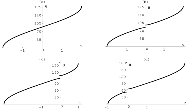
Figure 3: Values of the Young angle as functions of the celerity $u$ of the contact line. We plot different formal cases associated with relations $(16)_{1}$ and $(16)_{2}$ and convenient values of $\sigma_{10},\sigma_{2},k,\nu$. In panel (a), $k=0$ and the Young angle $\theta_{m}$ is $\displaystyle{\ 90^{\circ}}$. In panels (b), (c) and (d), $k\not=0$ and the Young angle $\displaystyle\theta_{m}$ has values $\displaystyle{90^{\circ}}$, $\displaystyle{120^{\circ}}$ or $\displaystyle{60^{\circ}}$. In cases (b), (c) and (d), we note a hysteresis phenemenon due to the discontinuity of $\theta$ for $u=0$. The unit of the u-axis depends on the fluids.

5 Comparison between results, experimental data and other models obtained in the literature

We propose a model of hysteresis of the contact system at the interface liquid-fluid-solid with the aid of which experimental results can be interpreted. Moreover, we find that the behaviour matches that obtained by kinetic molecular arguments in the literature.

5.1 The dynamic line tension behaviour

The differential equation (7) is equivalent to Eq. (3) in the form

$$\nu\,{\frac{dz}{dt}}=-\sigma_{2}\,\mathrm{cos}\,\theta\,-\sigma_{1}\ .$$

Following the expression for the solid-surface energy, the emerging equation admits a macroscopic behaviour expressed by the differential equation (12). When the piston is at rest, the macroscopic contact-line motion is governed by the equation (see Eq. (12)):

$$\nu\,{\frac{dz}{dt}}=\pm\,[(\sigma_{2}\,\mathrm{cos}\,\theta\,+\sigma_{10})^{2}-k^{2}\,\sigma_{10}^{2}]^{\frac{1}{2}}\ ,$$

where the sign $+$ or $-$ depends on the direction of the line motion and $k\,\sigma_{10}\equiv{\max\mid\sigma_{1}-\sigma_{10}\mid}$ is the maximum of the fluctuations in the fluid-solid energy with respect to its average value $\overline{\sigma}_{1}$.

The average value of the surface tension is $\tau=\sigma_{2}\,\mathrm{cos}\,\theta\,+\sigma_{10}$. It has the dimension of a force per unit length. If $\tau_{m}=-k\sigma_{10}$ represents the value of $\tau$ at $\theta=\theta_{A}(0)$ (see relation (14)), when the angle $\theta$ is close to $\theta_{A}(0)$, we obtain

$$\nu{\frac{dz}{dt}}=(\tau^{2}-\tau^{2}_{m})^{\frac{1}{2}}\approx\sqrt{2\,\tau_{m}}\,(\tau-\tau_{m})^{\frac{1}{2}}\ .$$

When the Young angles are small, on expanding $\theta$ to order 2, we obtain

$$\theta^{2}-\theta_{A}^{2}(0)\,\equiv\,\beta_{0}(\tau-\tau_{m})\ ,$$

where $\beta_{0}$ is a suitable constant.

The results are extendable to the case of a piston in advancing motion. Eq. (17) remains unchanged, but the dynamic angle of contact is such that

$$(\sigma_{2}\,\mathrm{cos}\,\theta\,+\sigma_{10})^{2}-k^{2}\sigma_{10}^{2}-\nu^{2}\,u^{2}=0\ .$$

Noting that $\displaystyle\tau_{u}=-\sqrt{(\sigma_{2}\,\mathrm{cos}\,\theta\,+\sigma_{10})^{2}-\nu^{2}\,u^{2}}$, the previous results are unchanged but $\mid\tau_{u}\mid<\mid\tau_{m}\mid$.

When the contact line retreats, it is easy to present similar calculations and to obtain analogous results.

These results are similar to those obtained in the literature by molecular statistics or single defects (Ruckenstein and Dunn, [26]). For example, Eq. (18) and Eq. (19) and an analysis of their consequences are also presented in Raphael and de Gennes, [25], Joanny and Robbins, [18].

5.2 Limit velocities of the contact line

Limit velocities for advancing and retreating contact lines have been experimentally found and described in detail (Hoffmann, [15], Dussan, [9], Blake and Ruschak, [4], Chen, Ramé and Garoff, [6], Decker et al, [8]). These velocities are generally outside the domain of validity of Eq. (3). Nevertheless, we formally extend our calculations to the case $\theta\in(0,\pi)$, and the asymptotic behaviour obtained in subsection 4.1 makes it possible to calculate the limit velocities! Of course, this extension corresponds to the fact that the forms of the graphs of $\theta$ as a function of $u$ presented in fig. 3 are similar to experimental graphs proposed in the literature. Indeed, the advancing Young angle must be smaller than $\pi$. The celerity of the contact line is $u_{\pi}$ and the associated line friction $\nu_{\pi}$. Relation $(16)_{1}$ yields

$$\nu_{\pi}\,u_{\pi}=\sqrt{(\sigma_{2}-\sigma_{10})^{2}-k^{2}\,\sigma_{10}^{2}}\ .$$

In the same way the retreating Young angle must be larger than $0$. The celerity of the contact line is now $u_{0}$ and the associated line friction $\nu_{0}$. Relation $(16)_{2}$ yields

$$\nu_{0}\,u_{0}=-\sqrt{(\sigma_{2}+\sigma_{10})^{2}-k^{2}\,\sigma_{10}^{2}}\ .$$

Notice that the velocities $u_{0}$ and $u_{\pi}$ do not have the same absolute value.
With this crude approximation, when the line friction is chosen with a constant value $\nu$, knowledge of $\sigma_{2}$, $\sigma_{10}=\overline{\sigma}_{1}$, $u_{0}$ and $u_{\pi}$ allows us to determine $K=k\,\sigma_{10}$ and $\nu$.

In the Appendix, it is proved that the representation (1) for the surface energy is only a convenient way to consider calculations with surface heterogeneities. The representation is extendable to any periodic function with variations on short intervals with respect to macroscopic sizes. Consequently, the previous results make it possible to investigate the surface quality and line friction by simple measurements.

5.3 Connection between the dynamic contact angle, the line celerity and the line friction

The purpose of this paragraph is to show by comparison with simple experiments that our model leads to qualitative and perhaps some quantitative coincidental behaviours of the contact system with experimental evidence. The simplest way is to consider the surface inhomogeneity given by our model represented by relation (1). The values of $\sigma_{10}$, $\sigma_{2}$ and $k$, allow us to draw the graphs of the applications given by $(16)_{1}$ and $(16)_{2}$, (see fig. 3). Only the ratio $\sigma_{10}/\sigma_{2}$ and the value of $k$ are important.

We present in fig. 4 experimental layouts drawn in the literature for an advancing motion of the contact line (Zhou and Sheng, [32]). The similarity of the theoretical graph and the experimental data is striking. Nevertheless, we must note that the experimental data in the literature is always presented in logarithmic scales. This comparison makes it possible to obtain numerical values for the line friction $\nu$ (as an average) and the limit velocities $u_{0}$ and $u_{\pi}$. We use the experimental results for liquid flows in contact with air in capillary tubes. Results do not take any explicit account of the inhomogeneity of the tube walls. In the model suggested by relation (1), the solid surface inhomogeneity is represented by the factor $k$. In fact, $k\ll 1$, and in relations (20) and (21) the term $k^{2}\,\sigma_{10}^{2}$ is neglected in comparison to the terms $(\sigma_{2}-\sigma_{10})^{2}$ and $(\sigma_{2}+\sigma_{10})^{2}$.

Figure 4: Apparent dynamic contact angle plotted as a function of $C_{a}=\mu_{0}\,{u/\sigma_{2}}$. The $C_{a}$-axis is based on a logarithmic scale. Panels (a) and (b) are associated with the data of J.P. Stokes et al. (ref. 13 from Zhou and Sheng, [32]). Panels (c) and (d) are associated with the data of G.M. Femigier and P. Jenffer (ref. 12 from Zhou and Sheng, [32]). Solid curves are calculated with $(16)_{1}$. The solid surfaces are assumed to be sufficiently smooth for the hysteresis to be small. It is easy to adjust the values of $\sigma_{10},\sigma_{2}$ and $\nu$ to fit the experimental data given by points.

In order to be in agreement with the experimental conditions, we suppose the diameter of the tube to be about $1$ mm. We deduce the numerical relations between the celerities $C_{a}$ and $u$ for two liquids. These expressions are given in c.g.s. units. For water we obtain $u=7200\,C_{a}\,$ and for glycerol $u=4.2\,C_{a}$. The experimental curves yield limit velocities of the contact line. In various measurements they represent values for $C_{a}$ and range between $10^{-2}$ and $10^{-1}$. For an air-glycerol interface, these values correspond to the limit celerity $u_{\pi}$ with a value between $0.042\,$ cm s ^-1 and $0.42\,$ cm s ^-1, and for an air-water interface the limit celerity $u_{\pi}$ lies between $72\,$ cm s ^-1 and $720\,$ cm s ^-1. They are widely out of the range of validity of our model, but for a wonder, they are in good agreement with experimental results!
For glycerol and a limit celerity of $0.42\,$ cm s ^-1 and for a static wetting angle $\theta_{A}(0)$ of about $50^{\circ}$, we obtain a line friction of about 240 Poise. For water and a limit celerity of $100\,$ cm s ^-1, the line friction is about one Poise. Let us note that the case of water is obviously less realistic than the case of glycerol. These values of the line friction are of the same order of magnitude as those obtained with relation (26) in part 1.

6 Conclusion

We proposed in this paper a dynamic model of slow movements of the contact system between two fluids and a solid surface. Comparison between our results and recent experiments or behaviour inferred from statistical physics shows good agreement on the qualitative level and, more unexpectedly, on the quantitative side. The most significant innovation in this paper is the introduction of the notion of line friction. This term is essential to the construction of the model. The line friction depends on the Young angle, but an order of magnitude for its average value can be obtained by using experimental measurements in the literature.

The Young-Dupré relation (3) takes the inhomogeneity on the solid surface into account. It describes the microscopic behaviour of the Young angle. The inhomogeneity is distributed at distances between a few tens to some hundred Angströms. This distance is that of the operating ranges of intermolecular forces which command the surface energies. At the lower part of this scale, energies are homogenized and these distances on a macroscopic scale are no longer significant. The shape of the surface is prescribed on larger scales.

The results are independent of the radius of the tube. Indeed, the hysteresis behaviour solely depends on the physico-chemical properties of the solid surface. The universal form of the hysteresis loop makes it possible to discuss the general case independently of any particular apparatus. Relations (20) and (21) can be written without difficulty using the inhomogeneity of the solid surface in a form different from Eq. (1).

Not all the efforts on the contact line have the same effects: the one associated with the rapid oscillations of the surface energy of the wall, ($K{\mathrm{s}in}\,(z/\varepsilon a)$), produces a work that tends to zero when the wave length of the oscillations tends to zero. This effort appears in the macroscopic expression of the contact line motion represented by Eq. (12). It is noteworthy that the weak differences between the potentials $W_{0}$ and $W_{e}$ have huge implications. This may seem surprising at first sight. It is due to the fact that the contact line is massless and consequently its motion equation is not in the same form as for material systems. Some authors model contact lines as lines with matter (Slattery, [27]); nevertheless, the inertial force associated with the mass of the line is generally of an order smaller than the magnitude of the force due to the line friction.

Finally we note that jumps on the inhomogeneity are considered by Jansons, [17]. A shift factor is proposed by Hoffman, [15], correcting the relation between $u$ and $\theta$. These considerations appear unnecessary in our model where movements are slow and $\theta$ is the apparent dynamic contact angle. Furthermore, the experimental literature notes the influence of evaporation on the relaxation time for approaching the apparent dynamic contact angle (Penn and Miller, [22]). Similar inferences are drawn for equipments which are subjected to vibrations (Marmur, [21]). The relaxation time of the apparent dynamic contact angle is obtained by phenomenological methods (Hoffman,[15], Penn and Miller, [22]). It corresponds to the calculations carried out in the Appendix.

Lastly, other models for high-speed motions of the contact line using a notion of dynamic surface energy are also considered in the literature: Shikhmurzaev, [28], Blake, Bracke and Shikhmurzaev, [5]. Their study is outside the scope of our slow movement model.

7 Appendix: Proof of the fundamental theorem

Consider the differential equation

$$\nu(z)\,{\frac{dz}{dt}}=f(z,t)\,+\,K\,sin\,{\frac{z}{\varepsilon}}\,$$

(we present the same differential equation as Eq. (7), but $f$ may be a more general function than listed in (7), and $a=1$ corresponds to the choice of a convenient unit of length).

The following hypotheses are assumed:

$\bullet\ K$ and $\varepsilon$ ($\varepsilon\ll 1$) are two strictly positive constants;

$\bullet\ f$ is continuously differentiable for any $z\in\Re$, and for any $t\in\Re^{+}$,

$\hskip 8.5359pt{\partial f}/{\partial z}<0$ ;

$\bullet\$There exist $z^{-}$ and $z^{+}$ belonging to $C^{1}(\Re)$ such that for any $t\in\Re^{+}$

$$f(z^{-},t)=K\,\,\,\,\mathrm{and}\,\,\,\,f(z^{+},t)=-K\,;$$

$\bullet\ \nu$ is a strictly positive continuous function of $z$.

Remarks: The fact that for $t$ fixed, $f(z,t)$ is a decreasing function on $[0,+\infty)$, implies $z^{-}<z^{+}$. Differential equation (A1) yields a single solution $z_{\varepsilon}(t)$ defined in $\Re^{+}$ with $z_{\varepsilon}(0)=z_{0}$, (the differentiable equation fulfills the conditions of uniqueness of the Cauchy problem (Hartman, [14])).

We obtain the fundamental result that gives the behaviour of $z_{\varepsilon}(t)$ when $\varepsilon$ tends to 0 from the following theorem

Asymptotic theorem

When $\varepsilon$ tends to $0$, $z_{\varepsilon}(t)$ converges uniformly to $z(t)$ belonging to $C^{1}[\Re^{+}]$ and satisfying the differential equation

$$\nu(z)\,{\frac{dz}{dt}}=g(z,t)\,,$$

where $z(0)=z_{0}$ and

$$g(z,t)=\left\{\begin{array}[]{ccl}\,\,[f^{2}-K^{2}]^{\frac{1}{2}}&\mathrm{if}&\;z<z^{-}(t)\,,\cr\cr 0&\mathrm{if}&\,\,z^{-}(t)<z<z^{+}(t)\,,\cr\cr\displaystyle-[f^{2}-K^{2}]^{\frac{1}{2}}&\mathrm{if}&\,\,\,z^{+}(t)<z\,.\end{array}\right.$$

The theorem, proved for $\nu(z)=$ constant, is extended without difficulty for $\nu(z)$ belonging to $[\alpha,\beta]$ where $0<\alpha<\beta<\infty\,\,$.

Let us give an elementary proof of the fundamental theorem. For a complete demonstration using Young measures, we refer to Abeyaratne, Chu and James, [1], [2]. We just consider the case $\nu=$ constant ($\nu=1$ with a convenient unit) and $f$ independent of $t$. For the variable $z$ belonging to a compact interval, the segment $[-1,1]$ is considered. The hypothesis ${\partial f}/{\partial z}<0$ corresponds to strict convexity of $W_{0}\,\Big{(}\partial W_{0}/{\partial z}=-f(z)\Big{)}$. For a given $\varepsilon$, consider $z_{0}\in[-1,1]$ as the initial value of the solution $z_{\varepsilon}(t)$ of Eq. (A1). The critical points of Eq. (A1) are the roots of

$$f(z)+K\,\mathrm{sin}\,{\frac{z}{\varepsilon}}=0\,.$$

The roots belong to the interval $[z^{-},z^{+}]$. Let us consider the case for which $z_{0}$ is smaller than $z^{-}$; when $\,T\,$ is sufficiently small, it is the same for $z_{\varepsilon}(t)$ with $t\in[0,T]$. Let us calculate the limit values $t$ according to position $z$ when $\varepsilon$ tends to zero. For $\varepsilon\ll 1$, the function $\,\mathrm{sin}\,({{z}/{\varepsilon}})$ oscillates rapidly between -1 and 1. Let $z_{0,\varepsilon}$ be the value immediately above or equal to $z_{0}$ such that $\,\mathrm{sin}\,({{z_{0,\varepsilon}}/{\varepsilon}})=-1$ and let $z_{1,\varepsilon}$ be the value immediately below or equal to $z_{\varepsilon}(t)$ such that $\,\mathrm{sin}\,({{z_{1,\varepsilon}}/{\varepsilon}})=1$. Then,

$$\lim_{\varepsilon\rightarrow\,0\,\,}\int_{z_{0,\varepsilon}}^{z_{1,\varepsilon}}{\frac{dz}{{f(z)+K\mathrm{sin}\displaystyle{\frac{z}{\varepsilon}}}}}=t\,.$$

Let us divide the interval $[z_{0,\varepsilon},z_{1,\varepsilon}]$ in intervals of length $\varepsilon\pi$. Then,

$$\int_{z_{0,\varepsilon}}^{z_{1,\varepsilon}}{\frac{dz}{{f(z)+K\mathrm{sin}\displaystyle{\frac{z}{\varepsilon}}}}}=\sum_{p=0}^{N-1}\int_{z_{0,\varepsilon}+p\varepsilon\pi}^{z_{0,\varepsilon}+(p+1)\varepsilon\pi}{\frac{dz}{{f(z)+K\mathrm{sin}\displaystyle{\frac{z}{\varepsilon}}}}}\ ,$$

where $N=(z_{1,\varepsilon}-z_{0,\varepsilon})/(\varepsilon\pi)$

At each interval $\,[{z_{0,\varepsilon}+p\varepsilon\pi},{z_{0,\varepsilon}+(p+1)\varepsilon\pi}]\,$ the change of variables $\,s=\mathrm{sin}\,\displaystyle{\frac{z}{\varepsilon}}\,$ yields

$$\int_{z_{0,\varepsilon}}^{z_{1,\varepsilon}}{\frac{dz}{{f(z)+K\mathrm{sin}\displaystyle{\frac{z}{\varepsilon}}}}}=\sum_{p=0}^{N-1}\int_{-1}^{+1}{\frac{\varepsilon\,ds}{{(f(\lambda)+Ks)\sqrt{1-s^{2}}}}}\ ,$$

where $\lambda=\varepsilon\,\mathrm{arcsin}\,s$ and $\lambda\in\displaystyle{[\varepsilon p\pi-\varepsilon{\frac{\pi}{2}},\varepsilon p\pi+\varepsilon{\frac{\pi}{2}}]}$. Because $f$ is continuous, this expression has the same limit when $\varepsilon$ tends to zero as

$${\frac{1}{\pi}}\sum_{p=0}^{N-1}\varepsilon\pi\int_{-1}^{+1}{\frac{ds}{{(f(\varepsilon p\pi-\varepsilon{\frac{\pi}{2}})+Ks)\sqrt{1-s^{2}}}}}$$

or

$${\frac{1}{\pi}}\sum_{p=0}^{N-1}\varepsilon\pi\int_{-1}^{+1}{\frac{ds}{{(f(\varepsilon p\pi+\varepsilon{\frac{\pi}{2}})+Ks)\sqrt{1-s^{2}}}}}\ ,$$

which are two sums of Darboux integrals

$${\ \int_{z_{0,\varepsilon}}^{z_{1,\varepsilon}}{\frac{1}{\pi}}\left(\int_{-1}^{+1}{\frac{ds}{{(f(z)+Ks)\sqrt{1-s^{2}}}}}\right)\,dz}\,.$$

When $\varepsilon$ tends to zero, this expression converges to

$$\int_{z_{0}}^{z(t)}{\frac{1}{\pi}}\left(\int_{-1}^{+1}{\frac{ds}{{(f(z)+Ks)\sqrt{1-s^{2}}}}}\right)\,dz=t\,.$$

Because $f(z)^{2}\geq K^{2}$, the change of variables $\,s=\mathrm{sin}\,\alpha\,$ yields

$$\int_{-1}^{+1}{\frac{ds}{{(f(z)+Ks)\sqrt{1-s^{2}}}}}={\frac{\pi}{\sqrt{f(z)^{2}-K^{2}}}}$$

and finally,

$$\int_{z_{0}}^{z(t)}{\frac{dz}{\sqrt{f(z)^{2}-K^{2}}}}=t\ ,$$

which implies

$$\dot{z}=\sqrt{f(z)^{2}-K^{2}}\ .$$

In the same way, for $z_{0}$ above $z^{+}$ we obtain,

$$\dot{z}=-\sqrt{f(z)^{2}-K^{2}}\ .$$

When $z_{0}$ belongs to the interval $[z^{-},z^{+}]$, it is easily seen that there exists a critical point$\;\overline{z_{\varepsilon}}$ of Eq. (A1) such that $\mid\overline{z_{\varepsilon}}-z_{0}\mid<b\,\varepsilon$ where $\,b\,$ is a positive constant depending only on $K$ and $f$. The solution of Eq. (A1) tends in a monotonous way towards $\overline{z_{\varepsilon}}$. Consequently, for $t$ belonging to $[0,+\infty[$, $z_{\varepsilon}(t)$ converges uniformly to $z_{0}$ when $\varepsilon$ tends to zero. The macroscopic law associated to $z_{0}$ belonging to $[z^{-},z^{+}]$ is $\dot{z}=0$.

General oscillations

We consider the superimposed effect of an arbitrary smooth periodic function $\displaystyle P({{z}/{\varepsilon}})$ in place of $\mathrm{sin}\,({{z}/{\varepsilon}})$. We can assume without loss of generality that $\displaystyle P({{z}/{\varepsilon}})$ has a zero average, (in other cases, we add a constant to $f$).

The amplitude of $P$ gives the placement of the flat region as in figure 2:

$$-\mathrm{max}\,P\,\leq\,f(z,t)\,\leq\,-\mathrm{min}\,P$$

With the same hypotheses as in the theorem we define $z^{-}(t)$ and $z^{+}(t)$ such that

$$f(z^{-}(t),t)=-\mathrm{min}\,P\,\,\,\,\mathrm{and}\,\,\,\,f(z^{+}(t),t)=-\mathrm{max}\,P\ ;$$

so the flat region remains $[z^{-}(t),z^{+}(t)]$.

In the special case when $f$ is independent of $t$, the calculation is developed in the same way as previously. The results are unaltered with $-\mathrm{min}\,P$ in place of $K$ and $-\mathrm{max}\,P$ in place of $-K$.

The complete proof of this extension is given in Abeyaratne, Chu and James, [2].

Relaxation time associated with Eq. (A3)

We consider the case when $g$ is explicitly independent of $t$ and $\nu$ is constant. For $z_{0}<z^{-}$, let

$$\chi=\nu\,\int_{z_{0}}^{z^{-}}\,{\frac{du}{\sqrt{f(u)^{2}-K^{2}}}}\ .$$

For $z_{0}$ near $z^{-}$, $f(u)+K\sim 2\,K$ and $f(u)-K\sim(u-z^{-})f^{\prime}(z^{-})$. Then, $f(u)^{2}-K^{2}\sim 2\,K(u-z^{-})f^{\prime}(z^{-})$ and

$$\chi\,\sim\,\nu\,\sqrt{\frac{2}{{-K\,f^{\prime}(z^{-})}}}\,\sqrt{z^{-}-z_{0}}\ .$$

The $\chi$-value yields the magnitude of the relaxation time necessary to obtain the final position of the contact line.

References

- [1] Abeyaratne R, Chu C, James RD (1994) Proceedings of the Symposium on the Mechanics of Phase Transformations and Shape Memory alloys, Applied Mechanics Division, American Society of Mechanical Engineers, New-York, 109 pp 85-98
- [2] Abeyaratne R, Chu C, James RD (1996) Kinetics of materials with wiggly energies: theory and application to the evolution of twinning microstructures in a Cu-Al-Ni shape memory alloy. Philosophical Magazine A 73: 457-497
- [3] Baiocci C, Pukhnachev VV (1990) Problems with one-sided constraints for Navier-Stokes equations and the dynamic contact angle. Journal of applied mechanics and technical physics (translated from russian) 31: 185-197
- [4] Blake TD, Ruschak KJ (1979) A maximum speed of wetting. Nature 282: 489-491
- [5] Blake TD, Bracke M, Shikhmurzaev YD (1999) Experimental evidence of nonlocal hydrodynamic influence on the dynamic contact angle. Physics of Fluids 11: 1995-2007
- [6] Chen Q, Ramé E, Garoff S (1997) The velocity field near moving contact line. J. Fluid Mech. 337: 49-66
- [7] Concus P. (1968) Static menisci in a vertical right cylinder. J. Fluid Mech. 34: 481-495
- [8] Decker EL, Frank B, Suo Y, Garoff S (1999) Physics of contact angle measurement. Colloid and Surfaces A 156: 177-189
- [9] Dussan V EB (1979) On the spreading of liquids on solid surfaces: static and dynamic contact-lines. Annual Rev. Fluid Mech. 11: 371-400
- [10] Dussan V EB, Ramé E, Garoff S (1991) On identifying the appropriate boundary conditions at a moving contact-line: an experimental investigation. J. Fluid Mech. 230: 97-116
- [11] Finlow DE, Kota PR, Bose A (1996) Investigations of wetting hydrodynamics using numerical simulations. Phys. Fluids 8: 302-309
- [12] Foister RT (1990) The kinetics of displacement wetting in liquid/liquid/solid systems. J. Colloid Interface Sci 136: 266-282
- [13] Gouin H (2003) The wetting problem of fluids on solid surfaces. Part 1: the dynamics of contact lines. Cont Mech. and Therm. In press
- [14] Hartman P (1990) Ordinary differential equations. John Wiley, New York
- [15] Hoffman R (1975) A study of the advancing interface. Interface-shape in liquid-gas systems. J. Colloid Interface Sci. 50: 228-241
- [16] Huh C, Mason SG (1977) Effects of surface roughness on wetting (theoritical). J. Colloid Interface Sci. 60: 11-38
- [17] Jansons KM (1986) Moving contact lines at a non-zero capillary number. J. Fluid Mech. 167: 393-407
- [18] Joanny JF, Robbins MO (1990) Motion of a contact line on a heterogeneous surface. J. Chem. Phys. 92: 3206-3212
- [19] Legait B, Sourieau P (1985) Effects of geometry on a advancing contact angle in fine capillaries. J. Colloid Interface Sci. 107: 14-20
- [20] Lowndes J (1980) The numerical simulation of the steady movement of a fluid meniscus in a capillary tube. J. Fluid Mech. 101: 631-646
- [21] Marmur A (1996) Equilibrium contact angles: theory and measurement. Colloid and Surfaces A 116: 55-61
- [22] Penn LS, Miller B (1980) A study of primary cause of contact angle hysteresis on some polymeric solids. J. Colloid Interface Sci. 78: 238-241
- [23] V.V. Pukhnachev (1989) Thermocapillary convection under low gravity. Fluid Dynam. Trans. 14 Warsaw
- [24] Ramé E, Garoff S (1996) Microscopic and macroscopic dynamic interface shapes and the interpretation of dynamic contact angles. J. Colloid Interface Sci. 177: 234-244
- [25] Raphael E, de Gennes PG (1989) Dynamics of wetting with nonideal surfaces. The single defect problem. J. Phys. Chem. 90: 7577-7584
- [26] Ruckenstein E, Dunn CS (1977) Slip velocity during wetting of solids. J. Colloid Interface Sci. 59: 135-138
- [27] Slattery JC (1990) Interfacial transport phenomena. Springer-Verlag, Berlin
- [28] Shikhmurzaev YD (1997) Moving contact lines in liquid/liquid/solid systems. J. Fluid Mech. 334: 211-249
- [29] Thompson PA, Robbins MO (1990) To slip or not to slip, Phys. World 3, 11: 35-38
- [30] Voinov OV (1995) Motion of line of contact of three-phases on a solid: thermodynamics and asymptotic theory. Int. J. Multiphase Flow 21: 801-816
- [31] West GD (1911) On the resistance to the motion of a thread of mercury in a glass tube. Proc. Roy. Soc. A 86: 20-24
- [32] Zhou MY, Sheng P (1990) Dynamics of immiscible fluid displacement in a capillary. Phys. Rev. Letter 64: 882-885