Strong and weak coupling limits in optics of quantum well excitons

Abstract

A transition between the strong (coherent) and weak (incoherent) coupling limits of resonant interaction between quantum well (QW) excitons and bulk photons is analyzed and quantified as a function of the incoherent damping rate $\gamma_{\rm x}$ caused by exciton-phonon and exciton-exciton scattering. For confined QW polaritons, a second, anomalous, $\gamma_{\rm x}$-induced dispersion branch arises and develops with increasing $\gamma_{\rm x}$. In this case, the strong-weak coupling transition is attributed to $\gamma_{\rm x}=\gamma_{\rm x}^{\rm tr}$ or $\tilde{\gamma}_{\rm x}^{\rm tr}$, when the intersection of the normal and damping-induced dispersion branches occurs either in $\{k_{\|},\mbox{Im}[\omega],\mbox{Re}[\omega]\}$ coordinate space (in-plane wavevector $k_{\parallel}$ is real) or in $\{\omega,\mbox{Im}[k_{\parallel}],\mbox{Re}[k_{\parallel}]\}$ coordinate space (frequency $\omega$ is real), respectively. For the radiative states of QW excitons, i.e., for radiative QW polaritons, the transition is described as a qualitative change of the photoluminescence spectrum at grazing angles along the QW structure. We show that the radiative corrections to the QW exciton states with in-plane wavevector $k_{\parallel}$ approaching the photon cone, i.e., at $k_{\parallel}\rightarrow k_{0}\!=\!(\omega_{0}\sqrt{\varepsilon_{\rm{b}}})/(\hbar c)$ ($\varepsilon_{\rm{b}}$ is the background dielectric constant), are universally scaled by the energy parameter $\big{(}\Gamma_{0}^{2}\omega_{0}\big{)}^{1/3}$ with $\Gamma_{0}$ the intrinsic radiative width and $\omega_{0}$ the exciton energy at $k_{\parallel}=0$, rather than diverge. Similarly, the strong-weak coupling transition rates $\gamma_{\rm x}^{\rm tr}$ and $\tilde{\gamma}_{\rm x}^{\rm tr}$ are also proportional to $\big{(}\Gamma_{0}^{2}\omega_{0}\big{)}^{1/3}$. The numerical evaluations are given for a GaAs single quantum well with realistic parameters: $\Gamma_{0}=45.5\,\mu$eV and $\big{(}\Gamma_{0}^{2}\omega_{0}\big{)}^{1/3}\approx 1.5$ meV.

I INTRODUCTION

Since the pioneering work by Agranovich and Dubovskii Agranovich , optics of quasi-two-dimensional (quasi-2D) QW excitons became a well-established discipline. Traditionally, the states of optically-dressed QW excitons are classified in terms of confined quantum well polaritons (or simply QW polaritons) and radiative quantum well polaritons (or simply the radiative states of QW excitons). The QW polaritons are trapped and in-plane guided by the exciton resonance, accompanied by an evanescent light field in the growth direction (the $z$-direction), and characterized by a single dispersion branch $\omega=\omega(k_{\parallel})$ which lies outside the photon cone $\omega=(\hbar ck)/\sqrt{\varepsilon_{\rm{b}}}$ in the $\{k_{\parallel},\omega\}$ plane Nakayama ; Nakayama0 ; Andreanib ; Andreania ; Jorda1 ; Ivchenko91 . Although QW polaritons are invisible in standard, far-field, experiments, they can considerably contribute to the total optical response associated with QW excitons in a “hidden” way (see, e.g., Refs. [Ivanov97, ; Ivanov98, ; Ivanov04, ]). The radiative states of QW excitons, which refer to the radiative zone $k_{\parallel}\leq k_{0}$, can optically decay into bulk photon modes and therefore are characterized by a finite radiative lifetime Orrit ; Hanamura ; Andreanic ; Citrin1 . The radiative states of QW excitons have been observed and studied in many far-field optical, both photoluminescence (PL) and scattering (reflectivity/transmissivity), experiments (see, e.g., Refs. [Feldmann, ; Deveaud1, ; Gurioli, ; Eccleston, ; Martinez, ; Vinattieri, ; Szczytko, ; Deveaud2, ; Moret, ]). In turn, confined QW polaritons can be detected by using periodic grating Kohl and attenuated total reflection Lagois techniques, as well as with near-field scanning optical microscopy Hess and PL imaging spectroscopy Wu ; Pulizzi .

For GaAs QWs, confined and radiative QW polaritons are usually described in terms of $X-$, $Y-$ and $Z-$modes Nakayama ; Nakayama0 ; Hanamura ; Andreanic ; Andreanib . The $X-$mode states are in-plane longitudinal with polarization along ${\textbf{{k}}}_{\|}$, the $Y-$mode states are in-plane transverse with polarization normal to ${\textbf{{k}}}_{\|}$, and the $Z-$mode states are transverse with polarization along the $z$-axis. Thus the $Y-$mode ($X-$ and $Z-$mode) states couple with the $s$-polarized ($p$-polarized) light field. The $Z-$mode is absent for confined and radiative QW polaritons associated with the heavy-hole exciton state in a GaAs quantum well Andreanic ; Andreanib .

The main aim of the present work is to study how the resonant coupling between quantum well excitons and bulk photons relaxes with increasing homogeneous width $\gamma_{\rm x}$, due to incoherent scattering of QW excitons. In particular, in order to quantify the strong-weak coupling transition, we apply an approach developed in Refs. [Tait, ; Quattropani, ] for bulk polaritons: The transition is attributed to the intersection of the polariton dispersion branches that results in the topological change “crossing” $\leftrightarrow$ “anti-crossing” in the dispersion branches, in either $\{k_{\|},\mbox{Im}[\omega],\mbox{Re}[\omega]\}$ or $\{\omega,\mbox{Im}[k_{\parallel}],\mbox{Re}[k_{\parallel}]\}$ three-dimensional (3D) spaces (a similar paradigm has been used for quasi-zero-dimensional polaritons in semiconductor photonic dots Nikolaev ). The first quasi-particle case, when the in-plane wavevector $k_{\parallel}$ is real, refers to a PL experiment, while the second forced-harmonic case, when the frequency $\omega$ is real, can be applied to describe a scattering (reflectivity/transmissivity) experiment. In this paper we analyze the $\gamma_{\rm x}$-induced change of $Y-$mode QW polaritons, which are akin to transverse bulk polaritons. Note that neither the orthogonality between the $X-$, $Y-$ and $Z-$modes nor the orthogonality between the radiative and confined polariton states of the same mode is violated in the presence of the incoherent scattering rate $\gamma_{\rm x}$, at least within the mean-field picture we use in our study.

In contrast with bulk exciton-polaritons whose two dispersion branches exist for any value of $\gamma_{\rm x}$ and are given by two solutions of the bi-quadratic dispersion equation Hopfield ; Agranovich0 ; Tait ; Quattropani , the dispersion equation of $Y-$mode ($s$-polarized) QW polaritons can straightforwardly be reduced to a bi-cubic equation. As a result, a second anomalous damping-induced dispersion branch of confined quantum well polaritons arises and develops with increasing $\gamma_{\rm x}$. The existence of the additional $\gamma_{\rm x}$-induced dispersion branch is natural and allows us to attribute the strong-weak coupling transition to the intersection between the normal and anomalous dispersion branches. As we clarify in this work, the intersection points refer to $k_{\parallel}=k_{\|}^{\rm tr}=k_{0}-[(3\sqrt{\varepsilon_{\rm{b}}})/(2\sqrt[3]{4}\,\hbar c)]\big{(}\Gamma_{0}^{2}\omega_{0}\big{)}^{1/3}\simeq k_{0}$ for the quasi-particle case and to $\omega=\omega^{\rm tr}=\omega_{0}+(\omega_{0}^{2}\varepsilon_{\rm{b}})/(2c^{2}M_{\rm x})-[3/(4\sqrt[3]{4})]\big{[}(\omega_{0}\varepsilon_{\rm{b}})/(M_{\rm x}c^{2})\big{]}^{1/3}\big{(}\Gamma_{0}^{2}\omega_{0}\big{)}^{1/3}\simeq\omega_{0}$ for the forced-harmonic case, and the transition (threshold) damping rates are given by $\gamma_{\rm x}^{\rm tr}=[(3\sqrt{3})/(2\sqrt[3]{4})]\big{(}\Gamma_{0}^{2}\omega_{0}\big{)}^{1/3}$ and ${\tilde{\gamma}}_{\rm x}^{\rm tr}=[(3\sqrt{3})/2]\big{[}(\omega_{0}\varepsilon_{\rm{b}})/(M_{\rm x}c^{2})\big{]}^{1/3}\big{(}\Gamma_{0}^{2}\omega_{0}\big{)}^{1/3}$ ($M_{\rm x}$ is the in-plane translational mass of a QW exciton), respectively. The above analytic expressions are surprisingly simple, taking into account a rather non-trivial analysis of the two-fold degeneracy of complex roots of the bi-cubic dispersion equation we have developed in order to find $\gamma_{\rm x}^{\rm tr}$ and ${\tilde{\gamma}}_{\rm x}^{\rm tr}$ (similar expressions for bulk polaritons can be obtained in a much more straightforward way, as detailed in Refs. [Tait, ; Quattropani, ]).

For radiative $Y-$mode polaritons, i.e., for the radiative states of QW excitons, which are described in terms of their radiative width $\Gamma=\Gamma_{\rm T}(k_{\parallel})$ and (Lamb) shift $\Delta=\Delta_{\rm T}(k_{\parallel})$, we show that the radiative width $\Gamma_{\rm T}$ does not diverges at $k_{\parallel}=k_{0}$ even for the completely coherent interaction between QW excitons and bulk photons, when $\gamma_{\rm x}=0$. While the latter conclusion contradicts the known result of perturbation theory Hanamura ; Andreanic ; Citrin1 , i.e., that $\Gamma_{\rm T}$ diverges as $\Gamma_{\rm T}\propto 1/(k_{0}^{2}-k_{\parallel}^{2})^{1/2}$ when $k_{\parallel}\rightarrow k_{0}$, it is consisted with numerical simulations reported in the earlier studies Orrit ; Jorda2 ; Popov . We prove the regularization of the radiative corrections at $k_{\parallel}=k_{0}$ and show that both $\Gamma_{\rm T}(k_{\parallel}\!=\!k_{0})$ and $\Delta_{\rm T}(k_{\parallel}\!=\!k_{0})$ are universally scaled by $\big{(}\Gamma_{0}^{2}\omega_{0}\big{)}^{1/3}$. There is no extra dispersion branch, induced by damping, relevant to the radiative states of QW excitons. However, the strong-weak coupling transition can still be seen as a $\gamma_{\rm x}$-induced qualitative change of the radiative corrections at $k_{\parallel}\simeq k_{0}$ and can be observed in photoluminescence at grazing angles along the QW structure. The transition occurs synchronously for both radiative and confined QW polaritons.

Thus the main results of the work are (i) regularization of the radiative corrections to the QW exciton states at $k_{\parallel}\rightarrow k_{0}$, with the energy parameter $\big{(}\Gamma_{0}^{2}\omega_{0}\big{)}^{1/3}$, (ii) the $\gamma_{\rm x}$-induced anomalous dispersion branch of QW polaritons, and (iii) a quantitative description of the strong-weak coupling transition for resonant interaction of bulk photons and QW excitons in the presence of incoherent scattering. Our numerical simulations refer to a realistic high-quality GaAs single quantum well of the width $d_{z}=25$ nm [Ivanov04, ].

In Sec. II, a Hamiltonian relevant to resonantly interacting QW excitons and bulk photons is outlined, and the dispersion equation is derived by using diagram technique in order to include the incoherent scattering rate $\gamma_{\rm x}$.

In Sec. III, for the case of completely coherent interaction between QW excitons and bulk photons (the strong coupling limit, $\gamma_{\rm x}=0$), we discuss the regularization of the radiative corrections to the QW exciton states at $k_{\parallel}\simeq k_{0}$ and quantify characteristic points $A$ ($k_{\parallel}=k_{0}$) and $B$ ($k_{\parallel}=k_{\|}^{\rm(B)}>k_{0}$). It is shown that for point $A$ the radiative width $\Gamma_{\rm T}$ reaches its maximum value $\Gamma_{\rm T}^{\rm(A)}\propto\big{(}\Gamma_{0}^{2}\omega_{0}\big{)}^{1/3}$, while for the terminal point $B$ the Lamb shift $\Delta_{\rm T}$ of the QW radiative states has a maximum value $\Delta_{\rm T}\propto\big{(}\Gamma_{0}^{2}\omega_{0}\big{)}^{1/3}$.

In Sec. IV, we analyze the QW polariton states in the presence of incoherent scattering and, in particular, prove that the second, anomalous, QW polariton dispersion branch exists for $\gamma_{\rm x}\geqslant\gamma_{\rm c}^{(1)}=\Gamma_{0}$. It is shown that the optical brightness, i.e., the visibility, of the second dispersion branch drastically increases when the in-plane wavevector $k_{\parallel}$ approaches $k_{0}$. We also quantify the threshold damping rates, $\gamma_{\rm x}^{\rm tr}$ (quasi-particle solutions) and $\tilde{\gamma}_{\rm x}^{\rm tr}$ (forced-harmonic solutions), when the strong-weak coupling transition occurs, and demonstrate that both $\gamma_{\rm x}^{\rm tr}$ and $\tilde{\gamma}_{\rm x}^{\rm tr}$ are scaled by the energy parameter $\big{(}\Gamma_{0}^{2}\omega_{0}\big{)}^{1/3}$.

In Sec. V, the transition between the strong and weak coupling limits is analyzed for the radiative states of QW excitons. We show that the $\gamma_{\rm x}$-induced radiative states can persist far beyond the terminal point $B$, i.e., at $k_{\parallel}>k_{\|}^{\rm(B)}$, and that with increasing $\gamma_{\rm x}$ across $\gamma_{\rm x}^{\rm tr}$ the radiative corrections drastically change their shape, $\Gamma_{\rm T}=\Gamma_{\rm T}(k_{\parallel})$ and $\Delta_{\rm T}=\Delta_{\rm T}(k_{\parallel})$, in the vicinity of $k_{\parallel}=k_{0}$.

In Sec. VI, we discuss how damping-induced QW polaritons of the anomalous dispersion branch and the strong-weak coupling transition can be detected by using near-field optical spectroscopy. It is also shown that the $\gamma_{\rm x}$-induced change of the PL signal from the QW exciton radiative states at $k_{\parallel}\simeq k_{0}$ (photoluminescence at grazing angles) allows to visualize the strong-weak coupling transition.

A short summary of the results is given in Sec. VII.

II MODEL

The Hamiltonian of a system “bulk photons – QW excitons”, in the presence of dipole interaction between two species, is given by

$$H=H_{\gamma}+H_{\rm x}+H_{i}^{\rm I}+H_{i}^{\rm II}\,,$$ (1)

with

$$H_{\gamma} = \sum_{\textbf{{k}}}\omega^{\gamma}_{\textbf{{k}}}\alpha^{{\dagger}}_{\textbf{{k}}}\alpha_{\textbf{{k}}}\,,\ \ \ \ \ H_{\rm x}=\sum_{\textbf{{k}}_{\parallel}}\omega^{\rm x}_{\textbf{{k}}_{\parallel}}b^{{\dagger}}_{\textbf{{k}}_{\parallel}}b_{\textbf{{k}}_{\parallel}}\,,$$

$$H_{i}^{\rm I} = i\sum_{\textbf{{k}}_{\parallel}}\sum_{k_{z}}(\omega^{\rm x}_{\textbf{{k}}_{\parallel}})^{1/2}C_{\textbf{{k}}_{\parallel},k_{z}}(\alpha_{\textbf{{k}}_{\parallel},k_{z}}+\alpha^{\dagger}_{-\textbf{{k}}_{\parallel},-k_{z}})(b_{-\textbf{{k}}_{\parallel}}-b^{\dagger}_{\textbf{{k}}_{\parallel}})\,,$$

$$H_{i}^{\rm II} = \sum_{\textbf{{k}}_{\parallel}}\sum_{k_{z},k^{{}^{\prime}}_{z}}C_{\textbf{{k}}_{\parallel},k_{z}}C_{\textbf{{k}}_{\parallel},k^{{}^{\prime}}_{z}}(\alpha_{\textbf{{k}}_{\parallel},k_{z}}+\alpha^{\dagger}_{-\textbf{{k}}_{\parallel},-k_{z}})(\alpha_{-\textbf{{k}}_{\parallel},-k^{{}^{\prime}}_{z}}+\alpha^{\dagger}_{\textbf{{k}}_{\parallel},k^{{}^{\prime}}_{z}})\,,$$ (2)

where $b_{\textbf{{k}}_{\parallel}}$ and $\alpha_{\textbf{{k}}}$ are the QW exciton and bulk photon operators, respectively, $\omega^{\rm x}_{\textbf{{k}}_{\parallel}}=\omega_{0}+(\hbar^{2}k_{\parallel}^{2})/(2M_{\rm x})$ and $\omega^{\gamma}_{\textbf{{k}}}=(\hbar c\textit{k})/\sqrt{\varepsilon_{\rm b}}$ are the exciton and photon dispersions, respectively. The coupling constant $C_{\textbf{{k}}_{\parallel},k_{z}}$ is given by $C_{\textbf{{k}}_{\parallel},k_{z}}=[R_{\rm QW}/(2{\omega^{\gamma}_{\textbf{{k}}}L})]^{1/2}$, where $R_{\rm QW}$ is the dimensional oscillator strength of exciton-photon interaction per QW unit area and $L$ is the $z$-direction quantization length of the light field ($L\rightarrow\infty$). The Hamiltonian (1) is relevant to the optics of transverse QW excitons which interact with the in-plane TE-polarized light field ($Y$-mode). The photon-mediated long-range exchange interaction and non-resonant terms of QW exciton – bulk photon coupling are included in the description.

The quadratic Hamiltonian (1) is exactly solvable, giving rise to the quasi-2D polariton and radiative states of QW excitons. This case deals only with coherent interaction between the particles [$H_{i}^{\rm I}$ and $H_{i}^{\rm II}$ terms in Eqs. (1)-(2)] and therefore inherently refers to the strong coupling between QW excitons and bulk photons. Alternatively, the (quasi-) eigen-energies of QW excitons can be found from Eq. (1) by using standard diagram technique [Hanamura, ; Citrin1, ; Jorda1, ; Jorda2, ]. The latter approach allows us to include the particle rate $\gamma_{\rm x}$ of incoherent scattering of QW exciton, i.e., the homogeneous broadening. The Dyson equation for QW excitons is

$$G_{\textbf{{k}}_{\parallel}}(\omega)=G_{\textbf{{k}}_{\parallel}}^{(0)}(\omega)+G_{\textbf{{k}}_{\parallel}}^{(0)}(\omega)\Sigma_{\textbf{{k}}_{\parallel}}(\omega)G_{\textbf{{k}}_{\parallel}}(\omega)\,,$$ (3)

where $G_{\textbf{{k}}_{\parallel}}^{(0)}=2\omega_{\textbf{{k}}_{\parallel}}^{\rm x}/[\omega^{2}-(\omega_{\textbf{{k}}_{\parallel}}^{\rm x}-i\gamma_{\rm x}/2)^{2}]$ and $G_{\textbf{{k}}_{\parallel}}$ are the propagators of optically-non-interacting and optically-dressed excitons, respectively, and the photon-mediated self-energy is given by

$$\Sigma_{\textbf{{k}}_{\parallel}}(\omega)=\frac{2\omega^{2}}{\omega_{\textbf{{k}}_{\parallel}}^{\rm x}}\sum_{k_{z}}\frac{\mid C_{\textbf{{k}}_{\parallel},k_{z}}\mid^{2}\omega^{\gamma}_{\textbf{{k}}}}{\omega^{2}-(\omega^{\gamma}_{\textbf{{k}}})^{2}}\,.$$ (4)

Straightforward calculation of the poles of $G_{\textbf{{k}}_{\parallel}}(\omega)=2\omega_{\textbf{{k}}_{\parallel}}^{\rm x}/[\omega^{2}-(\omega_{\textbf{{k}}_{\parallel}}^{\rm x}-i\gamma_{\rm x}/2)^{2}-2\omega_{\textbf{{k}}_{\parallel}}^{\rm x}\Sigma_{\textbf{{k}}_{\parallel}}(\omega)]$, which is obtained from Eqs. (3)-(4), yields the spectrum of optically-dressed QW excitons:

$$\omega^{2}-(\omega_{\textbf{{k}}_{\parallel}}^{\rm x}-i\gamma_{\rm x}/2)^{2}+\frac{\varepsilon_{\rm b}R_{\rm QW}\omega^{2}}{c^{2}\hbar^{2}\sqrt{k_{\parallel}^{2}-k^{2}(\omega)}}=0\,,$$ (5)

where $k(\omega)=(\omega\sqrt{\varepsilon_{\rm{b}}})/(\hbar c)$. For $\gamma_{\rm x}=0$, when no decoherence of exciton-photon interaction occurs, the dispersion Eq. (5) can also be derived by solving the Hamiltonian (1).

Both the confined and radiative states are nonperturbatively described by the same Eq. (5), the fact not completely realized in literature. The QW polariton, confined modes, which are characterized by $\mbox{\rm Im}[\omega]\leq 0$ and $\mbox{\rm Re}[\kappa]>0$ with $\kappa=\sqrt{k_{\|}^{2}-k^{2}(\omega)}$, refer to the physical sheet of the two-fold Riemann energy plane, while the radiative polariton modes with $\mbox{\rm Im}[\omega]\leq 0$ and $\mbox{\rm Re}[\kappa]<0$ are located on the unphysical sheet of the energy plane. The latter result is a signature of the metastable states decaying in outgoing waves [Landau, ]. Thus in order to find the energy spectrum of the radiative states, one has to use $-\kappa$ with $\mbox{\rm Re}[\kappa]>0$ for $\sqrt{k_{\|}^{2}-k^{2}(\omega)}$ in Eq. (5). This can also be justified by analyzing Eq. (3) for the radiative states in terms of the advanced, rather than retarded, Green functions. The initial three-dimensional Hamiltonian (1) maps on to a non-Hermitian two-dimensional Hamiltonian which has the quasi-spectrum given by Eq. (5) and describes the localized states (confined polaritons), which are split-off from the continuum, and the metastable states (radiative polaritons).

The dispersion Eq. (5) for $Y$-mode QW polaritons was widely discussed in the last two decades for the case $\gamma_{\rm x}=0$ [Nakayama, ; Nakayama0, ; Andreanib, ; Jorda1, ; Jorda2, ]. In contrast, the radiative states of QW excitons were mainly considered in terms of perturbation theory [Hanamura, ; Andreanic, ; Citrin1, ]. Equation (5) allows us to treat the radiative states non-perturbatively, what is particularly important for the vicinity of the resonant crossover between the dispersions of bulk photons and QW excitons, i.e., when $k_{\|}\rightarrow k_{0}=k(\omega_{0})$. While the main aim of the present paper is to study how the confined and radiative states depend on the incoherent damping rate $\gamma_{\rm x}$, in the following Section we detail a nonperturbative analysis of the radiative states by solving Eq. (5) for $\gamma_{\rm x}=0$.

III Non-perturbative radiative corrections to the exciton states in quantum wells

The radiative half-width $\Gamma/2=\Gamma_{\rm T}/2=-\mbox{Im}[\omega(k_{\|})]$ and radiative (Lamb) shift $\Delta=\Delta_{\rm T}=\mbox{Re}[\omega(k_{\|})]-\omega_{0}$, calculated with Eq. (5) for the radiative states of QW excitons in the strong coupling limit ($\gamma_{\rm x}=0$), are plotted in Figs. 1 and 2, respectively (see the solid lines). For comparison, in Fig. 1 the half-width $\Gamma/2$ calculated with perturbation theory is also shown by the dashed line. In this case the radiative width is given by [Hanamura, ; Andreanic, ; Citrin1, ]

$$\Gamma=\Gamma_{\rm T}(k_{\parallel})=\Gamma_{0}\,\frac{k_{0}}{\sqrt{k_{0}^{2}-k_{\parallel}^{2}}}\,,$$ (6)

where $\Gamma_{0}=\Gamma_{\rm T}(k_{\parallel}=0)=[\sqrt{\varepsilon_{\rm b}}/(\hbar c)]R_{\rm QW}$ is the intrinsic optical decay rate of QW excitons at $k_{\|}=0$. In contrast to the perturbative approach with Eq. (6), the exact radiative width of QW excitons calculated with the Hamiltonian (1) does not diverge at $k_{\|}=k_{0}$ and even persists beyond the photon cone (see Fig. 1). This result has already been realized numerically [Orrit, ; Jorda2, ; Popov, ]. Below we quantify the characteristic points (see points $A$ and $B$ in Figs. 1 and 2) and clarify the origin of the regularization of $\Gamma$ in a narrow band $k_{\|}\simeq k_{0}$ where the perturbative approach is not valid anymore.

The point $A$, where a maximum value of $\Gamma=\Gamma_{\rm T}^{\rm max}$ occurs, is specified by

$$k_{\|}=k_{\|}^{\rm(A)}=k_{0}\,,\ \ \Gamma_{\rm T}^{\rm(A)}=\Gamma_{\rm T}^{\rm max}={\sqrt{3}\over 2}\big{(}\Gamma_{0}^{2}\omega_{0}\big{)}^{1/3},\ \ \mbox{and}\ \ \Delta_{\rm T}^{\rm(A)}={1\over 4}\,\big{(}\Gamma_{0}^{2}\omega_{0}\big{)}^{1/3}\,.$$ (7)

According to Eqs. (7), $\Gamma_{\rm T}^{\rm max}$ is much larger than $\Gamma_{0}$. The terminal point $B$, where the radiative width $\Gamma_{\rm T}$ becomes equal to zero and the Lamb shift reaches its maximum value $\Delta=\Delta_{\rm T}^{\rm max}$, lies outside the photon cone, $k_{\|}^{\rm(B)}>k_{0}$, and is characterized by

$$k_{\|} = k_{\|}^{\rm(B)}=k_{0}\left[1+{3\over 2}\Big{(}{\Gamma_{0}\over 2\omega_{0}}\Big{)}^{2/3}\right]=k_{0}+{3\over 2\sqrt[3]{4}}\,{\sqrt{\varepsilon_{\rm{b}}}\over\hbar c}\,\big{(}\Gamma_{0}^{2}\omega_{0}\big{)}^{1/3}\,,$$

$$\Gamma_{\rm T}^{\rm(B)} = 0\,,\ \mbox{and}\ \ \Delta_{\rm T}^{\rm(B)}=\Delta_{\rm T}^{\rm max}={1\over\sqrt[3]{4}}\,\big{(}\Gamma_{0}^{2}\omega_{0}\big{)}^{1/3}\,.$$ (8)

In close proximity of the critical point $B$, the radiative width $\Gamma_{\rm T}$ decreases proportionally to the square root of $k_{\|}^{\rm(B)}-k_{\|}$ (see Fig. 1) and is approximated by

$$\Gamma_{\rm T}\big{(}k_{\parallel}\rightarrow k_{\parallel}^{\rm(B)}\big{)}={6\sqrt[6]{2}\over\sqrt{5}}\,\big{(}\Gamma_{0}^{2}\omega_{0}\big{)}^{1/3}{1\over\sqrt{k_{0}}}\,\sqrt{k_{\|}^{\rm(B)}-k_{\|}}\,.$$ (9)

For $\gamma_{\rm x}=0$, the case considered in this Section, there are no roots of Eq. (5) relevant to the radiative modes for $k_{\|}>k_{\|}^{\rm(B)}$.

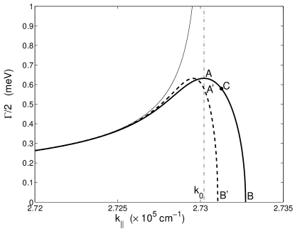
Figure 1: The radiative half-width $\Gamma/2=\Gamma_{\rm T}/2$ of $Y$-polarized QW excitons against the in-plane wavevector $k_{\parallel}$, evaluated with the standard perturbative approach given by Eq. (6) (thin solid line), the self-consistent perturbation approach given by Eq. (11) (dashed line), and by the exact diagonalization of the Hamiltonian (1), i.e., by Eq. (5) (solid line). The dashed-dotted vertical line indicates $k_{0}=k(\omega_{0})=(\sqrt{\varepsilon_{\rm{b}}}\omega_{0})/(\hbar c)$. In numerical calculations we use $R_{\rm QW}=0.025\,\mbox{eV}^{2}\rm\AA$ and $\omega_{0}=1.5$ eV, so that $\Gamma_{0}=45.5\,\mu$eV and the intrinsic radiative lifetime of QW excitons is given by $\tau_{\rm R}=\hbar/\Gamma_{0}=14.5$ ps. The critical points $A$ ($A^{\prime}$), $B$ ($B^{\prime}$), and $C$ are specified in the text.

In order to understand the removal of $(k_{0}^{2}-k_{\|}^{2})^{-1/2}$ divergence which appears in the perturbative approach given by Eq. (6), we examine the joint density of states (JDS), $\rho({\bf k}_{\|},\omega)$, for the resonant optical decay of QW excitons in the bulk photon modes:

$$\rho\big{(}\textbf{k}_{\parallel},\omega=\omega_{\textbf{{k}}_{\parallel}}^{\rm x}\big{)}\propto{1\over\pi}\int_{-\infty}^{+\infty}dk_{z}\,\frac{\gamma}{\gamma^{2}+\big{(}\omega_{\textbf{{k}}_{\parallel}}^{\rm x}-\omega^{\gamma}_{\textbf{{k}}}\big{)}^{2}}\,,$$ (10)

where $2\gamma=\gamma_{\rm x}+\Gamma$ is the total scattering rate of QW excitons. When $\partial\omega^{\gamma}_{\textbf{{k}}}(k_{\parallel},k_{z})/\partial k_{z}\neq 0$ at $k_{z}$ given by the energy conservation law $\omega_{\textbf{{k}}_{\parallel}}^{\rm x}(k_{\parallel})=\omega^{\gamma}_{\textbf{{k}}}(k_{\parallel},k_{z})$, the integrand function on the right-hand side (r.h.s) of Eq. (10) preserves its Lorentzian shape even in terms of $k_{z}$. In this case $\rho(\mathbf{k}_{\parallel})$ does not depend on $\gamma$, and the perturbative approach with Eq. (6) is valid. The situation is different when $k_{\parallel}\rightarrow k_{0}$: the solution of the energy conservation equation $\omega_{\textbf{{k}}_{\parallel}}^{\rm x}(k_{\parallel})=\omega^{\gamma}_{\textbf{{k}}}(k_{\parallel}=k_{0},k_{z})$ is $k_{z}=0$, and $\partial\omega^{\gamma}_{\textbf{{k}}}(k_{\parallel}=k_{0},k_{z})/\partial k_{z}=0$, indicating a one-dimensional (1D) van Hove singularity in the joint density of states. Thus $\rho(\mathbf{k}_{\parallel},\omega=\omega_{\textbf{{k}}_{\parallel}}^{\rm x})$ becomes $\gamma$-dependent in the vicinity of $k_{\parallel}=k_{0}$.

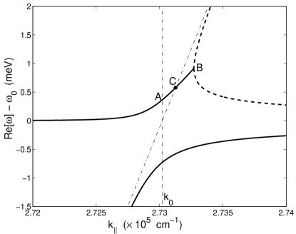
Figure 2: The polariton dispersion Re$[\omega]-\omega_{0}$, i.e., the Lamb shift $\Delta=\Delta_{\rm T}$ of optically-dressed $Y$-polarized QW excitons against the in-plane wavevector $k_{\parallel}$. The numerical calculations are done with the dispersion Eq. (5), the upper (lower) solid line refers to the radiative (confined) polariton states. The dash-dotted line shows the dispersion of bulk photons, $(\hbar ck_{\parallel}/\sqrt{\varepsilon_{\rm{b}}})-\omega_{0}$. The dashed two-branch dispersion curve beyond the terminal, bifurcation point $B$ is relevant to the radiative states and has no physical meaning for $\gamma_{\rm x}=0$ (see Sec. V). The segment $CB$ refers to the radiative states located outside the photon cone.

By applying standard perturbation theory with the JDS determined by Eq. (10), one receives for the optical decay of QW excitons:

$$\Gamma_{\rm T}(k_{\parallel})=\frac{(\sqrt{2}k_{0}^{2}k_{\parallel}\tilde{\gamma})\Gamma_{0}}{\big{[}(k_{0}^{2}-k_{\parallel}^{2})^{2}+4\tilde{\gamma}^{2}k_{0}^{2}k_{\parallel}^{2}\big{]}^{1/2}\,\big{[}[(k_{0}^{2}-k_{\parallel}^{2})^{2}+4\tilde{\gamma}^{2}k_{0}^{2}k_{\parallel}^{2}]^{1/2}-(k_{0}^{2}-k_{\parallel}^{2})\big{]}^{1/2}}\,,$$ (11)

where $\tilde{\gamma}=\gamma/\omega_{0}$, $\delta=k_{\parallel}/k_{0}=(\hbar ck_{\parallel})/(\sqrt{\varepsilon_{\rm{b}}}\omega_{0})$, and $\tilde{\delta}=\sqrt{1-\delta^{2}}$ ($\tilde{\delta}=\sqrt{\delta^{2}-1}$) for $k_{\parallel}\leq k_{0}$ ($k_{\parallel}>k_{0}$). The regular perturbative solution (see the dashed line in Fig. 1) refers to $k_{\parallel}\lesssim k_{0}-\tilde{\gamma}k_{0}$ with the dimensionless parameter $\tilde{\gamma}=\gamma/\omega_{0}\sim 10^{-3}$. In this case, the JDS is given by $\rho=[(\varepsilon_{\rm{b}}\omega_{0})/(\pi c^{2}\hbar^{2})](k_{0}^{2}-k_{\parallel}^{2})^{-1/2}$ and Eq. (11) reduces to Eq. (6). In contrast, for the narrow wavevector band $|k_{\parallel}-k_{0}|\lesssim\tilde{\gamma}k_{0}$ the 1D van Hove singularity strongly affects the radiative corrections. In particular, for $k_{\parallel}=k_{0}$ Eqs. (10) and (11) yield

$$\rho(k_{\parallel}=k_{0})=\frac{\sqrt{\varepsilon_{\rm{b}}}}{2\pi\hbar c}\,\frac{1}{\sqrt{\tilde{\gamma}}}\ \ \ \ \mbox{and}\ \ \ \ \Gamma_{\rm{T}}(k_{\parallel}=k_{0})=\frac{\Gamma_{0}}{2\sqrt{\widetilde{\gamma}}}\,.$$ (12)

Equations (12) clearly show that the scattering processes relax the 1D van Hove singularity at $k_{\parallel}=k_{0}$ and give rise to a finite value of $\Gamma_{\rm{T}}(k_{\parallel}=k_{0})\propto 1/\gamma^{1/2}$.

For the completely coherent interaction of QW excitons with bulk photons, when $\gamma_{\rm x}=0$, Eq. (11) can also be interpreted in terms of “self-consistent” perturbation theory. In this case, $\tilde{\gamma}=\Gamma_{\rm T}/(2\omega_{0})$ and for the band $|k_{\parallel}-k_{0}|\lesssim\tilde{\gamma}k_{0}$ the radiative width $\Gamma_{\rm T}=\Gamma_{\rm T}(k_{\parallel})$ should be found as a solution of Eq. (11) with the right-hand side (r.h.s.) explicitly dependent on $\Gamma_{\rm T}$. This solution is well approximated by using a real root of the cubic equation, $x^{2}(x+\varepsilon)=\Gamma_{0}^{2}/(16\omega_{0}^{2})$, with $x=\sqrt{\varepsilon^{2}+\Gamma_{\rm T}^{2}/(4\omega_{0}^{2})}$ and $\varepsilon=(k_{\parallel}-k_{0})/k_{0}$ ($|\varepsilon|\lesssim\tilde{\gamma}$). The radiative width $\Gamma_{\rm T}=\Gamma_{\rm T}(k_{\parallel})$ numerically evaluated with the self-consistent perturbation theory is shown in Fig. 1 by the dashed line. The self-consistent perturbation theory reproduces qualitatively the exact solution of Eq. (5) for the radiative states (solid line in Fig. 1). In particular, for $k_{\parallel}=k_{0}$ the self-consistent perturbative Eqs. (12) with $\tilde{\gamma}=\Gamma_{\rm T}/(2\omega_{0})$ yield $\Gamma_{\rm T}(k_{\parallel}=k_{0})=(1/\sqrt[3]{2})\,\big{(}\Gamma_{0}^{2}\omega_{0}\big{)}^{1/3}$, a value by only 8% smaller than the exact one, $\Gamma_{\rm T}^{\rm(A)}$, given by Eqs. (7) (see points $A$ and $A^{\prime}$ in Fig. 1).

It is the scattering-induced relaxation of energy conservation in the resonant conversion “QW exciton $\leftrightarrow$ bulk photon”, $\omega_{\textbf{{k}}_{\parallel}}^{\rm x}~{}(\simeq\omega_{0})=\hbar(c/\sqrt{\varepsilon_{\rm{b}}})\sqrt{k_{\parallel}^{2}+k_{z}^{2}}$, that is responsible for the appearance of the radiative states beyond the photon cone, i.e., beyond the point $C$ in Figs. 1 and 2. Furthermore, even for $\gamma_{\rm x}=0$ the coherent optical decay itself relaxes energy conservation, putting the quasi-eigenenergies of the radiative states in the complex plane (of course, the energy is strictly conserved in the incoming and outgoing channels of the scattering process “incoming bulk photon $\rightarrow$ QW exciton $\rightarrow$ outgoing bulk photon”). A straightforward analysis of Eq. (10) shows the existence of the JDS relevant to the resonant coupling of QW excitons and bulk photons even beyond the photon cone, if $\gamma$ is nonzero, and qualitatively justifies the asymptotic $\Gamma_{\rm T}\propto\sqrt{k_{\|}^{\rm(B)}-k_{\parallel}}$ [see Eq. (9)] which is valid for $k_{0}<k_{\parallel}\leq k_{\|}^{\rm(B)}$.

For the strong coupling limit of QW excitons and bulk photons ($\gamma_{\rm x}=0$), the width $\Gamma_{\rm T}$ and Lamb shift $\Delta_{\rm T}$ of the radiative states at $k_{\parallel}\simeq k_{0}$ are uniquely scaled by the control parameter $\big{(}\Gamma_{0}^{2}\omega_{0}\big{)}^{1/3}$ [see Eqs. (7)-(8)]. Furthermore, the maximum radiative width $\Gamma_{\rm T}^{\rm max}=\Gamma_{\rm T}^{\rm(A)}$ cannot screen completely the maximum radiative blue shift $\Delta_{\rm T}^{\rm max}=\Delta_{\rm T}^{\rm(B)}$, because the shift – half-width ratio $2\Delta_{\rm T}^{\rm max}/\Gamma_{\rm T}^{\rm max}=(2\sqrt[3]{2})/\sqrt{3}\simeq 1.5$, according to Eqs. (7)-(8). The radiative corrections can be seen experimentally for high-quality GaAs quantum wells even with a relatively small oscillator strength of QW excitons. For example, for the parameters used in our evaluations we estimate $\big{(}\Gamma_{0}^{2}\omega_{0}\big{)}^{1/3}\simeq 1.46$ meV, $\Gamma_{\rm T}^{\rm max}/2\simeq 0.63$ meV, and $\Delta_{\rm T}^{\rm max}\simeq 0.92$ meV.

IV Strong-weak coupling transition for quantum well polaritons

In this Section, in order to study how the QW polariton effect relaxes with increasing damping, we analyze the dispersion Eq. (5) with a nonzero excitonic damping $\gamma_{\rm x}$. Following the terminology developed by Tait Tait for bulk polaritons, two cases are distinguished: the quasi-particle solution $\omega=\omega(k_{\|})$ (wavevector $k_{\|}$ is real) and the forced-harmonic solution $k_{\|}=k_{\|}(\omega)$ (frequency $\omega$ is real).

IV.1 Quasi-particle solutions for quantum well polaritons

For QW polaritons, the true solutions $\omega=\omega(k_{\parallel})$ of Eq. (5) have to satisfy the following conditions: $\mbox{Re}[\kappa]\equiv\mbox{Re}\big{[}\sqrt{k_{\parallel}^{2}-k^{2}(\omega)}\big{]}\geq 0$ and $\mbox{Im}[\omega]\leq 0$. The first criterion ensures that the light field associated with QW polaritons has an evanescent envelope in the $z$-direction, $E(z)=E(0)\exp(-\kappa|z|)$, while the second one stems from the casuality principle. For small $\gamma_{\rm x}$, there is only one dispersion branch which is relevant to QW polaritons, $\omega=\omega_{1}(k_{\parallel})$ (see the r.h.s. solid line $n$ in Fig. 3), as detailed, e.g., in Refs. [Orrit, ; Nakayama, ; Andreania, ; Andreanib, ] for $\gamma_{\rm x}=0$. However, for $\gamma_{\rm x}=\gamma_{\rm c}^{(1)}$ a new, second dispersion branch of QW polaritons, $\omega=\omega_{2}(k_{\|})$, emerges and develops with increasing $\gamma_{\rm x}\geq\gamma_{\rm c}^{(1)}$ (see the left-hand side lines $a$ in Fig. 3). The critical rate $\gamma_{\rm c}^{(1)}$ of incoherent scattering is given by

$$\gamma_{\rm x}=\gamma_{\rm c}^{(1)}=R_{\rm QW}\,\frac{\sqrt{\varepsilon_{\rm b}}}{\hbar c}=\Gamma_{0}\,,$$ (13)

i.e., is exactly equal to the intrinsic radiative width of QW excitons with $k_{\parallel}=0$. The second dispersion branch has two symmetric terminal points $A_{\rm f}^{\prime}$ and $A_{\rm f}$ at $k_{\parallel}=\pm k_{\parallel}^{\rm f}$ (the point $A_{\rm f}^{\prime}$ is not shown in Fig. 3), where $k_{\parallel}^{\rm f}$ is given by

$$k_{\parallel}^{\rm f}=k_{\parallel}^{\rm f}(\gamma_{\rm x}\geq\gamma_{\rm c}^{(1)}\!=\!\Gamma_{0})=\omega_{0}\frac{\sqrt{\varepsilon_{\rm b}}}{\hbar c}\sqrt{1-{\varepsilon_{\rm b}R_{\rm QW}^{2}\over\gamma_{\rm x}^{2}\hbar^{2}c^{2}}}=k_{0}\sqrt{1-\left({\Gamma_{0}\over\gamma_{\rm x}}\right)^{2}}\,,$$ (14)

The terminal points $A_{\rm f}^{\prime}$ and $A_{\rm f}$ are characterized by Re$[\omega_{2}(k_{\|}\!=\!\pm k_{\|}^{\rm f})]=\sqrt{\omega_{\textbf{{k}}_{\parallel}}^{\rm x}-\gamma_{\rm x}^{2}}\simeq\omega_{0}$, Im$[\omega_{2}(k_{\|}\!=\!\pm k_{\|}^{\rm f})]=0$ and $\textrm{Re}[\kappa(k_{\parallel}\!=\!\pm k_{\parallel}^{\rm f})]=0$. In addition, the middle point $A_{\rm i}$ of the segment $A_{\rm f}^{\prime}A_{\rm f}$ is specified by $k_{\parallel}=k_{\parallel}^{\rm i}=0$ and Re$[\omega_{2}(k_{\parallel}\!=\!0)]=\sqrt{\omega_{0}^{2}-\Gamma_{0}^{2}}\simeq\omega_{0}$ (see Fig. 3).

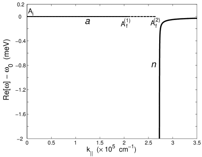
Figure 3: The quasi-particle dispersion branches of QW polaritons, $\mbox{Re}[\omega]=\mbox{Re}[\omega(k_{\|})]$, evaluated with Eq. (5). The solid curve $n$ shows the normal QW polariton dispersion branch calculated for $\gamma_{\rm x}=0$. The solid (dashed) curve $a$ refers to the anomalous, $\gamma_{\rm x}$-induced QW polariton dispersion branch calculated for $\gamma_{\rm x}=70\,\mu$eV ($\gamma_{\rm x}=200\,\mu$eV). The critical damping $\gamma_{\rm c}^{(1)}=\Gamma_{0}=45.5\,\mu$eV.

At marginal points $A_{\rm f}^{\prime}$ and $A_{\rm f}$ (see Fig. 3), which are characterized by Im$[\omega_{2}]=0$, the anomalous, damping-induced dispersion branch $\omega=\omega_{2}(k_{\|})$ appears from and leaves for the unphysical part of 3D space $\{k_{\|},\mbox{Im}[\omega],\mbox{Re}[\omega]\}$. The dispersion Eq. (5) can easily be transformed to a cubic equation, generally with complex coefficients, for $\omega^{2}=\omega^{2}(k_{\parallel})$. For $\gamma_{\rm x}=0$, when the coefficients are real, one of the roots of this equation is characterized by Im$[\omega^{2}]=0$ and corresponds to QW polaritons, while second and third roots are complex conjugated. Among the latter two solutions, one of the roots satisfies the selection criteria for radiative polaritons, as discussed in Sec. V, giving rise to the radiative state, while another one is unphysical. For $\gamma_{\rm x}\geq\gamma_{\rm c}^{(1)}=\Gamma_{0}$, the unphysical branch evolves in $\{k_{\|},\mbox{Im}[\omega],\mbox{Re}[\omega]\}$ space in such a way that it has a segment where the criteria for QW polaritons are met. Similarly to the radiative states which can exist beyond the photon cone, the appearance of the second dispersion branch of QW polaritons within the photon cone is due to relaxation of the energy conservation $\delta$-function by the damping rate $\gamma_{\rm x}$. Because $\mbox{Re}[\omega_{2}]\simeq\omega_{0}$, the anomalous dispersion branch can be interpreted in terms of a new, damping-induced optical decay channel of the exciton states that opens up and develops with increasing $\gamma_{\rm x}\geq\gamma_{\rm c}^{(1)}$. In this case, a QW exciton with momentum $k_{\|}<k_{0}$, i.e., within the photon cone, can directly emit an interface photon of the evanescent light field. The damping-induced dispersion branches are known in plasma physics [Shivarova, ] and in physics of the surface electromagnetic waves [Halevi1, ; Halevi2, ].

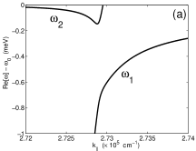
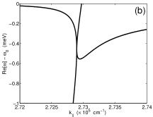
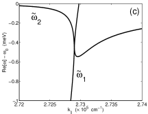
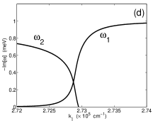
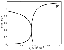
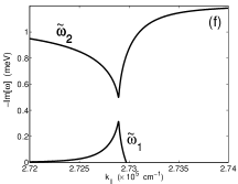
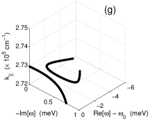
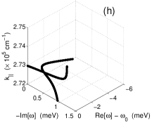
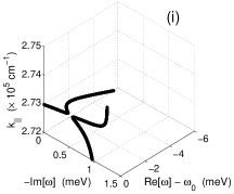
Figure 4: The damping-induced transition between the strong and weak coupling limits for quasi-particle QW polaritons [$\omega=\omega(k_{\|})$ is a solution of the dispersion Eq. (5) parametrically dependent upon real $k_{\|}$]. For $R_{\rm QW}=0.025\,\mbox{eV}^{2}\rm\AA$, the transition damping rate is given by $\gamma_{\rm x}^{\rm tr}=\gamma_{\rm c}^{(2)}\simeq 2.39$ meV, according to Eqs. (15). (a), (d), (g): The strong coupling regime, $\gamma_{\rm x}=2.20\,\mbox{meV}<\gamma_{\rm c}^{(2)}$. (b), (e), (h): The transition point, $\gamma_{\rm x}=\gamma_{\rm x}^{\rm tr}=\gamma_{\rm c}^{(2)}$. (c), (f), (i): The weak coupling regime, $\gamma_{\rm x}=2.44\,\mbox{meV}>\gamma_{\rm c}^{(2)}$.

With increasing $\gamma_{\rm x}\geq\gamma_{\rm c}^{(1)}$, the two dispersion curves, $\omega_{1}=\omega_{1}(k_{\|})$ and $\omega_{2}=\omega_{2}(k_{\|})$, move in 3D space $\{k_{\|},\mbox{Im}[\omega],\mbox{Re}[\omega]\}$ towards each other (see Fig. 4). The intersection of the dispersion curves, which occurs for $\gamma_{\rm x}=\gamma_{\rm x}^{\rm tr}=\gamma_{\rm c}^{(2)}$, is interpreted as a transition between the strong ($\gamma_{\rm x}\leq\gamma_{\rm c}^{\rm tr}$) and weak ($\gamma_{\rm x}\geq\gamma_{\rm c}^{\rm tr}$) coupling limits of QW exciton – photon interaction. According to the dispersion Eq. (5), there is only one intersection point, which is given by the conditions $\mbox{Re}[\omega_{1}(k_{\|},\gamma_{\rm x}^{\rm tr})]=\mbox{Re}[\omega_{2}(k_{\|},\gamma_{\rm x}^{\rm tr})]$ and $\mbox{Im}[\omega_{1}(k_{\|},\gamma_{\rm x}^{\rm tr})]=\mbox{Im}[\omega_{2}(k_{\|},\gamma_{\rm x}^{\rm tr})]$ [see Figs. 4(b), 4(e) and 4(h)]. These conditions define the transition parameters:

$$\gamma_{\rm x}^{\rm tr} = \gamma_{\rm c}^{(2)}=\frac{3\sqrt{3}}{2}\,\left(\frac{\omega_{0}R_{\rm QW}^{2}\varepsilon_{\rm b}}{4c^{2}\hbar^{2}}\right)^{1/3}\!\!={3\sqrt{3}\over 2\sqrt[3]{4}}\,\big{(}\Gamma_{0}^{2}\omega_{0}\big{)}^{1/3}\simeq 1.64\,\big{(}\Gamma_{0}^{2}\omega_{0}\big{)}^{1/3}\,,$$

$$k_{\|}^{\rm tr} = k_{0}\left[1-{1\over\sqrt{3}}\,{\gamma_{\rm c}^{(2)}\over\omega_{0}}\right]=k_{0}-{3\over 2\sqrt[3]{4}}\,{\sqrt{\varepsilon_{\rm{b}}}\over\hbar c}\,\big{(}\Gamma_{0}^{2}\omega_{0}\big{)}^{1/3}\,.$$ (15)

The transition point is characterized by the complex polariton frequency $\omega(k_{\|}^{\rm tr})=\omega_{1}(k_{\|}^{\rm tr})=\omega_{2}(k_{\|}^{\rm tr})$ given by

$$\Delta_{\rm T}^{\rm tr} = \mbox{Re}[\omega(k_{\|}^{\rm tr})]-\omega_{0}=-{1\over\sqrt[3]{4}}\,\big{(}\Gamma_{0}^{2}\omega_{0}\big{)}^{1/3}\,,$$

$$\Gamma_{\rm T}^{\rm tr} = -2\,\mbox{Im}[\omega(k_{\|}^{\rm tr})]={2\over 3}\,\gamma_{\rm c}^{(2)}={\sqrt{3}\over\sqrt[3]{4}}\,\big{(}\Gamma_{0}^{2}\omega_{0}\big{)}^{1/3}\,.$$ (16)

For the parameters used in our numerical evaluations, $\gamma_{\rm x}^{\rm tr}=\gamma_{\rm c}^{(2)}\simeq 2.39$ meV, $\Delta_{\rm T}^{\rm tr}\simeq-0.92$ meV, and $\Gamma_{\rm T}^{\rm tr}\simeq 1.59$ meV.

At the intersection point between two dispersion curves, when $\gamma_{\rm x}=\gamma_{\rm x}^{\rm tr}$, the interconnection between the dispersion branches changes from “anti-crossing” (strong coupling regime) to “crossing” (weak coupling regime). As a result, topologically new dispersion branches, $\tilde{\omega}_{1}(k_{\|})$ and $\tilde{\omega}_{2}(k_{\|})$, arise for $\gamma_{\rm x}>\gamma_{\rm x}^{\rm tr}$ (see Fig. 4). For example, for $\gamma_{\rm x}=0$ the only QW polariton dispersion branch $\omega_{1}=\omega_{1}(k_{\|})$ can be interpreted in terms of photon-like [$k_{\|}\lesssim k_{0}=k_{0}$] and exciton-like ($k_{\|}\gtrsim k_{0}$) parts [“anti-crossing” of the exciton and photon dispersions, see Fig. 4 (a)]. In contrast, for $\gamma_{\rm x}\gtrsim\gamma_{\rm x}^{\rm tr}$, i.e., after the transition, the new dispersion branch $\tilde{\omega}_{1}(k_{\parallel})$, which starts at $k_{\|}=0$ with $\tilde{\omega}_{1}=0$ and terminates at $k_{\|}=k_{\|}^{\rm f}(\gamma_{\rm x})\simeq k_{0}$ [for $\gamma_{\rm x}\gg\gamma_{\rm c}^{(2)}=\gamma_{\rm x}^{\rm tr}$, Eq. (14) yields $k_{\|}^{\rm f}\rightarrow k_{0}$] with $\tilde{\omega}_{1}\simeq\omega_{0}$, can be visualized as a purely photon-like branch [“crossing” of the exciton and photon dispersions, see Fig. 4 (c)]. In a similar way, the entire $\tilde{\omega}_{2}$-branch can be interpreted in terms of the exciton dispersion.

IV.2 Forced-harmonic solutions for quantum well polaritons

For quasi-2D QW polaritons, the forced-harmonic solutions $k_{\parallel}=k_{\parallel}(\omega)$ of Eq. (5) should satisfy the following conditions: Re$[\kappa]\geq 0$ and Im$[k_{\parallel}]\geq 0$. Comparing with the quasi-particle solutions, an additional dimensionless parameter $\nu_{\rm x}=(\omega_{0}\varepsilon_{\rm{b}})/(M_{\rm x}c^{2})$ is relevant to this class of solutions. The parameter $\nu_{\rm x}$ explicitly depends on the translational mass of QW excitons, so that $\nu_{\rm x}\rightarrow 0$ for $M_{\rm x}\rightarrow\infty$. For the control parameters relevant to GaAs QWs, one estimates $\nu_{\rm x}\simeq(1.2-1.3)\times 10^{-4}$.

Similarly to the quasi-particle solutions, a new dispersion branch $k_{\parallel}^{(2)}=k_{\parallel}^{(2)}(\omega)$ emerges with increasing $\gamma_{\rm x}\geq\tilde{\gamma}_{\rm c}^{(1)}$. In this case, however, $\tilde{\gamma}_{\rm c}^{(1)}=0$, and the anomalous dispersion branch starts to develop from $\{k_{\parallel}^{\rm i}\!=\!0,\omega^{\rm i}\!=\!0\}$ point. For a given incoherent scattering rate $\gamma_{\rm x}>0$, the terminal point $A_{\rm f}$, where the $\gamma_{\rm x}$-induced branch leaves for the unphysical part of 3D space $\{\omega,\mbox{Im}[k_{\|}],\mbox{Re}[k_{\|}]\}$ (see Figs. 5 and 6), is characterized by the frequency

$$\omega=\omega^{\rm f}(\gamma_{\rm x})=\frac{\omega_{0}}{\big{[}1-\nu_{\rm x}+\nu_{\rm x}(\Gamma_{0}/\gamma_{\rm x})^{2}\big{]}^{1/2}}\,.$$ (17)

Equation (17), which is valid for $\nu_{\rm x}\ll 1$, indeed shows that $\tilde{\gamma}_{\rm c}^{(1)}=0$: $\omega^{\rm f}\rightarrow 0$ for $\gamma_{\rm x}\rightarrow 0$. For $\gamma_{\rm x}\gtrsim\Gamma_{0}$, when frequency $\omega^{\rm f}$ approaches $\omega_{0}$ (see Fig. 5), Eq. (17) reduces to

$$\omega=\omega^{\rm f}(\gamma_{\rm x}\!\gtrsim\,\Gamma_{0})=\omega_{0}\Bigg{[}1+{\nu_{\rm x}\over 2}\bigg{[}1-\bigg{(}{\Gamma_{0}\over\gamma_{\rm x}}\bigg{)}^{2}\,\bigg{]}\Bigg{]}\,.$$ (18)

For the terminal point $A_{\rm f}$ of the anomalous dispersion branch, which is characterized by $k_{\parallel}^{\rm f}=\{\mbox{Re}[k_{\parallel}(\omega^{\rm f})],\mbox{Im}[k_{\parallel}(\omega^{\rm f})]\}$, one has $\mbox{Im}[k_{\parallel}(\omega^{\rm f})]=0$ and $\mbox{Re}[\kappa]=0$, and Eq. (18) yields

$$\mbox{Re}[k_{\parallel}^{(2)}(\omega^{\rm f})]=k_{0}\Bigg{[}1+{\nu_{\rm x}\over 2}\bigg{[}1-\bigg{(}{\Gamma_{0}\over\gamma_{\rm x}}\bigg{)}^{2}\,\bigg{]}\Bigg{]}\,.$$ (19)

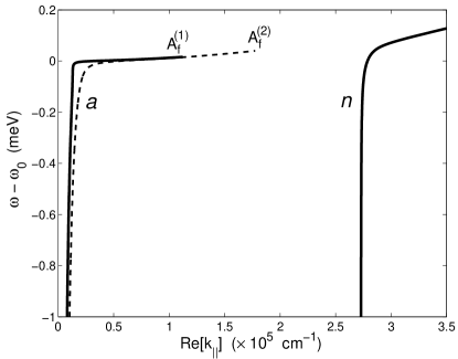
Figure 5: The forced-harmonic dispersion branches of QW polaritons, $\mbox{Re}[k_{\parallel}]=\mbox{Re}[k_{\parallel}(\omega)]$. The solid line $n$ refers to the normal QW polariton dispersion branch calculated with Eq. (5) for $\gamma_{\rm x}=0$. The solid (dashed) line $a$ is the anomalous, damping-induced dispersion branch of QW polaritons evaluated for $\gamma_{\rm x}=50\,\mu$eV ($\gamma_{\rm x}=60\,\mu$eV). The in-plane translational mass of QW excitons is given by $M_{\rm x}=0.3\,m_{0}$, where $m_{0}$ is the free electron mass.

Similar to the case of the quasi-particle solutions, the transition between the strong and weak coupling regimes of the QW exciton – photon interaction is attributed to the intersection of the two dispersion curves, $k_{\|}^{(1)}(\omega)$ and $k_{\|}^{(2)}(\omega)$, in 3D space $\{\omega,\mbox{Im}(k_{\|}),\mbox{Re}(k_{\|})\}$ (see Fig. 6). Thus the topologically new dispersion branches ${\tilde{k}_{\parallel}}^{(1)}(\omega)$ and ${\tilde{k}_{\parallel}}^{(2)}(\omega)$ arise from the old ones, $k_{\|}^{(1)}(\omega)$ and $k_{\|}^{(2)}(\omega)$, with $\gamma_{\rm x}$ increasing above $\tilde{\gamma}_{\rm x}^{\rm tr}=\tilde{\gamma}_{\rm c}^{(2)}$. The transition point is given by

$$\tilde{\gamma}_{\rm x}^{\rm tr} = \tilde{\gamma}_{\rm c}^{(2)}\ =\ \frac{3\sqrt{3}}{2}\,\left(\frac{\omega_{0}^{2}R_{\rm QW}^{2}\varepsilon_{\rm b}^{2}}{c^{4}\hbar^{2}M_{\rm x}}\right)^{1/3}=\,\sqrt[3]{4}\,\nu_{\rm x}^{1/3}\gamma_{\rm c}^{(2)}\,,$$ (20)

$$\omega^{\rm tr} = \omega_{0}\left[1+{\omega_{0}\varepsilon_{\rm b}\over 2c^{2}M_{\rm x}}-{1\over\sqrt{3}\sqrt[3]{32}}\,{\tilde{\gamma}_{\rm c}^{(2)}\over\omega_{0}}\right]\,.$$ (21)

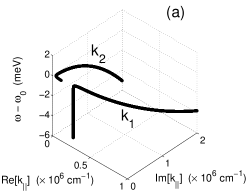
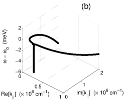
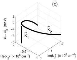
Figure 6: The $\gamma_{\rm x}$-induced transition between the strong and weak coupling limits for forced-harmonic QW polaritons. For $R_{\rm QW}=0.025\,\mbox{eV}^{2}\AA$ and $M_{\rm x}=0.3\,m_{0}$, the critical value of the damping rate is given by $\tilde{\gamma}_{\rm x}^{\rm tr}=\tilde{\gamma}_{\rm c}^{(2)}=119.8\,\mu$eV, according to Eq. (20). (a) The strong coupling regime, $\gamma_{\rm x}<\tilde{\gamma}_{\rm c}^{(2)}$, (b) the transition point, $\gamma_{\rm x}=\tilde{\gamma}_{\rm x}^{\rm tr}=\tilde{\gamma}_{\rm c}^{(2)}$, and (c) the weak coupling regime, $\gamma_{\rm x}>\tilde{\gamma}_{\rm c}^{(2)}$.

In contrast with the quasi-particle solution, for the forced-harmonic solution the transition point is very sensitive to the in-plane translational mass $M_{\rm x}$ of QW excitons: $\tilde{\gamma}_{\rm x}^{\rm tr}\propto M_{\rm x}^{-1/3}$, according to Eq. (20). In particular, when $M_{\rm x}\rightarrow\infty$ and therefore the spatial dispersion due to excitons is removed, one has $\tilde{\gamma}_{\rm x}^{\rm tr}=0$. In this case, the integrated absorption associated with the exciton-like branch, ${\tilde{k}_{\parallel}^{(2)}}={\tilde{k}_{\parallel}^{(2)}}(\omega)$, is constant independent of the damping rate $\gamma_{\rm x}$: $\int\mbox{Im}[{\tilde{k}_{\parallel}^{(2)}}(\omega)]d\omega=const\propto R_{\rm QW}$. This sum rule for the absorption coefficient is known for bulk [Loudon, ] and QW [Andreanie, ] excitons. Note that the large difference between the critical damping rates $\gamma_{\rm x}^{\rm tr}=\gamma_{\rm c}^{(2)}$ and $\tilde{\gamma}_{\rm x}^{\rm tr}=\tilde{\gamma}_{\rm c}^{(2)}$ ($\gamma_{\rm x}^{\rm tr}\gg\tilde{\gamma}_{\rm x}^{\rm tr}$, e.g., for our numerical evaluations one has $\gamma_{\rm x}^{\rm tr}\simeq 2.4$ meV against $\tilde{\gamma}_{\rm x}^{\rm tr}\simeq 0.12$ meV), which refer to the quasi-particle (photoluminescence experiment) and forced-harmonic (optical reflectivity/transmissivity experiment) solutions, respectively, is well-known for bulk polaritons Tait .

IV.3 Optical brightness of damping-induced quantum well polaritons

One can naturally question to what extent the $\gamma_{\rm x}$-induced QW polariton dispersion branch is observable, i.e., “physical”. Some aspects of this question are discussed in Sec. VI. Here, we analyze the photon component $\varphi^{\gamma}_{\rm 2D}$ along the normal and anomalous QW polariton dispersion branches. The photon component is a measure of the brightness of polaritons.

In the initial Hamiltonian, Eqs. (1)-(2), quasi-2D excitons couple with bulk photons. However, the confined QW polariton modes deal with the quasi-2D light field: In this case the QW excitons are dressed by the evanescent electromagnetic field which in turn is trapped and guided by the QW exciton states. The area-density of the electromagnetic energy $W^{\rm 2D}_{\rm phot}$, associated with the evanescent light field, is given by

$$W_{\rm phot}^{\rm 2D}=\int_{-\infty}^{+\infty}\!\big{(}W_{\rm E}^{\rm 3D}+W_{\rm H}^{\rm 3D}\big{)}\,dz=\frac{1}{4\pi}\frac{|E(0)|^{2}}{\rm{Re}[\kappa]}\,,$$ (22)

so that the dimensionless amplitude of the quasi-2D light field is defined as

$$e^{\rm 2D}_{{\textbf{{k}}}_{\|}}=\left(\frac{2}{L\rm{Re}[\kappa]}\right)^{1/2}\sum_{k_{z}}\bigg{(}{\omega_{0}\over\omega_{{\textbf{{k}}}_{\|}}^{\gamma}}\bigg{)}^{1/2}\!\big{(}\alpha_{{\textbf{{k}}}_{\|},k_{z}}+\alpha_{\textbf{{-k}}_{\|},-k_{z}}^{{\dagger}})\,.$$ (23)

The amplitude $e^{\rm 2D}_{{\textbf{{k}}}_{\|}}$ can also be interpreted as a combination of the creation and annihilation operators of the quasi-2D photons. In a similar way, the dimensionless amplitude of the quasi-2D excitonic polarization is given by the operator $x^{\rm 2D}_{{\textbf{{k}}}_{\|}}=i(b_{{\textbf{{k}}}_{\|}}-b^{{\dagger}}_{-{\textbf{{k}}}_{\|}})$.

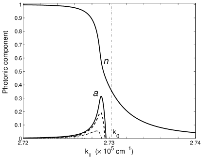
Figure 7: The photon component $\varphi^{\gamma}_{\rm 2D}=\varphi^{\gamma}_{\rm 2D}(k_{\|})$ of the normal and anomalous, damping-induced branches for $\gamma_{\rm x}=2.2$ meV (solid lines), and of the anomalous branch for $\gamma_{\rm x}=2.0$ meV (dashed line), $1.6$ meV (dashed-dotted line), and $1.0$ meV (dotted line). The position of the photon cone, $k_{\|}=k(\omega)$, is indicated by the vertical dash-dotted line.

Equations (1)-(2) yield the following relationship between $e^{\rm 2D}_{{\textbf{{k}}}_{\|}}$ and $x^{\rm 2D}_{{\textbf{{k}}}_{\|}}$:

$$\big{[}\omega^{2}-(\omega^{\rm x}_{{\textbf{{k}}}_{\|}})^{2}\big{]}x^{\rm 2D}_{{\textbf{{k}}}_{\|}}=\omega_{0}\big{(}R_{\rm QW}\mbox{Re}[\kappa]\big{)}^{1/2}e^{\rm 2D}_{{\textbf{{k}}}_{\|}}\,.$$ (24)

The photon and exciton component of quantum well polaritons are given by $\varphi^{\gamma}_{\rm 2D}(k_{\|})=|\tilde{e}^{\rm 2D}_{{\textbf{{k}}}_{\|}}|^{2}/(|\tilde{e}^{\rm 2D}_{{\textbf{{k}}}_{\|}}|^{2}+|\tilde{x}^{\rm 2D}_{{\textbf{{k}}}_{\|}}|^{2})$ and $\varphi^{\rm x}_{\rm 2D}(k_{\|})=1-\varphi^{\gamma}_{\rm 2D}=|\tilde{x}^{\rm 2D}_{{\textbf{{k}}}_{\|}}|^{2}/(|\tilde{e}^{\rm 2D}_{{\textbf{{k}}}_{\|}}|^{2}+|\tilde{x}^{\rm 2D}_{{\textbf{{k}}}_{\|}}|^{2})$, respectively. Here, $\tilde{e}^{\rm 2D}_{{\textbf{{k}}}_{\|}}$ and $\tilde{x}^{\rm 2D}_{{\textbf{{k}}}_{\|}}$ are the phase-synchronous components of the electric and polarization fields which contribute to the total stored energy of the quasi-2D system. Thus, by using Eq. (24), one derives:

$$\varphi^{\gamma}_{\rm 2D}(k_{\|})=\frac{\big{(}\mbox{Re}[\omega^{2}-(\omega^{\rm x}_{{\textbf{{k}}}_{\|}})^{2}]\big{)}^{2}}{\omega_{0}^{2}R_{\rm QW}\mbox{Re}[\kappa]+\big{(}\mbox{Re}[\omega^{2}-(\omega^{\rm x}_{{\textbf{{k}}}_{\|}})^{2}]\big{)}^{2}}\,.$$ (25)

For $\gamma_{\rm x}=0$, Eq. (25) reduces to the known expression for the photon component along the normal QW polariton dispersion branch [Orrit, ; Ivanov97, ; Ivanov98, ].

The photon component $\varphi^{\gamma}_{\rm 2D}$ along the anomalous ($a$) and normal ($n$) QW polariton dispersion branches, calculated with Eq. (25) for the quasi-particle solution of the dispersion Eq. (5), is plotted in Fig. 7 for various damping rates $\gamma_{\rm x}>\gamma_{\rm c}^{(1)}$. It is clearly seen that with increasing $\gamma_{\rm x}$ the damping-induced QW polariton states become bright, i.e., optically-active, only in close proximity of $k_{\|}=k_{0}$. At the crossover point $k_{\|}=k_{\|}^{\rm tr}$ of the dispersion branches, which occurs for $\gamma_{\rm x}=\gamma_{\rm x}^{\rm tr}=\gamma_{\rm c}^{(2)}$ [see Eqs. (15)], the brightness of the anomalous and normal QW polariton states becomes equal to each other. A similar behaviour of the photon component $\varphi^{\gamma}_{\rm 2D}$ of the QW polariton states takes place for the forced-harmonic solution $k_{\|}=k_{\|}(\omega)$ of Eq. (5).

V Strong-weak coupling transition for the radiative states

The damping-induced transition between the strong and weak coupling regimes of the QW-exciton – photon interaction can also be traced for the radiative states. The changes of the radiative width $\Gamma_{\rm T}=\Gamma_{\rm T}(k_{\parallel})$ and Lamb shift $\Delta_{\rm T}=\Delta_{\rm T}(k_{\parallel})$ with increasing $\gamma_{\rm x}$ are shown in Figs. 8(a)-(b). Here, the radiative corrections are defined as $\Gamma_{\rm T}=-2\mbox{Im}[\omega]-\gamma_{\rm x}$ and $\Delta_{\rm T}=\mbox{Re}[\omega]-\omega_{0}$, where $\omega$ is the solution of Eq. (5) that satisfies the following conditions: $\mbox{Re}[\kappa]\equiv\mbox{Re}\big{[}\sqrt{k_{\parallel}^{2}-k^{2}(\omega)}\big{]}\leq 0$ and $\mbox{Im}[\omega]\leq 0$. The solid lines in Figs. 8(a)-(b) (see also the solid line in Fig. 1 and the upper solid line in Fig. 2) refers to the completely coherent case, i.e., to the strong coupling limit with $\gamma_{\rm x}=0$, when the low-energy exciton state with $k_{\|}\leq k_{\|}^{\rm(B)}$ is dressed by outgoing bulk photons and interpreted as a radiative QW polariton. In this case, the point $B$ (see Figs. 1, 2, and 8) is the terminal point of the dispersion of the radiative states.

For an arbitrary small $\gamma_{\rm x}>0$ the dispersion of radiative polaritons persists beyond the point $B$, where the dispersion splits into two sub-branches, as a $\gamma_{\rm x}$-induced tail of the radiative states at $k_{\|}\geq k_{\|}^{\rm(B)}$. In this case, the upper dispersion sub-branch beyond the bifurcation point $B$ becomes unphysical, i.e., completely disappears, while the damping-induced radiative tail is associated with the lower dispersion sub-branch [see Figs. 8(a)-(b)]. The optical width $\Gamma_{\rm T}$ of the $\gamma_{\rm x}$-induced radiative states at $k_{\|}\geq k_{\|}^{\rm(B)}$ is approximated as

$$\Gamma_{\rm T}\big{(}k_{\parallel}>k_{\parallel}^{\rm(B)}\big{)}=\Gamma_{0}\,\bigg{(}\frac{\gamma_{\rm x}}{2\omega_{0}}\bigg{)}\bigg{(}\frac{k_{0}^{2}}{k_{\parallel}^{2}-k_{0}^{2}}\bigg{)}^{3/2}\,,$$ (26)

Approximation with Eq. (26) is valid provided that $(\hbar c/\sqrt{\varepsilon_{\rm{b}}})\sqrt{k_{\parallel}^{2}-k_{0}^{2}}\gg\gamma_{\rm x}$. Equation (26) clearly shows the damping-induced nature of the radiative tail: $\Gamma_{\rm T}\big{(}k_{\parallel}>k_{\parallel}^{\rm(B)}\big{)}$ is proportional to the incoherent damping rate $\gamma_{\rm x}$ and therefore vanishes when $\gamma_{\rm x}\rightarrow 0$. A similar $\gamma_{\rm x}$-induced tail of the radiative states has also been numerically found for quasi-one-dimensional plasmon-polaritons [Citrin2, ].

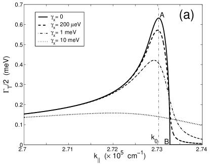
Figure 8: The dispersion of the $Y$-polarized radiative states (radiative polaritons) for $\gamma_{\rm x}=0$, 0.2 meV, 1 meV and 10 meV: (a) the radiative half-width $\Gamma/2=\Gamma_{\rm T}/2=-\mbox{Im}[\omega(k_{\parallel})]-\gamma_{\rm x}/2$ and (b) the radiative (Lamb) shift $\Delta=\Delta_{\rm T}=\mbox{Re}[\omega(k_{\parallel})]-\omega_{0}$. For the QW parameters see the caption of Fig. 1.

As shown in Figs. 8(a)-(b), in the vicinity of $k_{\parallel}=k_{0}$ the radiative corrections $\Gamma_{\rm T}$ and $\Delta_{\rm T}$ effectively decreases with increasing $\gamma_{\rm x}$. At the same time, there is no damping-induced anomalous branch for the radiative states of QW excitons. Therefore, in this case the transition between the strong and weak coupling regimes of exciton-photon interaction can only be approximately quantified in terms of the $\gamma_{\rm x}$-induced qualitative changes of the shape of the radiative corrections, $\Gamma_{\rm T}=\Gamma_{\rm T}(k_{\parallel})$ and $\Delta_{\rm T}=\Delta_{\rm T}(k_{\parallel})$, at $k_{\parallel}\simeq k_{0}$ [see, e.g., the solid against dotted lines in Figs. 8(a)-(b)]. The drastic, qualitative changes occur when the damping rate $\gamma_{\rm x}$ becomes comparable with the maximum radiative corrections, $\Gamma^{\rm A}_{\rm T}\propto\big{(}\Gamma_{0}^{2}\omega_{0}\big{)}^{1/3}$ given by Eq. (7) and $\Delta^{\rm B}_{\rm T}\propto\big{(}\Gamma_{0}^{2}\omega_{0}\big{)}^{1/3}$ given by Eq. (8). In order to attribute the transition to the critical damping $\gamma^{\rm tr}_{\rm x}=\gamma_{\rm x}^{(2)}\propto\big{(}\Gamma_{0}^{2}\omega_{0}\big{)}^{1/3}$ defined by Eq. (15) for confined QW polaritons, we choose the following criterion for the transition point:

$$\gamma_{\rm x}^{\rm tr}=\gamma_{\rm c}^{(2)}=\frac{3}{\sqrt[3]{4}}\,\Gamma_{\rm T}^{\rm A}\simeq 1.89\,\Gamma_{\rm T}^{\rm A}\,.$$ (27)

In this case, the transition occurs synchronously for both conjugated states, QW polaritons and radiative modes. As discussed in Sec. VI, the transition can be visualized in the angle-resolved photoluminescence signal from the radiative states of QW excitons.

VI DISCUSSION

The anomalous, damping-induced dispersion branch of QW polaritons can be visualized by using near-field or micrometric imaging spectroscopy techniques Hess ; Wu ; Pulizzi which allow to detect the evanescent light field associated with the QW polariton states. In Figs. 9 and 10 the evanescent field $E=E(z)=E(0)e^{-\mbox{\small Re}[\kappa]|z|}\cos\big{(}\mbox{Im}[\kappa]|z|\big{)}$ is plotted for the quasi-particle solution of the dispersion Eq. (5), for $\gamma_{\rm c}^{(1)}<\gamma_{\rm x}<\gamma_{\rm c}^{(2)}$ and $\gamma_{\rm x}\simeq\gamma_{\rm x}^{\rm tr}=\gamma_{\rm c}^{(2)}$, respectively. For $\gamma_{\rm c}^{(1)}<\gamma_{\rm x}\ll\gamma_{\rm c}^{(2)}$, the evanescent field associated with QW polaritons of the anomalous dispersion branch spatially oscillates with the period $2\pi/\mbox{Im}[\kappa]$ which is much less than the characteristic decay length of the envelope field, $1/\mbox{Re}[\kappa]$ (see the solid line in Fig. 9). A similar behaviour of the evanescent field is well-known in physics of surface acoustic waves Farnell . In spite of spatial oscillations of the evanescent field $E=E(z)$, there is, however, no energy flux in the normal, $z$-direction: The $\gamma_{\rm x}$-induced QW polariton states remain split off from the radiative modes. For the strong-weak coupling transition point, when $\gamma_{\rm x}=\gamma_{\rm x}^{\rm tr}$ and $k_{\parallel}=k_{\parallel}^{\rm tr}$ [see Eq. (15)], the evanescent fields associated with normal and anomalous QW polaritons become undistinguishable, as clearly illustrated in Fig. 10.

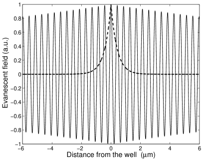
Figure 9: The evanescent light field profile $E=E(z)$ associated with normal (dashed line) and $\gamma_{\rm x}$-induced (solid line) QW polaritons. The damping rate corresponds to $\gamma_{\rm x}=1$ meV, while $\gamma^{(1)}_{\rm c}\simeq 0.046$ meV and $\gamma_{\rm x}^{\rm tr}=\gamma^{(2)}_{\rm c}\simeq 2.4$ meV.

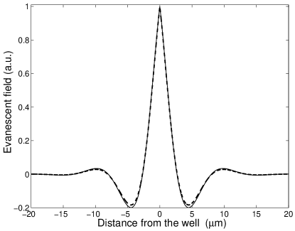
Figure 10: The evanescent light field profile $E=E(z)$ associated with normal (dashed line) and $\gamma_{\rm x}$-induced (solid line) QW polaritons for the strong-weak coupling transition point: $\gamma_{\rm x}=\gamma_{\rm x}^{\rm tr}$ and $k_{\parallel}=k_{\parallel}^{\rm tr}$.

The transition between the strong and weak coupling regimes can also be seen in photoluminescence of the QW radiative states at grazing angles $\phi$ along the structure ($\phi\leqslant 2^{\circ}-5^{\circ}$ for GaAs QWs). The spectral function of the PL signal is

$$S_{\rm PL}=S_{\rm PL}(\omega,\phi)={1\over\pi}\,\frac{\varphi^{\rm x}(k_{\parallel})\mbox{Im}[\omega(k_{\parallel})]}{\big{[}\mbox{Im}[\omega(k_{\parallel})]\big{]}^{2}+\big{[}\omega-\mbox{Re}[\omega(k_{\parallel})]\big{]}^{2}}\ ,$$ (28)

where $\omega(k_{\parallel})$ is the relevant complex solution of Eq. (5) and $\varphi^{\rm x}(k_{\parallel})=\big{|}\mbox{Res}[G_{k_{\parallel}}(\omega);\omega(k_{\parallel})]\big{|}$ is the exciton component of the radiative states, both evaluated at $k_{\parallel}=\big{[}(\omega\sqrt{\varepsilon_{\rm{b}}})/(\hbar c)\big{]}\!\cos\phi$ for real frequency $\omega$. Here, the exciton Green function, as a solution of Eq. (3), is given by

$$G_{\textbf{{k}}_{\parallel}}(\omega)=\frac{2\omega_{\textbf{{k}}_{\parallel}}^{\rm x}}{\omega^{2}-(\omega_{\textbf{{k}}_{\parallel}}^{\rm x})^{2}+(\omega^{2}\varepsilon_{\rm{b}}R_{\rm QW})/(c^{2}\hbar^{2}\kappa)}\ .$$ (29)

The photoluminescence signal at grazing angles is proportional to the spectral function, $I_{\rm PL}\propto S_{\rm PL}(\omega,\phi)$, provided that the radiative states in the vicinity of $k_{\parallel}=k_{0}$ are equally populated.

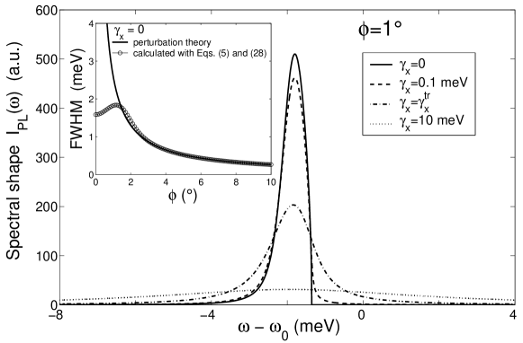
Figure 11: The spectral shape of photoluminescence from the radiative states of QW excitons, $I_{\rm PL}\propto S_{\rm PL}(\omega,\phi)$, calculated with Eq. (28) for the grazing angle $\phi=1^{\circ}$ along a GaAs singe quantum well of 25 nm thickness: $\gamma_{\rm x}=0$ (solid line), 0.1 meV (dashed line), $\gamma_{\rm x}^{\rm tr}=2.4$ meV (dash-dotted line), and 10 meV (dotted line). Inset: The radiative width $\Gamma_{\rm T}$ against angle $\phi$, evaluated with perturbation theory, by using Eq. (6) (dashed line), and calculated with Eqs. (5) and (28) (solid line).

The spectral function $S_{\rm PL}=S_{\rm PL}(\omega)$ is plotted in Fig. 11 for the grazing angle $\phi=1^{\circ}$ and various rates $\gamma_{\rm x}$ of incoherent scattering. For $\gamma_{\rm x}=0$, the spectral function has a well-developed asymmetric shape: $S_{\rm PL}(\omega)=0$ for $\omega\geqslant\omega_{0}+\Delta_{\rm T}^{\rm(B)}$, where the Lamb shift $\Delta_{\rm T}^{\rm(B)}$ is given by Eq. (8) (see also Figs. 2 and 8), $S_{\rm PL}(\omega)$ rises very sharply with decreasing $\omega$ right below $\omega_{0}+\Delta_{\rm T}^{\rm(B)}$, and has a Lorentzian-like red-side tail at $\omega<\omega_{0}$ (see the solid line in Fig. 11). With increasing $\gamma_{\rm x}$ the spectral function $S_{\rm PL}(\omega)$ becomes more broad and symmetric, and finally becomes Lorentzian-shaped at $\gamma_{\rm x}\simeq\gamma_{\rm x}^{\rm tr}$ (see the dotted line in Fig. 11). The red shift of the maximum of $S_{\rm PL}(\omega)$ with increasing $\gamma_{\rm x}$ is consistent with the dependence of the radiative corrections, $\Gamma_{\rm T}$ and $\Delta_{\rm T}$, on $\gamma_{\rm x}$ (see Fig. 8). In order to complete the description, in the inset of Fig. 11 we plot the the radiative width at grazing angles, $\Gamma_{\rm T}=\Gamma_{\rm T}(\phi)$, calculated for $\gamma_{\rm x}=0$ by using standard perturbation theory (dashed line) and evaluated with Eqs. (28)-(29) as the full width at half maximum (FWHM) of the spectral function $S_{\rm PL}=S_{\rm PL}(\omega,\phi)$ (solid line). In the former case the PL signal from the radiative states diverges with $\phi\rightarrow 0$, as $I_{\rm PL}(\phi)\propto\Gamma_{\rm T}(\phi)=\Gamma_{0}/\sin\phi$, while the latter description yields removal of the divergence. The described above $\gamma_{\rm x}$-induced change of the spectral shape of the photoluminescence signal from the radiative states can be seen at lager grazing angles, if, e.g., ZnSe, CdTe, or GaN single QWs with a stronger oscillator strength of exciton-photon interaction are used.

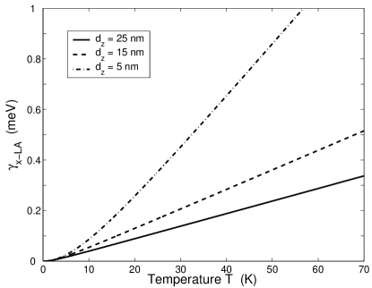
Figure 12: The width $\gamma_{\rm x-LA}=\gamma_{\rm x-LA}(T)$ evaluated for GaAs single QWs of the thickness $d_{z}=25$ nm (solid line), 15 nm (dashed line), and 5 nm (dash-dotted line). Numerical calculations refer to the deformation potential of exciton – LA phonon interaction $D_{\rm DP}=16.1$ eV and the in-plane translational mass $M_{\rm x}=0.4\,m_{0}$ ($m_{0}$ is the free electron mass).

The main mechanisms of incoherent scattering of QW excitons at low temperatures are the deformation potential (DP) interaction of the particles with bulk longitudinal (LA) phonons and exciton-exciton interaction, so that $\gamma_{\rm x}=\gamma_{\rm x-LA}+\gamma_{\rm x-x}$. In order to get an insight of how strong is the first scattering channel, in Fig. 12 we plot $\gamma_{\rm x-LA}$ against temperature $T$ for three values of the thickness of a GaAs single quantum well, $d_{z}=25$ nm, 15 nm, and 5 nm. The dependence $\gamma_{\rm x-LA}=\gamma_{\rm x-LA}(T,d_{z})$, which is calculated by using a method developed in Ref. [Stenius, ], reflects the relaxation of the momentum conservation in the $z$-direction for the QW exciton – bulk LA phonon scattering process. For a low-density, classical gas of QW excitons, when the bath temperature $T$ is much higher than the degeneracy temperature $T_{0}$, the efficiency of QW exciton – QW exciton scattering is evaluated as

$$\gamma_{\rm x-x}={\pi\over 4}\left(\frac{M_{\rm x}}{\mu_{\rm x}}\right)^{2}k_{\rm B}T_{0}\ ,$$ (30)

where $\mu_{\rm x}$ is the reduced mass of a QW exciton, $k_{\rm B}T_{0}=(\pi/2)(\hbar^{2}/M_{\rm x})n_{\rm 2d}$, $n_{\rm 2d}$ is the density of QW excitons, and the spin degeneracy factor of the exciton states is $g=4$. According to Eq. (30), $\gamma_{\rm x-x}$ is proportional to the concentration $n_{\rm 2d}$ of QW excitons, but, as a signature of the quasi-two-dimensionality of the system, the QW exciton – QW exciton scattering rate is independent of the scattering length and temperature $T$ (the latter is valid only for $T\gg T_{0}$). For $n_{\rm 2d}=10^{9}$ cm^-2 and $M_{\rm x}=0.4\,m_{0}$, the degeneracy temperature $T_{0}\simeq 35$ mK, and Eq. (30) yields $\gamma_{\rm x-x}\simeq 0.12$ meV. Figure 12 and estimates with Eq. (30) clearly show that the majority of optical experiments Deveaud1 ; Gurioli ; Eccleston ; Martinez ; Vinattieri ; Wu ; Szczytko ; Deveaud2 with GaAs QWs are undertaken under conditions when the incoherent scattering rate $\gamma_{\rm x}$ can easily achieve the values of $\gamma_{\rm x}^{\rm tr}$ or ${\tilde{\gamma}}_{\rm x}^{\rm tr}$.

Another important question is to what extent the presented model and results are robust against inhomogeneous broadening which is practically inevitable in QW structures. To evaluate the influence of the inhomogeneous broadening, we have examined our model in the paradigm of a “mean-field” QW disorder, developed in Ref. [Andreanie, ]: the results are valid provided that the radiative corrections, $\Gamma_{\rm T}$ and $\Delta_{\rm T}$, are much larger than the inhomogeneous broadening width, $\delta_{\rm inhom}$. Because the radiative corrections relevant to the strong-weak coupling transition refer to the in-plane wavevector $k_{\parallel}\simeq k_{0}$, they are large enough, $\Gamma_{\rm T}\sim\Delta_{\rm T}\sim\big{(}\Gamma_{0}^{2}\omega_{0}\big{)}^{1/3}\sim 1$ meV, to meet the condition $\Gamma_{\rm T},\Delta_{\rm T}\gg\delta_{\rm inhom}$ for nowadays high-quality GaAs single QWs.

VII Conclusions

In this paper we have studied how the $s$-polarized QW polariton states, both confined and radiative, evolve in high-quality (GaAs/AlGaAs) quantum wells with changing incoherent homogeneous broadening $\gamma_{\rm x}$. The transition between the strong and weak coupling regimes of the resonant QW exciton – bulk photon interaction is found and quantified. The following conclusions summarize our results.

(i) In contrast with perturbation theory, there is no divergence of the radiative width $\Gamma=\Gamma_{\rm T}(k_{\|})$ for $k_{\|}\rightarrow k_{0}$. Furthermore, the radiative states of $Y$-mode QW polaritons persist even beyond $k_{0}$, the crossover point of the dispersions of bulk photons and QW excitons. The regularization of the radiative corrections at $k_{\|}=k_{0}$ scales by the energy parameter $\big{(}\Gamma_{0}^{2}\omega_{0}\big{)}^{1/3}\gg\Gamma_{0}$, so that for $\Gamma_{0}=45.5\,\mu$eV used in our numerical evaluations the maximum values of the radiative corrections at $k_{\|}\simeq k_{0}$ are given by $\Gamma_{\rm T}^{\rm max}/2\simeq 0.63$ meV and $\Delta_{\rm T}^{\rm max}\simeq 0.92$ meV.

(ii) For confined QW polaritons, a second, anomalous, $\gamma_{\rm x}$-induced dispersion branch arises and develops with increasing incoherent damping rate $\gamma_{\rm x}$. Such damping-induced dispersion branches are known in plasma physics and in physics of surface electromagnetic waves. In particular, for quasi-particle solution $\omega=\omega(k_{\parallel})$ ($k_{\parallel}$ is real) the critical value of $\gamma_{\rm x}$ for the appearance of the second dispersion branch $\omega=\omega_{2}(k_{\parallel})$ is $\gamma_{\rm x}=\gamma_{\rm c}^{(1)}=\Gamma_{0}$. In this case, i.e., for $\gamma_{\rm x}\geq\gamma_{\rm c}^{(1)}$, a finite sector of the dispersion branch $\omega=\omega_{2}(k_{\|})$ penetrates into the physical part (Re[$\kappa]\geq 0$ and Im[$\omega]\leq 0$) of 3D space $\{k_{\|},\mbox{Im}[\omega],\mbox{Re}[\omega]\}$ from its unphysical area.

(iii) The transition between the strong and weak coupling regimes of the resonant QW exciton – bulk photon interaction is attributed to the incoherent scattering rate, $\gamma_{\rm x}=\gamma_{\rm x}^{\rm tr}$ or $\tilde{\gamma}_{\rm x}^{\rm tr}$, when intersection of the normal and damping-induced dispersion branches of confined $s$-polarized QW polaritons occurs either in $\{k_{\|},\mbox{Im}[\omega],\mbox{Re}[\omega]\}$ coordinate space ($k_{\parallel}$ is real, the quasi-particle solution) or in $\{\omega,\mbox{Im}[k_{\parallel}],\mbox{Re}[k_{\parallel}]\}$ coordinate space ($\omega$ is real, the forced-harmonic solution), respectively. For the quasi-particle solution $\omega=\omega(k_{\parallel})$, the transition damping rate is $\gamma_{\rm x}^{\rm tr}=\gamma_{\rm c}^{(2)}\simeq 1.64\big{(}\Gamma_{0}^{2}\omega_{0}\big{)}^{1/3}$, and the transition point is characterized by Eqs. (15)-(16). For the forced-harmonic solution $k_{\parallel}=k_{\parallel}(\omega)$ ($\omega$ is real), one has $\gamma^{\rm tr}_{\rm x}=$${\tilde{\gamma}}_{\rm c}^{(2)}$$\simeq 1.59\big{[}(\omega_{0}\varepsilon_{\rm{b}})/(M_{\rm x}c^{2})\big{]}^{1/3}\big{(}\Gamma_{0}^{2}\omega_{0}\big{)}^{1/3}$, and the transition point is specified by Eq. (21). Thus for a GaAs single quantum well with the intrinsic radiative lifetime of QW excitons $\tau_{\rm R}=14.5$ ps ($\Gamma_{0}=45.5\,\mu$eV) the transition rates (widths) are given by $\gamma_{\rm x}^{\rm tr}\simeq 2.39$ meV and ${\tilde{\gamma}}_{\rm x}^{\rm tr}\simeq 120\,\mu$eV, respectively.

(iv) For confined QW polaritons, the evanescent light field associated with normal-branch and $\gamma_{\rm x}$-induced-branch polaritons as well as the transition between the strong and weak coupling regimes can be visualized, e.g., by using near-field optical spectroscopy, for both, quasi-particle and forced-harmonic cases. For the radiative states of QW excitons, i.e., for radiative QW polaritons, the transition (the quasi-particle case) can be seen, e.g., in photoluminescence at grazing angles $\phi$, as a qualitative change of the PL spectrum $I_{\rm PL}=I_{\rm PL}(\omega,\phi)$ at a given $\phi$.

VIII ACKNOWLEDGMENTS

We appreciate valuable discussions with K. Cho, S. Elliott, L. Mouchliadis, N. I. Nikolaev, and I. Smolyarenko. Support of this work by the EU RTN Project HPRN-CT-2002-00298 “Photon-mediated phenomena in semiconductor nanostructures” is gratefully acknowledged.

References

- (1) V. M. Agranovich and O. A. Dubovskii, Pis’ma Zh. Teor. Fiz. 3, 345 (1966) [JETP Lett. 3, 223 (1966)].
- (2) M. Nakayama, Solid State Commun. 55, 1053 (1985).
- (3) M. Nakayama and M. Matsuura, Surf. Sci. 170, 641 (1986).
- (4) L. C. Andreani and F. Bassani, Phys. Rev. B 41, 7536 (1990).
- (5) F. Tassone, F. Bassani, and L. C. Andreani, Nuovo Cimento D 12, 1673 (1990); Phys. Rev. B 45, 6023 (1992).
- (6) E. L. Ivchenko, Fiz. Tverd. Tela 33, 2388 (1991) [Sov. Phys. Solid State 33, 1344 (1991)].
- (7) S. Jorda, U. Rossler, and D. Broido, Phys. Rev. B 48, 1669 (1993).
- (8) A. L. Ivanov, H. Wang, J. Shah, T. C. Damen, L. V. Keldysh, H. Haug, and L. N. Pfeiffer, Phys. Rev. B 56, 3941 (1997).
- (9) A. L. Ivanov, H. Haug, and L. V. Keldysh, Phys. Reports 296, 237 (1998).
- (10) A. L. Ivanov, P. Borri, W. Langbein, and U. Woggon, Phys. Rev. B 69, 075312 (2004).
- (11) M. Orrit, C. Aslangul, and P. Kottis, Phys. Rev. B 25, 7263 (1982).
- (12) E. Hanamura, Phys. Rev. B 38, 1228 (1988).
- (13) L. C. Andreani, F. Tassone, and F. Bassani, Solid State Commun. 77, 641 (1991).
- (14) D. Citrin, Phys. Rev. B 47, 3832 (1993).
- (15) J. Feldmann, G. Peter, E. O. Göbel, P. Dawson, K. Moore, C. Foxon, and R. J. Elliott, Phys. Rev. Lett. 59, 2337 (1987).
- (16) B. Deveaud, F. Clérot, N. Roy, K. Satzke, B. Sermage, and D. S. Katzer, Phys. Rev. Lett. 67, 2355 (1991).
- (17) M. Gurioli, A. Vinattieri, M. Colocci, C. Deparis, J. Massies, G. Neu, A. Bosacchi, and S. Franchi, Phys. Rev. B 44, 3115 (1991).
- (18) R. Eccleston, B. F. Feuerbacher, J. Kuhl, W. W. Rühle, and K. Ploog, Phys. Rev. B 45, 11403 (1992).
- (19) J. Martinez-Pastor, A. Vinattieri, L. Carraresi, M. Colocci, Ph. Roussignol, and G. Weimann, Phys. Rev. B 47, 10456 (1993).
- (20) A. Vinattieri, J. Shah, T. C. Damen, D. S. Kim, L. N. Pfeiffer, M. Z. Maialle, and L.J. Sham, Phys. Rev. B 50, 10868 (1994).
- (21) J. Szczytko, L. Kappei, J. Berney, F. Morier-Genoud, M. T. Portella-Oberli, and B. Deveaud, Phys. Rev. Lett. 93, 137401 (2004).
- (22) B. Deveaud, J. Szczytko, L. Kappei, J. Berney, F. Morier-Genoud, and M. Portella-Oberli, phys. stat. sol. (c) 2, 2947 (2005).
- (23) N. Moret, D. Y. Oberli, E. Pelucchi, N. Gogneau, A. Rudra, and E. Kapon, Appl. Phys. Lett. 88, 141917 (2006).
- (24) M. Kohl, D. Heitmann, P. Grambow, and K. Ploog, Phys. Rev. B 37, 10927 (1988); 42, 2941 (1990).
- (25) J. Lagois and B. Fisher, in Surface Polaritons, edited by V. M. Agranovich and A. A. Maradudin, Vol. 1 of Modern Problems in Condensed Matter Sciences (North-Holland, Amsterdam 1982), Chap. 2.
- (26) H. F. Hess, E. Betzig, T. D. Harris, L. N. Pfeiffer, and K. W. West, Science 264, 1740 (1994).
- (27) Q. Wu, R. D. Grober, D. Gammon, and D. S. Katzer, Phys. Rev. Lett. 83, 2652 (1999).
- (28) F. Pulizzi, P. C. M. Christianen, J. C. Maan, S. Eshlaghi, D. Reuter, and A. D. Wieck, phys. stat. sol. (a) 190, 641 (2002).
- (29) W. C. Tait, Phys. Rev. B 5, 648 (1972).
- (30) G. Battaglia, A. Quattropani, and P. Schwendimann, Phys. Rev. B 34, 8258 (1986).
- (31) N. I. Nikolaev, A. Smith, and A. L. Ivanov, J. Phys.: Condens. Matter 16, S3703 (2004).
- (32) J. J. Hopfield, Phys. Rev. 112, 1555 (1958).
- (33) V. M. Agranovich and V. L. Ginzburg, Crystal Optics with Spatial Dispersion and Excitons, 2nd ed. (Springer, New York, 1984).
- (34) S. Jorda, Phys. Rev. B 50, 2283 (1994).
- (35) V. V. Popov, T. V. Teperik, N. J. M. Horing, and T. Yu. Bagaeva, Solid State Commun. 127, 589 (2003).
- (36) L. D. Landau and E. M. Lifshitz, Quantum Mechanics, Course of Theoretical Physics, Volume III (Pergamon Press, Oxford, 1981), 128.
- (37) Yu. M. Aliev, H. Schlüter, and A. Shivarova, Guided-Wave-Produced Plasmas (Springe-Verlag, Berlin, 2000), Chap. 3.
- (38) P. Halevi, Electromagnetic Surface Modes (Wiley, Chichester, 1982).
- (39) P. Halevi, Phys. Rev. B 12, 4032 (1975).
- (40) R. Loudon, J. Phys. A 3, 233 (1970).
- (41) L. C. Andreani, G. Panzarini, A. V. Kavokin, and M. R. Vladimirova, Phys. Rev. B 57, 4670 (1998).
- (42) D. S. Citrin and T. D. Backes, phys. stat. sol. (b) 243, 2349 (2006).
- (43) G. W. Farnell, in Acoustic Surface Waves, edited by A. Oliner, Topics in Applied Physics Vol. 24 (Springer, Berlin, 1978).
- (44) P. Stenius and A. L. Ivanov, Solid State Commun. 108, 117 (1998).