Peierls ground state and excitations in the electron-lattice correlated system (EDO-TTF)₂X

Abstract

We investigate the exotic Peierls state in the one-dimensional organic compound (EDO-TTF)₂X, wherein the Peierls transition is accompanied by the bending of molecules and also by a fourfold periodic array of charge disproportionation along the one-dimensional chain. Such a Peierls state, wherein the interplay between the electron correlation and the electron-phonon interaction takes an important role, is examined based on an extended Peierls$-$Holstein$-$Hubbard model that includes the alternation of the elastic energies for both the lattice distortion and the molecular deformation. The model reproduces the experimentally observed pattern of the charge disproportionation and there exists a metastable state wherein the energy takes a local minimum with respect to the lattice distortion and/or molecular deformation. Furthermore, we investigate the excited states for both the Peierls ground state and the metastable state by considering the soliton formation of electrons. It is shown that the soliton excitation from the metastable state costs energy that is much smaller than that of the Peierls state, where the former is followed only by the charge degree of freedom and the latter is followed by that of spin and charge. Based on these results, we discuss the exotic photoinduced phase found in (EDO-TTF)₂PF₆.

I Introduction

The quasi-one-dimensional molecular compound, (EDO-TTF)₂PF₆, (Refs. Chollet2005, ; Onda2005, ; Koshihara2006, ; Ota2002, ; Drozdova2004, ) (where EDO-TTF denotes ethylenedioxytetrathiafulvalene) has been studied as one of the central topics showing a photoinduced phase transition. Tokura2006 The 1/4-filled (EDO-TTF)₂PF₆ system exhibits a Peierls insulating state, which is accompanied by a charge disproportionation and the bending of the EDO-TTF molecules.Ota2002 Several experiments indicate that this Peierls transition comes from the cooperation effect of the molecular deformation, charge ordering, and anion ordering. The charge disproportionation along the one-dimensional chain exhibits a fourfold periodicity given by a periodic array of [0, 1, 1, 0]; i.e., the pattern is an alternation of two charge-rich sites and two charge-poor sites. A remarkable feature of the insulating state is the large bending of the EDO-TTF molecules, which does exist even for the neutral single molecule. The degree of bending depends on the valence of the EDO-TTF molecule. Each molecule in the high-temperature metallic phase has a valence of $+0.5$, while the valences in the insulating state are estimated as $+0.9$ and $+0.1$ for hole-rich and hole-poor sites, respectively. Drozdova2004 In the insulating state, the degree of bending is enhanced at the electron-rich site and is suppressed at the electron-poor site; i.e., the bending (flattening) of the molecule is observed in the electron-rich (-poor) site. However, the mechanism beyond the kinetic-energy gain is required in order to explain the bending and/or flattening of the molecules.

Recent experimental studies have focused on the phase transition induced by a weak laser pulse; i.e., the photoinduced phase transition, and suggest that (EDO-TTF)₂PF₆ exhibits a gigantic photoresponse in the low-temperature phase.Chollet2005 In the photoinduced phase, the lattice distortion and the molecular deformation are relaxed and the system shows a metallic behavior. In addition, it has been discussed that the photoinduced phase shows an exotic behavior, and is different from that in the high-temperature metal phase. Onda2005 From these experiments, it has been argued that a new phase, which is not possible as a ground state and is related to a metastable state, is achieved by the photoexcitation. Therefore it is of particular interest to investigate the mechanism of a metallic behavior in such a metastable state, which may be related to the electronic correlation.

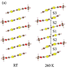
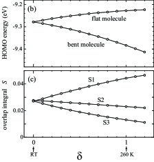
Figure 1: (Color online) (a) Crystal structure of (EDO-TTF)₂PF₆ at RT and 260 K. (b) The HOMO energy level of the EDO-TTF molecules as a function of the distortion parameter $\delta$ (see text). $\delta=0$ corresponds to the case at RT and $\delta=1$ to that at 260 K. (c) The overlap integral as a function of $\delta$. At RT, all molecules are equivalent and S1$=$S3, while S1$\neq$S2.

A theoretical investigation on the Peierls state in the one-dimensional (1D) quarter-filled system has been performed based on the Peierls$-$Hubbard model including the effect of the onsite Coulomb repulsion $U$ and the intersite one $V$. Ung ; Clay ; Kuwabara2003 ; Seo2007JPSJ It has been clarified that the spatial variation of the conventional charge-density wave at the quarter-filled system is of the site-centered type; i.e., the charge density takes a maximum at a site. On the other hand, in the Peierls state of (EDO-TTF)₂PF₆, it takes a maximum at the location between two neighboring sites; i.e., it is of the bond-centered type. It has been shown, within the mean-field theory, that the experimentally observed pattern of charge disproportionation can be reproduced by taking into account the alternation of the elastic energies.Omori2007 It has also been shown that, due to the effect of the elastic-energy modulation, the Peierls state and the charge-ordered (CO) state with a twofold periodicity compete with each other, and there exists the metastable state wherein the energy takes a local minimum with respect to the lattice distortion. Omori2007 The trigger of such a metastable state comes from the competition between the electron correlation and the electron-phonon interaction. The former favors the CO state with a twofold periodicity, while the latter supports the charge disproportionation with a fourfold periodicity. In the present paper, we study both the Peierls ground state and the metastable state, in terms of the phase representation based on bosonization. Furthermore, we also examine the two kinds of excitations: (i) the excitation followed by the lattice relaxation and (ii) the purely electronic excitations. In §2, our model consisting of an electron-lattice system is given and a representation based on bosonization is introduced. The Peierls distortion with the bond order is taken by considering the alternation of the elastic constant for the lattice distortion. In §3, the ground state is analyzed in terms of the phase variables of spin and charge to show the condition for the existence of the metastable state. Using an extended Peierls$-$Holstein$-$Hubbard model treated in terms of the bosonization method, we demonstrate how the first-order transition occurs where the result is qualitative the same as the previous mean-field result.Omori2007 In §4, the excitations from both the Peierls state and the metastable state are examined by calculating the soliton formation energy. It is shown that the latter is much smaller than that of the former. Section V is devoted to the summary and discussions.

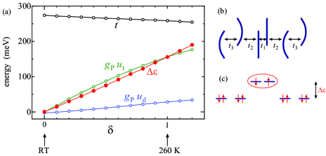
Figure 2: (Color online) (a) The HOMO energy difference $\Delta\varepsilon$ and the magnitude of lattice tetramerization and dimerization as a function of the distortion parameter $\delta$. (b) Schematic view of crystal structure of (EDO-TTF)₂PF₆ at 260 K and (c) the corresponding energy diagram, where $\Delta\varepsilon=156$ meV, $t_{1}=443$ meV, $t_{2}=230$ meV, and $t_{3}=131$ meV.

II Model for the EDO-TTF compound

As a system exhibiting the correlated Peierls state, we consider a tight-binding Hubbard model coupled with lattice distortion and molecular deformation, through the electron-phonon interaction. In this section, by focusing on the Peierls state in (EDO-TTF)₂PF₆, we first examine the characteristic features of the molecular deformation and the lattice distortion of the EDO-TTF molecules, based on a quantum-chemical calculation. Next, we derive the model Hamiltonian of the 1D quarter-filled Peierls$-$Holstein$-$Hubbard model, and we introduce the “phases” of the lattice distortion and of the molecular deformation.

II.1 Molecular deformation in (EDO-TTF)₂PF₆

It has been confirmed that (EDO-TTF)₂PF₆ exhibits a first-order transition at around 280 K. Ota2002 The overlap integrals at room temperature (RT) and at 260 K have been estimated by an extended Hückel calculationMori_extdh based on an x-ray structure analysis. At room temperature, there is a very weak dimerization and the overlap integral is almost uniform along the stacking direction. However, at 260 K, there is a strong variation among the overlap integrals, given by $S1$, $S2$, and $S3$, along the stacking direction. Ota2002

In order to make the situation clearer, we estimate the energy levels of the highest occupied molecular orbitals (HOMOs) for the flat and bent molecules, and also estimate the overlap integrals, as a function of the lattice distortion and/or molecular deformation. Here we simply perform the interpolation of the coordinates for the respective atoms in the EDO-TTF molecules between RT and 260 K by using the relation $(x,y,z)=(x,y,z)_{\mathrm{RT}}+(\Delta x,\Delta y,\Delta z)\delta$, where $\delta$ is the distortion parameter and $(\Delta x,\Delta y,\Delta z)\equiv(x,y,z)_{\mathrm{260\,\,K}}-(x,y,z)_{\mathrm{RT}}$. For both cases of RT and 260 K, the $y$ axis is chosen along the stacking direction [the vertical axis in Fig. 1(a)] and the $x$ axis is set to the projection of the molecular-long direction to perpendicular to $y$ [the horizontal axis in Fig. 1(a)]. At $\delta=0$ $(1)$, the atomic coordinates at RT (260 K) are reproduced. Using this relation and the extended Hückel method, Mori_extdh we examine the $\delta$ dependence of the HOMO energy levels [Fig. 1(b)] and the overlap integral [Fig. 1(c)]. Here we neglect the flipping disorder of the terminal ethylene group Ota2002 and use only the coordinates of the atoms with a high occupation rate. We found that the HOMO energy level for the bent EDO-TTF molecule is sufficiently lowered due to the molecular deformation, and that the overlap integrals do not change their sign as a function of $\delta$. We estimate the transfer integrals from the overlap integrals by using the empirical relation $t_{i}=S_{i}\times$ 10 eV.Mori_extdh At 260 K, the transfer integrals are estimated as $t_{1}=442$ meV, $t_{2}=230$ meV, and $t_{3}=131$ meV. A notable feature of this compound is that the electron-rich EDO-TTF molecule tends to bend and the hole-rich EDO-TTF molecule tends to be flat [Figs. 2(b) and 2(c)], Ota2002 where the valence of the former (latter) is 0.1 (+0.9). The energy level of the HOMO is $\epsilon_{F}=-9.222$ eV for the flat EDO-TTF molecule, while $\epsilon_{B}=-9.442$ eV for the bent molecule. This lattice distortion pattern shows a strong tetramerization $u_{t}$ in addition to the lattice dimerization $u_{d}$, which are estimated from

$$t_{1} = t+g_{P}u_{t}+g_{P}u_{d},$$ (1a)

$$t_{2} = t-g_{P}u_{d},$$ (1b)

$$t_{3} = t-g_{P}u_{t}+g_{P}u_{d},$$ (1c)

where $g_{P}$ is the electron-phonon coupling constant. The lattice distortion parameter $u_{t}$ characterizes a modulation of fourfold periodicity; i.e., the lattice tetramerization, and the parameter $u_{d}$ characterizes a modulation of twofold periodicity; i.e., the lattice dimerization. It can be found that the strength of the lattice tetramerization is $g_{P}u_{t}=156$ meV, while that of the lattice dimerization is $g_{P}u_{d}=29$ meV.

We note that the spatial variation of the lattice distortion corresponds to neither the conventional $2k_{F}$ charge-density waveUng ; Clay state nor the dimer-Mott+spin-Peierls (SP) state,Kuwabara2003 ; Seo2007JPSJ in which the lattice tetramerization takes a maximum at $t_{1}$ (i.e., $g_{P}u_{t}>0$), and the lattice dimerization has a maximum at $t_{2}$ (i.e., $g_{P}u_{d}<0$). In the dimer-Mott+SP state, which occurs in the presence of the lattice dimerization, the system becomes effectively half filling and each electron is localized at the location of each lattice dimer. When the $2k_{F}$ Peierls instability is taken into account, such a paramagnetic insulator changes into the non-magnetic SP state. Kuwabara2003 ; Seo2007JPSJ Then, one finds $g_{P}u_{t}>0$ and $g_{P}u_{d}<0$ in the dimer-Mott + SP state. However, in the case of (EDO-TTF)₂PF₆, both the lattice tetramerization and the lattice dimerization take the maximum at $t_{1}$ (i.e., $g_{P}u_{t}>0$ and $g_{P}u_{d}>0$). This lattice distortion pattern in (EDO-TTF)₂PF₆ is qualitatively different from that in the dimer-Mott + SP state and has not been discovered in previous theoretical studies. In this sense, the Peierls ground state of (EDO-TTF)₂PF₆ is quite exotic and, is examined, in the present paper, by constructing a model that can reproduce such a ground state.

II.2 Model Hamiltonian

Based on the above consideration, we introduce a 1D extended Hubbard model coupled with the lattice through the electron-phonon interaction. Since there are two molecules within the unit cell, we introduce two sites referred to $l=1$ and $l=2$. In this study, we are based on the hole picture; i.e., there is one carrier per two sites. Our Hamiltonian is given by

$$H=H_{\mathrm{e}}+H_{\mathrm{e\mbox{-}ph}}+H_{\mathrm{ph}},$$ (2)

where the purely electronic part $H_{\mathrm{e}}$ is ($j=1,\ldots,N$)

$$H_{\mathrm{e}} = -t\sum_{j,s}\left(c_{j,1,s}^{\dagger}c_{j,2,s}+\mathrm{H.c.}\right)$$

$${}-t\sum_{j,s}\left(c_{j,2,s}^{\dagger}c_{j+1,1,s}+\mathrm{H.c.}\right)$$

$${}+U\sum_{j}(n_{j,1,\uparrow}n_{j,1,\downarrow}+n_{j,2,\uparrow}n_{j,2,\downarrow})$$

$${}+V\sum_{j}(n_{j,1}n_{j,2}+n_{j,2}n_{j+1,1})-\mu\sum_{j,l(=1,2)}n_{j,l},$$

the electron-phonon coupling term $$H_{\mathrm{e\mbox{-}ph}}$$ is

$$H_{\mathrm{e\mbox{-}ph}} = \sum_{j,s}g_{P}(u_{j,1}-u_{j,2})\left(c_{j,1,s}^{\dagger}c_{j,2,s}+\mathrm{H.c.}\right)$$ (3b)

$${}+\sum_{j,s}g_{P}(u_{j,2}-u_{j+1,1})\left(c_{j,2,s}^{\dagger}c_{j+1,1,s}+\mathrm{H.c.}\right)$$

$${}+\sum_{j,l(=1,2)}g_{\mathrm{H}}v_{j,l}\left(n_{j,l}-\frac{1}{2}\right),$$

and the phonon term $$H_{\mathrm{ph}}$$ is

$$H_{\mathrm{ph}} = \frac{K_{P}}{2}\sum_{j}\left[(u_{j,1}-u_{j,2})^{2}+(u_{j,2}-u_{j+1,1})^{2}\right]$$ (3c)

$${}+\frac{K_{H}}{2}\sum_{j}(v_{j,1}^{2}+v_{j,2}^{2})$$

$${}+\sum_{j}F(u_{j,1},u_{j,2},v_{j,1},v_{j,2}).$$

The parameter $v_{j,l}$ represents the degree of molecular deformation wherein the shape of the molecule depends on its sign; i.e., the molecule is bent for $v_{j,l}>0$, while the molecule is flat for $v_{j,l}<0$. In Eq. (LABEL:eq:He), $c_{j,l,s}$ denotes the annihilation operator of an electron with spin $s(=\uparrow,\downarrow)$ at the $l$th site within the $j$th unit cell, and $n_{j,l,s}=c_{j,l,s}^{\dagger}c_{j,l,s}$, where $t$ is the transfer energy and $\mu$ is the chemical potential. The parameters $U(>0)$ and $V(>0)$ denote the magnitudes for the on-site and nearest neighbor interactions. In Eq. (3b), $g_{H}$ is the electron-phonon coupling constant of the on-site (Holstein) type, and the Peierls-type electron-phonon coupling constant is given by $g_{P}$. In Eq. (3c), the parameters $K_{H}$ and $K_{P}$ are the conventional elastic constant for the molecular deformation and the lattice distortion, respectively. The quantity $F(u_{j,1},u_{j,2},v_{j,1},v_{j,2})$ represents the specific features in (EDO-TTF)₂PF₆, which will be defined in Sec. II C.

Here, we note that the present Hamiltonian can reasonably account for the relation between the valence of the molecule and the molecular deformation $v_{j,l}$. For simplicity, we consider the case of the single molecule, wherein the Hamiltonian is given by

$$H_{1}=g_{H}v\left(n-\frac{1}{2}\right)+\frac{1}{2}K_{H}v^{2}.$$ (4)

By minimizing $H_{1}$ with respect to $v$, we find that the lattice distortion depends on the charge on the molecule, e.g.,

$$v=\left\{\begin{array}[]{ll}\displaystyle+\frac{g_{H}}{2K_{H}}&\mbox{for }n=0\\ \\ \displaystyle-\frac{g_{H}}{2K_{H}}&\mbox{for }n=1.\end{array}\right.$$ (8)

Thus, we obtain that the neutral molecule ($n=0$) becomes bent ($v<0$); on the other hand, the ionic molecule ($n=1$) becomes flat ($v>0$).

II.3 Modifications of phonon term $H_{\mathrm{ph}}$

Here we examine the characteristic features of the crystal structure of (EDO-TTF)₂PF₆ [Fig. 1(a)], for the model that reproduces the Peierls ground state. If $F(u_{j,1},u_{j,2},v_{j,1},v_{j,2})=0$ in Eq. (3c), the model reduces to the conventional Peierls$-$Holstein$-$Hubbard model at quarter filling.Ung ; Clay ; Kuwabara2003 ; Seo2007JPSJ Noting two kinds of molecules in the unit cell at the high-temperature phase of the EDO-TTF compounds, we introduce two kinds of elastic constants for the lattice distortion and the molecule deformation, within the unit-cell and between neighboring cells. Such a difference would play important roles on the low-energy properties. We consider the term, $F(u_{j,1},u_{j,2},v_{j,1},v_{j,2})$, given by

$$F(u_{j,1},u_{j,2},v_{j,1},v_{j,2})$$

$$\qquad=-\frac{\delta K_{P}}{4}\sum_{j}\left[(u_{j,1}-u_{j,2})^{2}-(u_{j,2}-u_{j+1,1})^{2}\right]$$

$$\qquad-\frac{\delta K_{H}}{2}\sum_{j}(v_{j,1}+v_{j,2})^{2},$$ (9)

where the $\delta K_{P}$ term comes from the difference between the elastic constants for the lattice distortion, within the unit cell and between neighboring cells. The $\delta K_{H}$ term represents the difference in the energy gain of the two-molecular deformation within the unit cell. The intrinsic property of the bending of the EDO-TTF molecules would play important roles for the lattice distortion, since a pair of two molecules faces each other in the unit cell. Ota2002 In fact, in the ordered phase, one pair of molecules shows strong bending and another pair of the molecules becomes more flat [Fig. 1(a)]. Such an effect due to the pairing of the EDO-TTF molecules can be taken into account in our model by considering the additional terms of Eq. (9).

From the mean-field approach, Omori2007 it has been pointed out that the effect of $\delta K_{P}$ is important to determine the multistable states induced by the lattice distortion. The details of the effects of $\delta K_{P}$ and $\delta K_{H}$ are discussed in Sec. III.

II.4 Lattice distortion and molecular deformation

In general, the lattice distortion $u_{j,l}$ in quarter-filled systems can be decomposed into the component with a twofold periodicity (i.e., dimerization), $u_{d}$, and that with a fourfold periodicity (i.e., tetramerization), $u_{t}$. Clay ; Kuwabara2003 ; Sugiura2003 Even for the freedom of the molecular deformation, $v_{j,l}$, it can be decomposed into the component with a twofold periodicity, $v_{d}$, and that with a fourfold periodicity, $v_{t}$. We introduce these quantities by using the relations:

$$u_{j,1} = +(-1)^{j}\frac{u_{t}}{\sqrt{2}}\cos\xi-\frac{u_{d}}{2},$$ (10a)

$$u_{j,2} = -(-1)^{j}\frac{u_{t}}{\sqrt{2}}\sin\xi+\frac{u_{d}}{2},$$ (10b)

$$v_{j,1} = +(-1)^{j}\frac{v_{t}}{\sqrt{2}}\cos\zeta-\frac{v_{d}}{2},$$ (10c)

$$v_{j,2} = +(-1)^{j}\frac{v_{t}}{\sqrt{2}}\sin\zeta+\frac{v_{d}}{2}.$$ (10d)

The phases $\xi$ and $\zeta$ determine the spatial pattern of the tetramerizations $u_{t}$ and $v_{t}$, respectively.

For the later convenience, we renumber the site index $j$ as $i=2j+(l-1)$; accordingly, we rewrite $c_{j,l,s}\to c_{i,s}$. By using Eq. (10), the Hamiltonian (2) is rewritten as

$$H = -\sum_{i,s}\left[t-g_{P}u_{t}\cos\left(\frac{\pi}{2}i+\xi-\frac{\pi}{4}\right)+(-1)^{i}g_{P}u_{d}\right]$$

$${}\qquad\times\left(c_{i,s}^{\dagger}c_{i+1,s}+\mathrm{H.c.}\right)$$

$${}+\sum_{i}g_{H}\frac{v_{t}}{\sqrt{2}}\cos\left(\frac{\pi}{2}i-\zeta\right)\left(n_{i}-\frac{1}{2}\right)-\mu\sum_{i}n_{i}$$

$${}+U\sum_{i}n_{i,\uparrow}n_{i,\downarrow}+V\sum_{i}n_{i}n_{i+1}$$

$${}+N\frac{K_{P}}{4}u_{t}^{2}-N\frac{\delta K_{P}}{4}u_{t}^{2}\sin 2\xi+N\frac{K_{P}}{2}u_{d}^{2}$$

$${}+N\frac{K_{H}-\delta K_{H}}{4}v_{t}^{2}-N\frac{\delta K_{H}}{4}v_{t}^{2}\sin 2\xi+N\frac{K_{H}}{4}v_{d}^{2}.$$

Now, we specify the phases of $\xi$ and $\zeta$, which reproduce the Peierls state observed in (EDO-TTF)₂PF₆. The crystal structure of (EDO-TTF)₂PF₆ for the metallic state at high temperature shows an alternation of the bending of the molecule, where all of the molecules are identical crystallographically.Ota2002 For the insulating state at low temperature, the neutral molecule exhibits a large bending and the ionic molecule becomes rather flat, where the adjacent two molecules at the neutral sites are oppositely located with the same degree of bending and becomes convex outside. The transfer integral between adjacent bent molecules becomes small while that between adjacent flat molecules becomes large. Such a pattern of the molecular deformation and lattice distortion can be reproduced by setting $\xi=\zeta=\pi/4$. When $\xi=\zeta=\pi/4$, the transfer-energy modulation is given by

$$(t_{3},t_{2},t_{1},t_{2},t_{3},t_{2},t_{1},t_{2}),$$ (12)

for $i=0,1,2,3,4,\ldots$, where $t_{1}$, $t_{2}$, and $t_{3}$ are the same as those given in Eq. (1). The schematic view of the modulation pattern is shown in Fig. 3. The site-energy modulation is given by

$$\frac{1}{2}g_{H}(+v_{t},+v_{t},-v_{t},-v_{t},+v_{t},+v_{t},-v_{t},-v_{t},\cdots),\qquad$$ (13)

for $i=0,1,2,3,4,\ldots$, where the component of the molecular deformation with the twofold periodicity $v_{d}$ vanishes for (EDT-TTF)₂PF₆ (see also Fig. 3).

III Bosonization Representation

Here, we represent the Hamiltonian in terms of bosonic phase variables. Giamarchi_book By setting $a$ as the lattice constant, the electron density operator can be represented as Giamarchi_book

$$\frac{n_{i}}{a} = \frac{1}{4a}+\frac{1}{\pi}\frac{d\phi_{\rho}}{dx}-\frac{2}{\pi a}\sin(2k_{F}x+\phi_{\rho})\cos\phi_{\sigma}$$ (14)

$${}-\frac{2c}{\pi a}\cos(4k_{F}x+2\phi_{\rho}),$$

where $x=ia$ and $c$ is a nonuniversal constant. The Fermi momentum is $k_{F}=\pi/(4a)$. The quantities $\phi_{\rho}$ and $\phi_{\sigma}$ are bosonic phase variables and Eq. (14) is justified by the microscopic representation of the field operator.

Here we briefly recall the relation between the lattice distortion and electron density modulation, based on the phase-variable representation. We tentatively assume $c=0$. If the phases are locked at $(\langle\phi_{\rho}\rangle,\langle\phi_{\sigma}\rangle)=(\pi/4,0)$, the expectation value of the charge-density operator are given by

$$\langle n_{i}\rangle = \frac{1}{4}-\frac{2}{\pi}\sin(2k_{F}x+\pi/4).$$ (15)

The pattern of charge modulation is given by $\langle n_{j}\rangle=(\,\circ\,\circ\,\bigcirc\,\bigcirc\,\circ\,\ldots\,)$ for $j=0,1,2,3,4,\ldots$, which is compatible with the lattice distortion and molecular deformation given in Eqs. (12) and (13). This means that the tetramerization pattern observed in (EDO-TTF)₂PF₆ is reproduced if the phases are locked at $\xi=\zeta=\pi/4$ and $(\langle\phi_{\rho}\rangle,\langle\phi_{\sigma}\rangle)=(\pi/4,0)$.

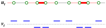
Figure 3: (Color online) The modulation pattern of the transfer integral induced by the lattice distortion $u_{t}$ and that of the onsite energy level induced by the molecular deformation $v_{t}$. In this view, we have considered only the modulations of tetramerization; i.e., of fourfold periodicity.

Based on the phase-variable representation, the bosonized Hamiltonian Fukuyama_review ; Giamarchi_book ; Tsuchiizu2001 is obtained as $H=\int dx\,\mathcal{H}$, where

$$\mathcal{H} = \frac{v_{\rho}}{4\pi}\left[\frac{1}{K_{\rho}}(\partial_{x}\phi_{\rho})^{2}+K_{\rho}(\partial_{x}\theta_{\rho})^{2}\right]+\frac{v_{\sigma}}{4\pi}\left[\frac{1}{K_{\sigma}}(\partial_{x}\phi_{\sigma})^{2}+K_{\rho}(\partial_{x}\theta_{\sigma})^{2}\right]+\frac{g_{1/4}}{2\pi^{2}a^{2}}\cos 4\phi_{\rho}+\frac{g_{\sigma}}{2\pi^{2}a^{2}}\cos 2\phi_{\sigma}$$ (16)

$${}-\frac{2}{\pi a}g_{P}u_{t}\cos\left(\phi_{\rho}-\xi\right)\cos\phi_{\sigma}-\frac{1}{\sqrt{2}\pi a}g_{H}v_{t}\sin\left(\phi_{\rho}+\zeta\right)\cos\phi_{\sigma}+\frac{U}{\pi^{2}ta}g_{P}u_{d}\sin 2\phi_{\rho}+\frac{U}{2\sqrt{2}\pi^{2}ta}g_{H}v_{d}\cos 2\phi_{\rho}$$

$${}+\frac{K_{P}}{4a}u_{t}^{2}-\frac{\delta K_{P}}{8a}u_{t}^{2}\sin 2\xi+\frac{K_{P}}{2a}u_{d}^{2}+\frac{K_{H}-\delta K_{H}}{8a}v_{t}^{2}-\frac{\delta K_{H}}{8a}v_{t}^{2}\sin 2\zeta+\frac{K_{H}}{8a}v_{d}^{2},\qquad$$

In Eq. (16), $\theta_{\nu}$ ($\nu=\rho$ and $\sigma$) is the phase variable which is canonically conjugate to $\phi_{\nu}$ and $[\phi_{\nu}(x),\theta_{\nu}(x^{\prime})]=i\pi\mathrm{sgn}(x-x^{\prime})$. The parameters $v_{\rho}$ and $v_{\sigma}$ are the velocity of the charge and spin excitations, and $K_{\rho}$ and $K_{\sigma}$ are the Tomonaga$-$Luttinger parameters. It is noted that $K_{\rho}<1$ for the repulsive interaction and $K_{\sigma}=1$ for the paramagnetic state. From the perturbative calculation, Tsuchiizu2001 the coupling $g_{1/4}$ is given by $g_{1/4}\propto U^{2}(U-4V)$, where it is noticed that $g_{1/4}$ is positive for small $V$ but becomes negative for large $V$. For small $V$, the phase $\phi_{\rho}$ is locked at $\langle\phi_{\rho}\rangle=\pi/4$(mod $\pi/2$); while for large $V$ the phase is locked at $\langle\phi_{\rho}\rangle=0$(mod $\pi/2$).

In terms of the bosonized Hamiltonian, we examine the effect of additional terms including $\delta K_{P}$ and $\delta K_{H}$. First, we discuss the state in the case of $\delta K_{P}=\delta K_{H}=0$. The locking position of the phases $\xi$ and $\zeta$ is determined by $\phi_{\rho}$; i.e., $\xi=\phi_{\rho}$ and $\zeta=\pi/2-\phi_{\rho}$. Thus, the total Hamiltonian can be expressed as

$$\mathcal{H}|_{\delta K=0} = \frac{v_{\rho}}{4\pi}\left[\frac{1}{K_{\rho}}(\partial_{x}\phi_{\rho})^{2}+K_{\rho}(\partial_{x}\theta_{\rho})^{2}\right]$$ (17)

$${}+\frac{v_{\sigma}}{4\pi}\left[\frac{1}{K_{\sigma}}(\partial_{x}\phi_{\sigma})^{2}+K_{\rho}(\partial_{x}\theta_{\sigma})^{2}\right]$$

$${}+\frac{g_{1/4}}{2\pi^{2}a^{2}}\cos 4\phi_{\rho}+\frac{g_{\sigma}}{2\pi^{2}a^{2}}\cos 2\phi_{\sigma}$$

$${}-\frac{2}{\pi a}g_{P}u_{t}\cos\phi_{\sigma}-\frac{1}{\sqrt{2}\pi a}g_{H}v_{t}\cos\phi_{\sigma}$$

$${}+\frac{U}{\pi^{2}ta}g_{P}u_{d}\sin 2\phi_{\rho}+\frac{U}{2\sqrt{2}\pi^{2}ta}g_{H}v_{d}\cos 2\phi_{\rho}$$

$${}+\frac{K_{P}}{4a}u_{t}^{2}+\frac{K_{P}}{2a}u_{d}^{2}+\frac{K_{H}}{8a}v_{t}^{2}+\frac{K_{H}}{8a}v_{d}^{2},\qquad$$

which can reproduce the previous results (e.g., Fig. 4 in Ref. Clay, ) qualitatively. The undistorted state can be obtained for a small electron-phonon coupling of $g_{P}$ and $g_{H}$. By increasing $g_{P}$ only, we obtain a solution where $u_{d}$ becomes finite and the phases $\phi_{\rho}$ and $\xi$ are locked at $\phi_{\rho}=\xi=\pi/4$(mod $\pi$) (if $u_{d}<0$) or at $\phi_{\rho}=\xi=3\pi/4$(mod $\pi$) (if $u_{d}>0$). This state corresponds to the $4k_{F}$ bond-order wave (BOW) state in Ref. Clay, . By further increasing $g_{P}$, we obtain a state wherein the tetramerizations $u_{t}$ and $v_{t}$ become finite. For $u_{d}<0$, the lattice distortion [Eq. (10)] is given by

$$u_{j,1} = +\frac{|u_{d}|}{2}+(-1)^{j}\frac{u_{t}}{2},$$ (18a)

$$u_{j,2} = -\frac{|u_{d}|}{2}-(-1)^{j}\frac{u_{t}}{2}.$$ (18b)

Then the resultant hopping integrals are given by

$$t_{1} = t-g_{P}|u_{d}|+g_{P}u_{t},$$ (19a)

$$t_{2} = t+g_{P}|u_{d}|,$$ (19b)

$$t_{3} = t-g_{P}|u_{d}|-g_{P}u_{t}.$$ (19c)

where $t_{1}=[t-g_{P}(u_{1,1}-u_{1,2})]$, $t_{2}=[t-g_{P}(u_{1,2}-u_{2,1})]$, and $t_{3}=[t-g_{P}(u_{j+1,1}-u_{j+1,2})]$. We note that this state is nothing but the bond-charge-density wave (BCDW) state in Ref. Clay, and the dimer-Mott+SP state in Ref. Kuwabara2003, .

Next we examine the effect of $\delta K_{P}$ and $\delta K_{H}$ From Eq. (16), we can immediately find that, if $\delta K_{P}>0$, the phase $\xi$ tends to be locked at $\xi=\pi/4$(mod $\pi$). In addition, the phase $\zeta$ also tends to be locked at $\zeta=\pi/4$(mod $\pi$) due to $\delta K_{H}(>0)$. From Eq. (16), we can immediately find that the most plausible set of the locking pattern of the phases in the Peierls state is given by $(\xi,\zeta,\phi_{\rho},\phi_{\sigma})=(\pi/4,\pi/4,\pi/4,0)$. Thus, the corresponding charge modulation favors the bond-centered type. In the following analysis, we restrict ourselves to the case of $\xi=\zeta=\pi/4$. Another effect of $\delta K_{P}$ and $\delta K_{H}$ is to decrease the elastic energy of the tetramerizations $u_{t}$ and $v_{t}$; i.e., the tetramerization is favorable compared to the dimerization $u_{d}$ and the alternation $v_{d}$. Thus we discard $u_{d}$ and $v_{d}$ in the following analysis. In this case, the total Hamiltonian can be simplified as

$$\mathcal{H} = \frac{v_{\rho}}{4\pi}\left[\frac{1}{K_{\rho}}(\partial_{x}\phi_{\rho})^{2}+K_{\rho}(\partial_{x}\theta_{\rho})^{2}\right]$$ (20)

$${}+\frac{v_{\sigma}}{4\pi}\left[\frac{1}{K_{\sigma}}(\partial_{x}\phi_{\sigma})^{2}+K_{\rho}(\partial_{x}\theta_{\sigma})^{2}\right]$$

$${}+\frac{1}{2\pi^{2}a^{2}}V(u_{t},\phi_{\rho},\phi_{\sigma}),$$

where the potential term is given by

$$V(u_{t},\phi_{\rho},\phi_{\sigma})=g_{1/4}\cos 4\phi_{\rho}+g_{\sigma}\cos 2\phi_{\sigma}\qquad\qquad$$

$${}\qquad\qquad-u_{t}\cos\left(\phi_{\rho}-\frac{\pi}{4}\right)\cos\phi_{\sigma}+\frac{K_{\mathrm{ph}}}{2}u_{t}^{2},\quad$$ (21)

Here we have rescaled $(4\pi a)[g_{P}u_{t}+g_{H}v_{t}/(2\sqrt{2})]\to u_{t}$ and $K_{\mathrm{ph}}$ is evaluated from the variational method as $K_{\mathrm{ph}}\equiv[(\tilde{K}_{P}+\tilde{K}_{H})/(\tilde{K}_{P}\tilde{K}_{H})]/(32a)$ where $\tilde{K}_{P}\equiv(K_{P}-\delta K_{P}/2)/g_{P}^{2}$ and $\tilde{K}_{H}\equiv 4(K_{H}-2\delta K_{H})/g_{H}^{2}$. Hereafter we perform the classical treatment for the qualitative understanding of the metastable state at zero temperature.

IV Peierls State versus Charge-Ordered State

In this section, the ground state and the metastable state are examined by calculating the minimum energy as a function of $u_{t}$. Since the phase variables $\phi_{\rho}$, $\phi_{\sigma}$, and the lattice distortion $u_{t}$ are spatially uniform, we can focus only on the potential term $V(u_{t},\phi_{\rho},\phi_{\sigma})$ by discarding the first and second terms of Eq. (20). The $u_{t}$ dependence of the ground-state energy is estimated by using the stationary conditions for the phase variables, which are written as ($\nu=\rho$ and $\sigma$)

$$\frac{\partial V(u_{t},\phi_{\rho},\phi_{\sigma})}{\partial\phi_{\nu}}=0.$$ (22)

First we consider the case of $V=0$. In this case, the coupling constant of the commensurability energy $g_{1/4}$ becomes positive, and then the charge phase $\phi_{\rho}$ is locked at $\phi_{\rho}^{\mathrm{opt}}=\pi/4$. As for the spin phase $\phi_{\sigma}$, the optimized locking position is $\phi_{\sigma}^{\mathrm{opt}}=\cos^{-1}\left(u_{t}/u_{t}^{\sigma}\right)$ for $u_{t}<u_{t}^{\sigma}$, and $\phi_{\sigma}^{\mathrm{opt}}=0$ for $u_{t}>u_{t}^{\sigma}$, where $u_{t}^{\sigma}\equiv 4g_{\sigma}$. Then, the minimum energy $E_{0}(u_{t})\equiv V_{0}(u_{t},\phi_{\sigma}^{\mathrm{opt}},\phi_{\sigma}^{\mathrm{opt}})/(2\pi^{2}a^{2})$ is given by

$$E_{0}(u_{t})=\left\{\begin{array}[]{ll}\displaystyle\frac{1}{2\pi^{2}a^{2}}\left[|g_{1/4}|-g_{\sigma}+\left(\frac{K_{\mathrm{ph}}}{2}-\frac{1}{8g_{\sigma}}\right)u_{t}^{2}\right]&\mbox{for }0<u_{t}<u_{t}^{\sigma}\\ \\ \displaystyle\frac{1}{2\pi^{2}a^{2}}\left[|g_{1/4}|+g_{\sigma}-u_{t}+\frac{K_{\mathrm{ph}}}{2}u_{t}^{2}\right]&\mbox{for }u_{t}^{\sigma}<u_{t}.\end{array}\right.$$ (26)

From the coefficient of $u_{t}^{2}$ of Eq. (26), it is found that the state $u_{t}=0$ becomes unstable and the Peierls state is obtained for $g_{\sigma}<1/(4K_{\mathrm{ph}})$. On the other hand, for $g_{\sigma}>1/(4K_{\mathrm{ph}})$, the undistorted state ($u_{t}=0$) is obtained, leading to the spin-density-wave (SDW) state. The typical $u_{t}$ dependences of $E_{0}(u_{t})$ are shown in Fig. 4.

Figure 4: The energy $E_{0}(u_{t})$ as a function of $u_{t}$, where $u_{t}^{\sigma}=4g_{\sigma}>0$, and we have set $g_{1/4}/g_{\sigma}=+1/4$. The elastic constant is fixed as $g_{\sigma}K_{\mathrm{ph}}=1/3$, $1/4$, $1/5$, and $1/8$, from top to bottom. The critical point is $g_{\sigma}K_{\mathrm{ph}}=1/4$.

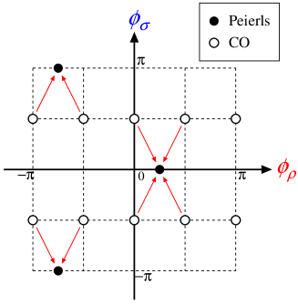
Figure 5: (Color online) Positions of the locked phase fields $\phi_{\rho}$ and $\phi_{\sigma}$ in the limits of the Peierls and CO states. The arrow indicates the schematic variation of the locking potential with increasing $u_{t}$.

For the case of large $V$, the coupling constant of the commensurability energy $g_{1/4}$ changes its sign ($g_{1/4}<0$), and favors the locking position $\phi_{\rho}=0$(mod $\pi$), which is nothing but the CO state with a twofold periodicity; i.e., $\langle n_{j}\rangle=(\,\bigcirc\,\circ\,\bigcirc\,\circ\,\cdots\,)$. In this case, the region for the lattice distortion in divided by two kinds of characteristic values $u_{t}^{\rho}$ and $u_{t}^{\sigma}$, which are given by

$$u_{t}^{\rho}\equiv\sqrt{64|g_{1/4}|g_{\sigma}},\quad u_{t}^{\sigma}\equiv 4g_{\sigma}.$$ (27)

For small $u_{t}(<u_{t}^{\rho},u_{t}^{\sigma})$, the phases $\phi_{\rho}$ and $\phi_{\sigma}$ are locked at intermediate values, while the phase $\phi_{\nu}$ takes $(\phi_{\rho},\phi_{\sigma})=(\pi/4,0)$, $(-3\pi/4,\pm\pi)$, $\ldots.$ for large $u_{t}(>u_{t}^{\rho},u_{t}^{\sigma})$. For the intermediate value of $u_{t}$, there are two possibilities: (i) $u_{t}^{\rho}\leq u_{t}^{\sigma}$ and (ii) $u_{t}^{\sigma}<u_{t}^{\rho}$. In the present paper, we focus on the former case, $u_{t}^{\rho}\leq u_{t}^{\sigma}$ (which is satisfied for $g_{1/4}<0$ and $|g_{1/4}|<g_{\sigma}/4$), since within the mean-field calculation, Omori2007 only the former case is realized and there would be some subtleties in the case of $|g_{1/4}|>g_{\sigma}/4$.

For case (i), the locking positions for the phase variables $\phi_{\rho}$ and $\phi_{\sigma}$ are analytically determined as

$$\phi_{\rho}^{\mathrm{opt}}=\left\{\begin{array}[]{ll}\displaystyle\frac{1}{2}\sin^{-1}\left(\frac{u^{2}_{t}}{u^{\rho 2}_{t}}\right)&\mbox{for }0<u_{t}<u_{t}^{\rho}\\ \\ \displaystyle\frac{\pi}{4}&\mbox{for }u_{t}^{\rho}<u_{t},\end{array}\right.$$ (28)

and

$$\phi_{\sigma}^{\mathrm{opt}}=\left\{\begin{array}[]{ll}\displaystyle\cos^{-1}\left[\frac{u_{t}}{u_{t}^{\sigma}}\sqrt{\frac{1}{2}\left(1+\frac{u_{t}^{2}}{u^{\rho 2}_{t}}\right)}\right]&\mbox{for }0<u_{t}<u_{t}^{\rho}\\ \\ \displaystyle\cos^{-1}\left(\frac{u_{t}}{u_{t}^{\sigma}}\right)&\mbox{for }u_{t}^{\rho}<u_{t}<u_{t}^{\sigma}\\ \\ 0&\mbox{for }u_{t}^{\sigma}<u_{t}.\end{array}\right.$$ (29)

The schematic variations of $\phi_{\rho}^{\mathrm{opt}}$ and $\phi_{\sigma}^{\mathrm{opt}}$ as a function of $u_{t}$ are shown in Fig. 5.

Now, we examine the energy as a function of $u_{t}$. By inserting Eqs. (28) and (29) into Eq. (21), the energy with fixed $u_{t}$ is given by $E_{0}(u_{t})\equiv V_{0}(u_{t},\phi_{\rho}^{\mathrm{opt}},\phi_{\sigma}^{\mathrm{opt}})/(2\pi^{2}a^{2})$, where

$$E_{0}(u_{t})=\left\{\begin{array}[]{lll}\displaystyle\frac{1}{2\pi^{2}a^{2}}\left[-|g_{1/4}|-g_{\sigma}+\left(\frac{K_{\mathrm{ph}}}{2}-\frac{1}{16g_{\sigma}}\right)u_{t}^{2}-\frac{u^{4}_{t}}{2^{11}|g_{1/4}|g_{\sigma}^{2}}\right]&&\mbox{for }0<u_{t}<u_{t}^{\rho}\\ \\ \displaystyle\frac{1}{2\pi^{2}a^{2}}\left[+|g_{1/4}|-g_{\sigma}+\left(\frac{K_{\mathrm{ph}}}{2}-\frac{1}{8g_{\sigma}}\right)u_{t}^{2}\right]&&\mbox{for }u_{t}^{\rho}<u_{t}<u_{t}^{\sigma}\\ \\ \displaystyle\frac{1}{2\pi^{2}a^{2}}\left[+|g_{1/4}|+g_{\sigma}-u_{t}+\frac{K_{\mathrm{ph}}}{2}u_{t}^{2}\right]&&\mbox{for }u_{t}^{\sigma}<u_{t}.\end{array}\right.$$ (35)

Typical $u_{t}$ dependencies of $E_{0}(u_{t})$ are shown in Fig. 6. For $u_{t}>u_{t}^{\rho}$, the energy $E_{0}(u_{t})$ takes a same form given in Fig. 4. It is noted that, in the present case, the energy around $u_{t}=0$ can become a local minimum; i.e., the undistorted state is realized as a metastable state. The actual ground state is determined in order to minimize the energy $E_{0}(u_{t})$ with respect to $u_{t}$. From Eq. (35), we find that the Peierls state with finite $u_{t}$ is obtained in the case of

$$g_{\sigma}+|g_{1/4}|<\frac{1}{4K_{\mathrm{ph}}}.$$ (36)

The amplitude of the lattice distortion is given by

$$u_{t}^{0}=\frac{1}{K_{\mathrm{ph}}}.$$ (37)

In addition, the condition for the Peierls state with the metastable CO state ($u_{t}=0$) is given by

$$g_{\sigma}+|g_{1/4}|<\frac{1}{4K_{\mathrm{ph}}}<2g_{\sigma}.$$ (38)

By further increasing $K_{\mathrm{ph}}\{>1/[4(g_{\sigma}+|g_{1/4}|)]\}$, we find that the energy at $u_{t}=0$ becomes lower than that of finite $u_{t}$; i.e., the first-order phase transition from the Peierls state into the CO state occurs when $1/(4K_{\mathrm{ph}})=g_{\sigma}+|g_{1/4}|$.

Figure 6: The energy $E_{0}(u_{t})$ as a function of $u_{t}$, where $u_{t}^{\sigma}=4g_{\sigma}$, and we have set $g_{1/4}/g_{\sigma}=-1/4$, The elastic constant is fixed as $g_{\sigma}K_{\mathrm{ph}}=1/3$, $1/4$, $1/5$, and $1/8$, from top to bottom. The transition point is $g_{\sigma}K_{\mathrm{ph}}=1/5$.

We note that the potential barriers from the Peierls state, $\Delta E_{\mathrm{P}}\equiv E_{0}(u_{t}^{*})-E_{0}(u_{t}^{0})$, and that from the CO state, $\Delta E_{\mathrm{CO}}\equiv E_{0}(u_{t}^{*})-E_{0}(0)$, are respectively given by

$$\Delta E_{\mathrm{P}} = \frac{1}{2\pi^{2}a^{2}}\Biggl{[}-2|g_{1/4}|-2g_{\sigma}+\frac{1}{2K_{\mathrm{ph}}}$$ (39a)

$${}+2^{9}|g_{1/4}|g_{\sigma}^{2}\left(\frac{K_{\mathrm{ph}}}{2}-\frac{1}{16g_{\sigma}}\right)^{2}\Biggr{]},$$

$$\Delta E_{\mathrm{CO}} = \frac{1}{2\pi^{2}a^{2}}2^{9}|g_{1/4}|g_{\sigma}^{2}\left(\frac{K_{\mathrm{ph}}}{2}-\frac{1}{16g_{\sigma}}\right)^{2},\qquad$$ (39b)

where $u_{t}^{*}\equiv 2^{5}|g_{1/4}|^{1/2}g_{\sigma}\sqrt{K_{\mathrm{ph}}/2-1/(16g_{\sigma})}$ is the point at which the energy takes a local maximum.

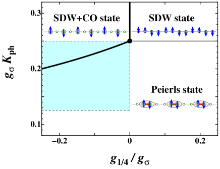
Figure 7: (color online). Ground-state phase diagram on the plane of $g_{1/4}/g_{\sigma}$ and $g_{\sigma}K_{\mathrm{ph}}$. In the shaded region, there appears a metastable state.

Based on the calculation of the ground state energy, we obtain the phase diagram on the plane of $g_{1/4}$ and $K_{\rm ph}$ shown in Fig. 7. For $g_{1/4}>0$ in which the CO state is absent, the pure SDW state is obtained for large $K_{\rm ph}$ and the Peierls state is obtained for small $K_{\rm ph}$. When $g_{1/4}<0$, the Peierls state is obtained for $4K_{\rm ph}<1/(g_{\sigma}+|g_{1/4}|)$ (region I) and the CO state coexisting with the SDW state is obtained for $4K_{\rm ph}>1/(g_{\sigma}+|g_{1/4}|)$ (region II). The metastable state at $u_{t}=0$ is obtained for $K_{\rm ph}>1/(8g_{\sigma})$ in region I, while the metastable state at $u_{t}\neq 0$ is obtained for $K_{\mathrm{ph}}<1/(4g_{\sigma})$ in region II. By taking into account the relations $g_{1/4}\propto U^{2}(U-4V)$ and $g_{\sigma}\propto U$, Tsuchiizu2001 we can obtain the ground-state phase diagram on the plane of $V$ and the elastic constant, which reproduces that of the mean-field theory. Omori2007 In section V, we examine the excited state in region I where the metastable state exists at $u_{t}=0$, as shown in Fig. 6.

V Excitations by Soliton Formations

In this section, we examine the excitations due to the soliton formations. First, we derive the equations for spatially dependent phases, which describe the variation from those of the Peierls ground state and the metastable state around $u_{t}=0$. As shown in section IV, the phase variables are uniform in space in the ground state. For simplicity, we do not consider the effect of the quantum fluctuations induced by $\theta_{\rho}$ and $\theta_{\sigma}$. Since such effects give rise to a reduction in the amplitude of the potential $V(u_{t},\phi_{\rho},\phi_{\sigma})$, it may be qualitatively understood by introducing the effective coupling constants given by $g_{1/4}^{\mathrm{eff}}=g_{1/4}\exp[-8\langle\phi_{\rho}^{2}\rangle]$, $g_{\sigma}^{\mathrm{eff}}=g_{\sigma}\exp[-2\langle\phi_{\sigma}^{2}\rangle]$, and $u_{t}^{\mathrm{eff}}=u_{\mathrm{eff}}\exp[-\frac{1}{2}(\langle\phi_{\rho}^{2}\rangle+\langle\phi_{\sigma}^{2}\rangle)]$, which can be estimated using the renormalization group treatment. Sugiura2003

We examine the classical Hamiltonian given by $H_{\mathrm{cl}}=\int dx\,\mathcal{H}_{\mathrm{cl}}$, where

$$\mathcal{H}_{\mathrm{cl}} = \frac{v_{\rho}}{4\pi K_{\rho}}\left(\frac{d\phi_{\rho}(x)}{dx}\right)^{2}+\frac{v_{\sigma}}{4\pi K_{\sigma}}\left(\frac{d\phi_{\sigma}(x)}{dx}\right)^{2}$$ (40)

$${}+\frac{1}{2\pi^{2}a^{2}}V\biglb(u_{t}(x),\phi_{\rho}(x),\phi_{\sigma}(x)\bigrb).$$

Minimizing Eq. (40) with respect to $u_{t}(x)$, $\phi_{\rho}(x)$, and $\phi_{\sigma}(x)$,Hara1983 we obtain the following equations:

$$u_{t}(x) = \frac{1}{K_{\mathrm{ph}}}\cos\left(\phi_{\rho}(x)-\frac{\pi}{4}\right)\cos\phi_{\sigma}(x),$$ (41a)

$$0 = \frac{\pi v_{\rho}a^{2}}{K_{\rho}}\frac{\partial^{2}\phi_{\rho}(x)}{\partial x^{2}}+4g_{1/4}\,\sin 4\phi_{\rho}(x)$$ (41b)

$${}-u_{t}(x)\sin\left(\phi_{\rho}(x)-\frac{\pi}{4}\right)\cos\phi_{\sigma}(x),$$

$$0 = \frac{\pi v_{\sigma}a^{2}}{K_{\sigma}}\frac{\partial^{2}\phi_{\sigma}(x)}{\partial x^{2}}+2g_{\sigma}\,\sin 2\phi_{\sigma}(x)$$ (41c)

$${}-u_{t}(x)\sin\left(\phi_{\rho}(x)-\frac{\pi}{4}\right)\sin\phi_{\sigma}(x),\qquad$$

which are self-consistently determined. Note that substituting Eq. (41a) into Eqs. (41b) and (41c), we obtain the equations for the phase variables $\phi_{\rho}(x)$ and $\phi_{\sigma}(x)$.

In the conventional picture of the soliton excitations from the Peierls ground state, Takayama1980 the charge and/or spin solitons are accompanied with the soliton of lattice distortion which connects the two minima of the potential. Due to this effect, the midgap state appears in the presence of the lattice distortion. In the present case, however, we have another excitation due to the lattice relaxation. As seen in Sec. IV, such an undistorted state ($u_{t}=0$) can be locally stabilized due to the competition between the Peierls state and the CO state. In this section, first we verify that such a metastable state can be stabilized within the reasonable choice of parameters. Next, we also consider the purely electronic excitations by considering the antiadiabatic limit where the lattice distortion is assumed to be uniform, and we estimate the magnitude of the excitation gap. These states are calculated to comprehend the state relevant to reflectivity measurements in the Peierls phase and in the photoinduced phase in (EDO-TTF)₂PF₆.

V.1 Lattice relaxations: The appearance of the charge-ordered domain in the Peierls state

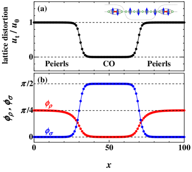
Figure 8: (Color online) (a) The lattice distortion for the coexisting CO and Peierls states (the schematic view is also shown) and (b) the corresponding soliton-antisoliton formation in the phase variables $\phi_{\rho}$ and $\phi_{\sigma}$. We have set $g_{1/4}/g_{\sigma}=-1/4$, $K_{\mathrm{ph}}=1/(5g_{\sigma})$, $K_{\rho}=0.1$, $K_{\sigma}=1$, and $v_{\rho}=v_{\sigma}=\sqrt{2}t$ with $g_{\sigma}=2t$.

We consider the case wherein both the Peierls state and the CO state become locally stable. Even for the case in which the true ground state is given by the Peierls state, it is actually expected that the Peierls state coexists with the metastable CO state without lattice distortion, in the photoexcited phase of (EDO-TTF)₂PF₆.

Figure 8 shows the coexisting state between the Peierls state and the SDW+CO state, created by the soliton-antisoliton formation connecting the different two states, which is obtained by solving Eq. (41). The parameters are set as $g_{1/4}/g_{\sigma}=-0.25$ and $g_{\sigma}K_{\mathrm{ph}}=0.2$, which correspond to the values on the boundary (see Fig. 7). The parameters for the kinetic part are chosen as $K_{\rho}=0.1$, $K_{\sigma}=1$, and $v_{\rho}=v_{\sigma}=\sqrt{2}t$. There exists a domain of the metastable CO state with $(u_{t},\phi_{\rho},\phi_{\sigma})=(0,0,\pi/2)$ in the Peierls state with $(u_{t},\phi_{\rho},\phi_{\sigma})=(u_{t}^{0},\pi/4,0)$. Note that the boundary between the Peierls and the CO states is created by the formation of solitons for charge, spin, and lattice distortion. Since such a coexisting state is expected not only for the Peierls phase at finite temperature but also for the state after the photoinduced phase transition in (EDO-TTF)₂PF₆, Chollet2005 it can be expected that such a domain stays as long as the thermal fluctuations cannot go over the potential barrier given by Eq. (39a).

V.2 Purely electronic excitations: the antiadiabatic limit

Now, we examine the excited states induced only by electronic excitations; i.e., spin and charge soliton-antisoliton excitations, while we assume that the lattice distortion remains uniform in space. This situation could be related to the electronic excitations due to the probe light in reflectivity measurements. Such a soliton excitation is also expected to play crucial roles in the photoinduced phase transition in (EDO-TTF)₂PF₆ due to the ultrafast photoresponse within the order of pico seconds. In general,Yonemitsu2006 the lattice should locally relax under friction to the minimum of the adiabatic potential, when photons are absorbed by electrons at a site.

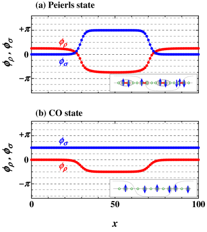
Figure 9: (Color online) Soliton-antisoliton excitation of the charge and spin phase variables, with fixed several values of (a) $u_{t}=u_{t}^{0}$ (corresponding to the Peierls state) and (b) $u_{t}=0$ (corresponding to the CO state). The soliton and/or antisoliton of $\phi_{\rho}$ and $\phi_{\sigma}$ connects two neighboring minima of $V(u_{t},\phi_{\rho},\phi_{\sigma})$ (see Fig. 5). The low-energy excitation in the Peierls state is a single-electron excitation, while that in the CO state is a domain excitation. The schematic views of the excitations for the respective cases are also shown. We have set $g_{1/4}/g_{\sigma}=-1/4$ and $K_{\mathrm{ph}}=3/(16g_{\sigma})$ with $g_{\sigma}=2t$, $K_{\rho}=0.1$, and $K_{\sigma}=1$.

To this end, we calculate Eqs. (41b) and (41c) with the fixed uniform $u_{t}$, for the Peierls state ($u_{t}=u_{t}^{0}$) and the CO state ($u_{t}=0$). In the Peierls state corresponding to finite $u_{t}$ $(=u_{t}^{0})$, the soliton-antisoliton excitation is characterized as

$$(\phi_{\rho},\phi_{\sigma})=\left(\frac{\pi}{4},0\right)\to\left(-\frac{3\pi}{4},\pi\right)\to\left(\frac{\pi}{4},0\right).$$ (42)

The explicit profile is shown in Fig. 9(a). Thus, the soliton-antisoliton excitation in the Peierls state carries the topological charge $Q=\pm 1$ and the spin $S_{z}=\pm 1/2$, Tsuchiizu2004 which is nothing but a single-electron excitation. The simple picture is the following: A particle at the position of the soliton moves away from the place of the antisoliton by breaking the spin-singlet state. Then, one finds an emergence of a local spin with a hole around the soliton kink and that of a local spin with an extra electron around the antisoliton kink. On the other hand, the soliton in the CO state is given by [Fig. 9(b)],

$$(\phi_{\rho},\phi_{\sigma})=\left(0,\frac{\pi}{2}\right)\rightarrow\left(-\frac{\pi}{2},\frac{\pi}{2}\right)\rightarrow\left(0,\frac{\pi}{2}\right),$$ (43)

which carries the topological charge $Q=\pm 1/2$ and $S_{z}=0$. A noticeable feature is seen from the fact that only the charge excitation occurs. This is a typical domain excitation in the CO state. The charge increases at the kink of the soliton and the extra hole appears at the kink of the antisoliton.

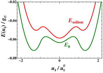
Figure 10: (Color online) Ground-state ($E_{0}$) and soliton-antisoliton formation ($E_{s}$) energies as a function of $u_{t}$, where we have set $g_{1/4}/g_{\sigma}=-1/4$ and $K_{\mathrm{ph}}=3/(16g_{\sigma})$ with $g_{\sigma}=2t$, $K_{\rho}=0.1$, and $K_{\sigma}=1$.

As shown in Fig. 5, the locking location of the phase variables $\phi_{\rho}$ and $\phi_{\sigma}$ changes depending on the strength of the lattice distortion $u_{t}$. Even though the state with the intermediate values of $0<u_{t}<u_{t}^{0}$ is not stable, we can consider the purely electronic soliton excitations in such a virtual state and discuss the “$u_{t}$ dependence” of the soliton excitation energy. The $u_{t}$ dependence of the ground-state energy and the soliton-antisoliton energy is shown in Fig. 10. Here, we assumed that the soliton and antisoliton do not form a bound state (breather) and estimated the soliton-antisoliton formation energy by doubling the soliton energy in Fig. 9. From Fig. 10, it is found that the soliton formation energy in the CO state costs less energy compared with that in the Peierls state. This is due to the fact that only the charge degree of freedom participates in for the CO state. From this excitation energy analysis, it can be found that both the Peierls state ($u_{t}=u_{t}^{0}$) and the CO state ($u_{t}=0$) have finite energy gaps to the excited states; i.e., both states are insulators. However, in the CO state, the system could have a semiconducting feature since the gap can become very small. The magnitude of this energy gap depends on the choice of parameters, but it is discussed by comparing the mean-field results in Sec. VI.

There are many choices of creating solitons in Fig. 9; however, the present estimation has been done for the soliton, which has the minimum energy for large $u_{t}$ limit and is adiabatically connected to the small $u_{t}$ case. From this excitation energy analysis, it can be found that the one-particle excitations in the Peierls state could be related to the domain excitations in the CO state. Such a connectivity would be relevant to the photoinduced phase transition mechanism, but this needs further investigation.

VI Summary and Discussions

We have examined the exotic Peierls state observed in (EDO-TTF)₂PF₆ and analyzed the excitation from the Peierls ground state and also the excitation from the metastable CO state. The metastable CO state around the CO state has been found by considering the modulation of the elastic constants $\delta K_{P}$ and $\delta K_{H}$ and by considering the moderate strength of the nearest neighbor repulsive interaction. The metastable state, which coexists with the spin-density wave, exhibits soliton excitations, having an energy much smaller than that of the Peierls state. The energy of the ground state and the excited state, which are obtained as a function of $u_{t}$, exhibits a common feature with the adiabatic potential in the electron-phonon coupled system in one dimension. Koshino1998 Considering the correspondence between such a situation to the case of EDO-TTF, the present metastable state could be relevant to the state of the photoinduced phase.

Here, we discuss the experimental findings on the reflectivity in the photoinduced phase of (EDO-TTF)₂PF₆ based on the present analysis. From the photoconductivity measurement, the photoinduced phase exhibits a metallic behavior, although it is not the same as that of high-temperature metallic state, as shown by the reflectivity data.Onda2005 In the present analysis, we obtained the metastable state without lattice distortion, which is not the normal state. Actually, in such a state, the translational invariance is broken due to the presence of the CO state, which gives a small soliton excitation gap. Here, we estimate the magnitude of the soliton gaps. From the mean-field approach, Suzumura1997 the commensurability potential is estimated as $C_{0}\cos 4\phi_{\rho}$, where the amplitude is given by $C_{0}\approx-0.03t$ for $(U/t,V/t)=(4,2)$. On the other hand, the amplitude of the $\cos 2\phi_{\sigma}$ potential Tomio2000JPSJ is about $0.15t\sim 0.3t$, which are estimated from $(V/t,V_{2}/t)\approx(1.4,\,1.05)\sim(2,\,0)$. Thus, we find $g_{1/4}/g_{\sigma}\approx-0.1\sim-0.2$ and our choice of the parameter $g_{1/4}/g_{\sigma}=-1/4$ in Fig. 10 is not far from the mean-field results. Actually, we obtain $g_{\sigma}/(2\pi^{2}a^{2})=-4g_{1/4}/(2\pi^{2}a^{2})=0.12t$ from the mean-field result, $C_{0}(V=2t)\approx-0.03t$. Here, we note the soliton gap at $u_{t}=0$, which is of the order of $\delta E(0)=[E_{\mathrm{soliton}}(0)-E_{0}(0)]\approx 0.01t$, and then $\delta E(0)\approx 3$ meV. On the other hand, the soliton gap from the Peierls ground state is given by $\delta E(u_{t}^{\mathrm{opt}})=[E_{\mathrm{soliton}}(u_{t}^{\mathrm{opt}})-E_{0}(u_{t}^{\mathrm{opt}})]\approx 0.045t\approx 14$ meV, which is much larger than that of the metastable state.

Finally, we comment on the quantum fluctuation on the lattice distortion, which is not treated in the present calculation. Such an effect appears when the term $\sum_{j}P_{j}^{2}/2M$ is taken into account for Eq. (3c) with $[u_{j},P_{j^{\prime}}]=\delta_{j,j^{\prime}}$. The present calculation corresponds to the limit of a large mass $M$. If we naively consider a renormalization by a Debye$-$Waller factor, Ziman the effective coupling constant $g_{\mathrm{ph}}$ is reduced due to the quantum fluctuation. Thus, this fluctuation makes the normalized constant $K_{\mathrm{ph}}$ large and the region for CO in Fig. 7 is extended. For the limit of the light mass, which corresponds to the antiadiabatic case, the averaged lattice distortion vanishes but the crossover from the spin-density-wave state to the spin singlet is expected with an increase in the electron-phonon coupling constant $g_{\rm ph}(>\sqrt{K_{\rm ph}U})$. Yonemitsu1996PRB ; Tsuchiizu2005 Thus, the metastable state, which coexists with the CO and spin-density-wave states due to the electronic correlations, is expected to give rise to the conduction by forming the solitary charge excitation if the quantum fluctuations of both the electron and the phonon remain moderately small.

- (1) M. Chollet, L. Guerin, N. Uchida, S. Fukaya, H. Shimoda, T. Ishikawa, K. Matsuda, T. Hasegawa, A. Ota, H. Yamochi, G. Saito, R. Tazaki, S. Adachi, and S. Koshihara, Science 307, 86 (2005).
- (2) K. Onda, T. Ishikawa, M. Chollet, X. Shao, H. Yamochi, G. Saito, and S. Koshihara, J. Phys: Conf. Ser. 21, 216 (2005).
- (3) S. Koshihara and S. Adachi, J. Phys. Soc. Jpn. 75, 011005 (2006).
- (4) A. Ota, H. Yamochi, and G. Saito, J. Mater. Chem. 12, 2600 (2002); A. Ota, H. Yamochi, and G. Saito, Synth. Met. 133-134, 463 (2003).
- (5) O. Drozdova, K. Yakushi, A. Ota, H. Yamochi, and G. Saito, Synth. Met. 133-134, 277 (2003); O. Drozdova, K. Yakushi, K. Yamamoto, A. Ota, H. Yamochi, G. Saito, H. Tashiro, and D. B. Tanner, Phys. Rev. B 70, 075107 (2004).
- (6) Y. Tokura, J. Phys. Soc. Jpn. 75, 011001 (2006).
- (7) K. C. Ung, S. Mazumdar, and D. Toussaint, Phys. Rev. Lett. 73, 2603 (1994).
- (8) R. T. Clay, S. Mazumdar, and D. K. Campbell, Phys. Rev. B 67, 115121 (2003).
- (9) M. Kuwabara, H. Seo, and M. Ogata, J. Phys. Soc. Jpn. 72, 225 (2003).
- (10) H. Seo, Y. Motome, and T. Kato, J. Phys. Soc. Jpn. 76, 013707 (2007).
- (11) Y. Omori, M. Tsuchiizu, and Y. Suzumura, J. Phys. Soc. Jpn. 76, 114709 (2007).
- (12) T. Mori, A. Kobayashi, Y. Sasaki, H. Kobayashi, G. Saito, and H. Inokuchi, Bull. Chem. Soc. Jpn. 57, 627 (1984); T. Mori, Ph.D. thesis, University of Tokyo, 1985.
- (13) M. Sugiura, and Y. Suzumura, J. Phys. Soc. Jpn. 72, 1458 (2003); M. Sugiura, M. Tsuchiizu, and Y. Suzumura, ibid. 74, 983 (2005).
- (14) For a review, see T. Giamarchi, Quantum Physics in One Dimension (Oxford University Press, New York, 2004).
- (15) H. Fukuyama and H. Takayama, in Electronic Properties of Inorganic Quasi-One-Dimensional Compounds, ed. P. Monceau (Reidel, Dordrecht, 1985), p. 41.
- (16) M. Tsuchiizu, H. Yoshioka, and Y. Suzumura, J. Phys. Soc. Jpn. 70, 1460 (2001).
- (17) J. Hara and H. Fukuyama, J. Phys. Soc. Jpn. 52, 2128 (1983).
- (18) H. Takayama, Y. R. Lin-Liu, and K. Maki, Phys. Rev. B 21, 2388 (1980).
- (19) K. Yonemitsu and K. Nasu, J. Phys. Soc. Jpn. 75, 011008 (2006).
- (20) M. Tsuchiizu and A. Furusaki, Phys. Rev. B 69, 035103 (2004).
- (21) K. Koshino and T. Ogawa, J. Phys. Soc. Jpn. 67, 2174 (1998).
- (22) Y. Suzumura, J. Phys. Soc. Jpn. 66, 3244 (1997).
- (23) Y. Tomio and Y. Suzumura, J. Phys. Soc. Jpn. 69, 796 (2000).
- (24) J. M. Ziman, Principles of the Theory of Solids (Cambridge University Press, Cambridge, 1965), p. 60.
- (25) K. Yonemitsu and M. Imada, Phys. Rev. B 54, 2410 (1996).
- (26) M. Tsuchiizu, M. Sugiura, and Y. Suzumura, Physica B (Amsterdam) 358, 42 (2005).