Adaptive Independent Metropolis-Hastings by Fast Estimation of Mixtures of Normals

Abstract

Adaptive Metropolis-Hastings samplers use information obtained from previous draws to tune the proposal distribution automatically and repeatedly. Adaptation needs to be done carefully to ensure convergence to the correct target distribution because the resulting chain is not Markovian. We construct an adaptive independent Metropolis-Hastings sampler that uses a mixture of normals as a proposal distribution. To take full advantage of the potential of adaptive sampling our algorithm updates the mixture of normals frequently, starting early in the chain. The algorithm is built for speed and reliability and its sampling performance is evaluated with real and simulated examples. Our article outlines conditions for adaptive sampling to hold and gives a readily accessible proof that under these conditions the sampling scheme generates iterates that converge to the target distribution.

Keywords: Clustering; Gibbs sampling; Markov chain Monte Carlo; Semiparametric regression models; State space models.

1 Introduction

Bayesian methods using Markov chain Monte Carlo (MCMC) simulation have greatly influenced statistical and econometric practice over the past fifteen years because of their ability to estimate complex models and produce finite sample inference. A key component in implementing MCMC simulation is the Metropolis-Hastings (MH) method (Metropolis et al. 1953; Hastings 1970), which requires the specification of one or more proposal distributions. The speed at which the chain converges to the posterior distribution and its ability to move efficiently across the state space depend crucially on whether the proposal distribution(s) provide good approximations to the target distributions, either locally or globally. Given the key role played by proposal distributions, it is natural to use experience from preliminary runs to tune or adapt the proposal to the target. We define strict adaptation as adaptation that is subject to theoretical rules which ensure that the iterates converge to realizations from the correct target (posterior) distribution. All other adaptation of the MH kernel will be called preliminary adaptation, whose purpose is either to obtain an adequate proposal density before switching to non-adaptive MCMC sampling, or as the starting point for strict adaptive sampling.

Despite the different theoretical requirements of preliminary and strict adaptation, a great deal of care is needed in constructing both types of adaptive sampling schemes because the ultimate goal is to obtain reliable estimates of functionals of the target distribution as quickly as possible.

The literature on adaptive MCMC methods follows two main strands. Adaptation by regeneration stems from the work of Gilks et al. (1998). Our article focuses exclusively on diminishing adaptation schemes. Important theoretical advances in diminishing adaptation were made by Holden (1998), Haario et al. (2001), Andrieu and Robert (2001), Andrieu and Moulines (2006), Andrieu et al. (2005), Atchadé and Rosenthal (2005), Nott and Kohn (2005) and Roberts and Rosenthal (2007). The proofs of convergence for strict adaptive sampling are more complex than for the non adaptive case as the iterates are not Markovian because the MH kernel can depend on the entire history of the draws. Although more theoretical work on adaptive sampling can be expected, the existing body of results provides sufficient justification and guidelines to build adaptive MH samplers for challenging problems.

Research is now needed on how to design efficient and reliable adaptive samplers for broad classes of problems. This more applied literature mostly focuses on random walk Metropolis, see for example Roberts and Rosenthal (2006). Partial exceptions are Gåsemyr (2003) who uses normal proposals for an independent Metropolis-Hastings, but limits the tuning of the parameters to the burn-in period, and Hastie (2005), who mixes random walk and independent MH in reversible jump problems, in what we call two step adaptation in section 2. Independent MH schemes are implemented by Nott and Kohn (2005) to sample discrete state spaces in variable selection problems (e.g. to learn if a variable is in or out), and by Giordani and Kohn (2008) to learn about interventions, such as breaks or outliers, in dynamic mixture models.

Our paper contributes to the development of both preliminary and strict algorithms for adaptive independent MH sampling in continuous state spaces. Increased sampling efficiency is obviously one important goal, particularly in cases where current best practice (typically some version of random walk Metropolis or Gibbs sampling) is less than satisfactory. But equally important achievements of adaptive schemes may be to expand the set of problems that can be handled efficiently by general purpose samplers and to reduce coding effort. In particular, adaptive schemes can reduce dependence on the use of conjugate priors. Such priors make it easier to implement MCMC schemes, but are less necessary when using adaptive sampling.

Our adaptive sampling approach is built on four main ideas. The first is to combine preliminary and strict adaptation into one estimation procedure. The second is to estimate mixtures of Gaussians from the history of the draws and use them as proposal distributions for independent MH in both parts of the adaptation. The third is to perform this estimation frequently, particularly during the preliminary adaptation stage, a strategy we call intensive adaptation. The fourth is to ensure that the theoretical conditions for the correct ergodic behavior of the sampler are respected during strict adaptation. To apply these ideas successfully, estimation of the mixture parameters needs to be fast, reliable, and robust. We achieve a good balance of these goals by carefully selecting and tailoring to our needs algorithms developed in the clustering literature.

We study the performance of our adaptive sampler in three examples in which commonly used Gibbs schemes can be very inefficient and compare it with an adaptive random walk Metropolis sampler proposed by Roberts and Rosenthal (2006) that builds on the work .

Our paper also provides conditions and outlines a proof that our strict adaptive sampling scheme converges to the correct target distribution and gives convergence rates.

2 Two-step adaptation and intensive adaptation

A necessary condition for a successful adaptive independent Metropolis-Hastings (AIMH) sampler is that, given a sizable sample drawn from the target $\pi(z)$, the suggested algorithm can build a proposal $q(z)$ which is sufficiently close to the target for IMH to perform adequately. A two-step adaptive strategy is also feasible whenever the answer is positive. We loosely define two-step adaptation as a sampling scheme in which a rather thorough exploration of the target density is carried out in the first part of the chain by a sampler other than IMH (such as random walk Metropolis) before switching to a more efficient IMH sampler with proposal density tuned on the first-stage draws. An early version of such a two-step procedure is proposed by Gelman and Rubin (1992). Hastie (2005) provides an interesting application to reversible jump problems.

Two-step adaptation is relatively simple and safe and in some cases is capable of achieving sizable efficiency gains. However, it has the following limitations. First, if the first stage sampler fails to adequately explore a region of the state space, the proposal built for the second stage will also inadequately cover that region. To reduce this risk we may need a very large number of iterations in the first phase, which may be particularly time consuming if the first stage sampler is inefficient. Second, there may be no saving of coding effort if the first stage sampler generates from several conditional distributions, as in Gibbs or Metropolis-within-Gibbs, in order to be efficient.

We loosely define intensive adaptation as an AIMH scheme in which the proposal distribution is updated frequently, particularly in the early part of the chain. Building a sequence of increasingly good proposal densities in intensive adaptation is more demanding than building a proposal density once based on thousands of draws. The question is whether we can adequately explore the target distributions given an initial proposal $g_{0}(z)$ but no draws. The answer inevitably depends on the initial proposal $g_{0}(z)$, on the target $\pi(z)$, and on the details of the sampling scheme. However, it is possible to outline some general dangers and opportunities offered by intensive adaptation.

Among the advantages, if the proposal distribution is sufficiently flexible, frequent tuning of its parameters and continuing adaptation for the entire length of the chain reduces the risk of a long run of rejections and increases the chances of good performance when the initial proposal approximates the target poorly.

Estimating proposal densities based on a small number of draws presents some dangers that the designer of an AIMH scheme should try to minimize. For example, suppose that we predetermine the iteration, say $j$, at which the proposal is first updated. If the first $j$ draws have all been rejected, then a proposal distribution based entirely on these draws is degenerate and makes the chain reducible. If too few draws have been accepted, the proposal may be very poor. We employ the following strategy to prevent these outcomes. First, we initially update the proposal at a predetermined number of accepted draws. Second, after fitting a mixture of normal distributions to past draws, we fatten and stretch its tails by creating a mixture of mixtures as described in section 3. Third, we let the proposal be a mixture where one component is the initial proposal $g_{0}(z)$, which should of course have long tails. This is similar to the defensive mixtures approach studied by Hesterberg (1998) for importance sampling. The same provisions reduce the risk of adapting too quickly to a local mode.

3 Some theory for adaptive sampling

A diminishing adaptation MH sampler performs the accept/reject step like a standard MH, but updates the proposal distribution using the history of the draws. This updating is ‘diminishing’ in the sense that the proposal distribution settles down asymptotically (in the number of iterations).

This section outlines the theoretical framework for strict adaptive independent Metropolis-Hastings sampling as used in our article that gives some support for our practice. The appendix outlines proofs of the theoretical results, which extend similar results in Nott and Kohn (2005) for the case of a finite state space. Our aim is to provide simple accessible proofs that will help to popularize the adaptive methodology. All densities in this section are with respect to Lebesgue measure or counting measure, which we denote as $\mu\{\cdot\}$.

Let $\cal Z$ be a sample space and $\pi(z)$ a target density on $\cal Z$. We use the following adaptive MH scheme to construct a sequence of random variables $\{Z_{n},n\geq 2\}$ whose distribution converges to $\pi(z)$. We assume that $Z_{0}$ and $Z_{1}$ are generated independently from some initial density $q_{I}(z)$. In our examples, this is a heavy tailed version of the Laplace approximation to the posterior distribution. For $n\geq 1$, let $q_{n}(z;\lambda_{n})$ be a proposal density for generating $Z_{n+1}$, where $\lambda_{n}$ is a parameter vector that is based on $Z_{0}=z_{0},\dots,Z_{n-1}=z_{n-1}$. Thus, given $Z_{n}=z$, we generate $Z_{n+1}=z^{\prime}$ from $q_{n}$, and then with probability

$$\alpha_{n}(z,z^{\prime}) =\min\biggl{(}1,\frac{\pi(z^{\prime})}{\pi(z)}\frac{q_{n}(z;\lambda_{n})}{q_{n}(z^{\prime};\lambda_{n})}\biggr{)}$$ (1)

we take $Z_{n+1}=z^{\prime}$; otherwise we take $Z_{n+1}=z$. Our choice of $q_{n}(z;\lambda_{n})$ is

$$q_{n}(z;\lambda_{n}) =\omega_{1}g_{0}(z)+(1-\omega_{1})\bar{g}_{n}(z;{\bar{\lambda}}_{n})$$ (2)

where $0<\omega_{1}<1$ and the density $g_{0}(z)$ does not depend on $\lambda_{n}$. We usually fix $\omega_{1}$ so that $\lambda_{n}={\bar{\lambda}}_{n}$; otherwise $\lambda_{n}=({\bar{\lambda}}_{n},\omega_{1})$. The density $\bar{g}_{n}(z;{\bar{\lambda}}_{n})$ is an approximation to $\pi(z)$ whose form is discussed below, in section 5 and in appendix 1. We assume that there exists a constant $K>0$ such that for all $z\in\cal Z$

$$\frac{\pi(z)}{g_{0}(z)}\ \leq\ K,\quad\frac{\bar{g}_{n}(z;{\bar{\lambda}}_{n})}{g_{0}(z)}\ \leq\ K\ ,\quad\text{and}\quad\frac{q_{I}(z)}{g_{0}(z)}\ \leq\ K$$ (3)

and

$$\sup_{z\in\cal Z}\biggl{|}\biggl{(}\bar{g}_{n}(z;{\bar{\lambda}}_{n})-\bar{g}_{n+1}(z;{\bar{\lambda}}_{n+1})\biggr{)}/g_{0}(z)\biggr{|} =a_{n}$$ (4)

where $a_{n}=O(n^{-r})$ for some $r>0$ almost surely. If $\cal Z$ is compact then (3) holds almost automatically. If, in addition, ${\bar{\lambda}}_{n}$ is based on means and covariances of the $z$ iterates then we can show that $\mid\mid{\bar{\lambda}}_{n}-{\bar{\lambda}}_{n+1}\mid\mid=O(n^{-1})$ and equation (4) also holds. In relation to (3), we note that in the non-adaptive case, that is $q_{n}(z;\lambda_{n})=q(z)$ for all $n$, Mengersen and Tweedie (1996) show that $\pi(z)/q(z)\leq K$ for all $z$ is a necessary and sufficient condition for geometric ergodicity.

Under conditions (3) and (4), the following results are proved in Appendix 2.

Theorem 1

For all measurable subsets $A$

$$\sup_{A\subset\cal Z}\mid\Pr(Z_{n}\in A)-\pi(A)\mid \rightarrow 0\quad\text{as}\quad n\rightarrow\infty.$$ (5)

Theorem 2

Suppose that $h(z)$ is a measurable function that is square integrable with respect to the density $g_{0}$. Then, almost surely,

$$\frac{1}{n}\sum_{j=1}^{n}h(Z_{j})\rightarrow E_{\pi}(h(Z))\quad\text{as }\quad n\rightarrow\infty.$$ (6)

We now describe the form of $\bar{g}_{n}(z;{\bar{\lambda}}_{n})$ in (2). For conciseness, we shall often omit showing dependence on $\lambda$; e.g. we will write $\bar{g}_{n}(z;{\bar{\lambda}}_{n})$ as $\bar{g}_{n}(z)$. Let $g^{\star}_{n}(z)=g^{\star}_{n}(z;{\lambda}^{\star}_{n})$ be a mixture of normals obtained using k-harmonic means clustering as described in section 5 and appendix 1, and let ${\tilde{g}}^{\star}_{n}(z)$ be a second mixture of normals having the same component weights and means as $g^{\star}_{n}(z)$, but with its component variances inflated by a factor $k>1$. Let

$${\bar{g}}^{*}_{n}(z) =\omega_{2}^{\prime}{\tilde{g}}^{\star}_{n}(z)+(1-\omega_{2}^{\prime})g^{\star}_{n}(z)\ ,$$ (7)

where $\omega_{2}^{\prime}=\omega_{2}/(1-\omega_{1})$ with $\omega_{1}$ defined in (2), $\omega_{1}>0,\omega_{2}>0$, and $\omega_{1}+\omega_{2}<1$. We note that ${\bar{g}}^{*}_{n}(z)$ is also a mixture of normals, and we say that ${\bar{g}}^{*}_{n}(z)$ is obtained by ‘stretching and fattening’ the tails of $g^{\star}_{n}(z)$. This strategy for obtaining heavier tailed mixtures is used extensively in our paper.

To allow for diminishing adaptation, we introduce the sequence $\beta_{n}$, where $0\leq\beta_{n}\leq 1$, and define

$$\bar{g}_{n}(z) =(1-\beta_{n}){\bar{g}}^{*}_{n}(z)+\beta_{n}\bar{g}_{n-1}(z)$$ (8)

with $\bar{g}_{n}(z)=\bar{g}_{n}(z;{{\bar{\lambda}}}_{n})$, where ${{\bar{\lambda}}}_{n}$ is a function of ${\lambda}^{\star}_{n}$ and $\beta_{n}$. Alternatively, we can define

$${\bar{\lambda}}_{n} =(1-\beta_{n})\lambda_{n}^{\star}+\beta_{n}{\bar{\lambda}}_{n-1}$$ (9)

and $\bar{g}_{n}(z)=\bar{g}_{n}(z;{{\bar{\lambda}}}_{n})$.

If we restrict $\cal Z$ to be compact and let $\beta_{n}\rightarrow 1$ at an appropriate rate then it is straightforward to check in most cases that the dominance and diminishing adaptation conditions, (3) and (4), hold. If $\cal Z$ is unconstrained but we restrict the $\lambda_{n}^{\star}$ to lie in a bounded set then we can do rough empirical checks that (3) and (4) hold by taking $g_{0}(z)$ to be sufficiently heavy tailed. In our empirical examples we often find that we can take $\beta_{n}=0$ for all $n$ because $\lambda_{n}^{\star}$ converges to a $\lambda^{\star}$ at a sufficiently fast rate as $n$ increases. This means that if $g_{0}(z)$ is sufficiently heavy tailed then (3) and (4) hold as $n$ increases.

Section 7 and appendix F of Andrieu and Moulines (2006) give general convergence results for adaptive independent Metropolis-Hastings and Roberts and Rosenthal (2007) give an elegant proof of the convergence of adaptive sampling schemes. However, we believe that readers may find the conditions (3) and (4) and the proofs of Theorems 1 and 2 easier to understand for the methodology proposed in our article.

4 Implementation of the adaptive sampling scheme

This section outlines how our sampling scheme is implemented. We anticipate that readers will use this as a basis for their own experimentation. In the preliminary phase the density $g_{0}(z)$ in (2) is a mixture of the Laplace approximation to the posterior and a heavier tailed version of the Laplace approximation, using weights of 0.6 and 0.4. By a heavier tailed version we mean a distribution with the same mean but with a covariance matrix that is 25 times larger. If the Laplace approximation is unavailable, then we use the prior. At the end of the preliminary phase, $g_{0}(z)$ is constructed as a mixture of the last estimated mixture, which we call $g_{\text{last}}(z)$ say, and a heavier tailed version of $g_{\text{last}}(z)$. That is, the component weights and means are set to those of $g_{\text{last}}(z)$, and its component variances equal to $k=25$ times the component variances of $g_{\text{last}}(z)$.

In our empirical work we set the weights $\omega_{1}=0.05,$ and $\omega_{2}=0.15$ in (2) and (7). We also inflate the component variances of $g_{n}^{*}(z)$ by a factor of $k=16$ to obtain the corresponding variances of $\widetilde{g}_{n}^{*}(z)$. These values have been found to work well but are not optimal in any specific sense. We conjecture that the speed of convergence and efficiency of our sampler could be further improved with a more careful (and possibly adaptive) choice of these parameters. Any other value of $k$ in the range $9$-$25$ and of $\omega_{1}$ and $\omega_{2}$ in the range $0.05-0.3$ worked well for the examples given in this paper, and $\omega_{1}$ could be set to 0 in the preliminary phase without affecting the results.

In our empirical work, during the preliminary phase, when there are 2 to 4 unknown parameters as in the inflation and stochastic volatility examples, we first re-estimate the k-harmonic means mixture after 20 accepted draws in order to ensure that the estimated covariance matrices are positive definite. If our parameter space is bigger then we would increase that number appropriately. We then re-estimate the mixture after 50, 100, …, 350, 400, 500, …, 1000, 1500, …, 3000 draws and then every 1000 draws thereafter. We also recommend updating the proposal following a period of low acceptance probabilities in the MH step. Specifically, we re-estimate the mixture parameters if the average acceptance probability in the last $L$ iterations is lower than $\alpha_{L}$, where we set $\alpha_{L}=0.1$ and $L=10$. Low acceptance probabilities signal a poor fit of the proposal, and it is therefore sensible to update the proposal to give it a better chance of covering the area around the current parameter value. Since it is unclear that this does not violate any of the conditions required for the ergodicity of our adaptive sampler, we limit the updating of the proposal at endogenously chosen points to a preliminary period, after which the proposal is updated only at predetermined intervals. The end of the preliminary adaptation period could be set ex-ante, but we prefer to determine it endogenously by requiring the smallest acceptance probability in the last $M$ iterations to be higher than $\alpha_{M},$ where $M$ is set to 500 and $\alpha_{M}$ to 0.02. During the period of strict adaptation, we update the proposal every 1000 draws.

We conjecture that Theorems 1 and 2 will still hold if we update the proposal after a sequence of low acceptance probabilities so that we could also use this update strategy during the period of strict adaptation. However, we have not implemented this in our empirical analyses.

The estimation of the mixture of normals can become slow when the number of iterations is large. To avoid this problem, after $1000$ accepted draws we only add every $j$-$th$ draw to the sample used to estimate the mixture parameters, where $j$ is chosen so that the mixture is not estimated on more than $10000$ observations.

When most parameters are nearly normally distributed, fitting a mixture of normals to all the parameters is problematic in the sense that the chances of finding a local mode with all parameters normally distributed is quite high (though depending on the starting value of course). This is true of clustering algorithms and also of EM-based algorithms. To improve the performance of the sampler in these situations, we divide the parameter vector $\theta$ into two groups, $\theta_{1}$ and $\theta_{2}$, where parameters in $\theta_{1}$ are classified as approximately normal and parameters in $\theta_{2}$ are skewed. A normal is then fit to the first group and a mixture of $p$ normals to the second. For $\theta_{1}$, we can compute the mean $\mu_{\theta_{1}}$ and covariance matrix $\Sigma_{\theta_{1}}$ inexpensively from the draws. For $\theta_{2},$ we fit a mixture of normals as detailed below, estimating probabilities $\pi_{1},...,\pi_{p},$ means $\mu_{1},...,\mu_{p},$ and covariance matrices $\Sigma_{1},...,\Sigma_{p}.$ We then need to build a mixture for $\theta=\{\theta_{1},\theta_{2}\}$. The mean is straightforward: for the normal parameters, all components have the same mean. The diagonal blocks of the covariance matrices $\Omega_{i}$ corresponding to $\text{var}(\theta_{1})$ and $\text{var}(\theta_{2})$ for component $i$ are also straightforward. The off-diagonal blocks of $\Omega_{i},$ corresponding to $\text{cov}(\theta_{1},\theta_{2})$ is computed as

$$\Omega_{i}^{12}=\sum_{t=1}^{n}\pi_{i,t}^{\ast}[(\theta_{1,t}-\mu_{\theta_{1}})(\theta_{2,t}-\mu_{i})]/\sum_{t=1}^{n}\pi_{i,t}^{\ast},$$

where $\pi_{i,t}^{\ast}=\Pr(K_{t}=i|\theta_{2,t})$ is the probability of $\theta_{2,t}$ coming from the $i$-th component.

5 A clustering algorithm for fast estimation of mixtures of normals in adaptive IMH

Finite mixtures of normals are an attractive option to construct the proposal density because they can approximate any continuous density arbitrarily well and are fast to sample from and evaluate. See McLachlan and Peel (2000) for an extensive treatment of finite mixture models.

However, estimating mixtures of normals is already a difficult problem when an independent and identically distributed sample from the target is given and estimation needs to be performed only once: the likelihood goes to infinity whenever a component has zero variance (an even more concrete possibility if, as unavoidable in IMH, some observations appear more than once), and its maximization, whether by the EM algorithm or directly, is plagued by local modes. Although several authors have made substantial advances in dealing with these problems (e.g. Figuereido and Jain 2002; Ueda, Nakano, Ghahramani, and Hinton 2000; Verbeek, Vlassis, and Krose 2003), in our experience the EM algorithm does not seem to be sufficiently reliable when the sample is small and contains a non-trivial share of rejected draws. The inevitable short runs of rejections give rise to small clusters with zero covariance matrix at which the EM algorithm frequently gets stuck. Moreover, EM-based algorithm are computationally expensive and slow to converge, which makes them less attractive when the proposal is to be updated frequently.

We have therefore limited our attention to algorithms that estimate mixtures of normals quickly and without explicitly computing the covariance matrix of each component (for robustness). Within this class, the k-means is the most popular algorithm. We employ the k-harmonic means, an extension of the k-means algorithm that allows for soft membership. Degeneracies can be easily prevented, so the algorithm is remarkably robust even in the presence of a long series of rejections. The number of clusters is chosen with the BIC criterion. The increase in speed and reliability is paid for with a decreased fit to the target, as the family of k-means algorithms performs best when an optimal fit requires all components of the mixture to have the same probability and covariance matrix (see Bradly and Fayyad 1998, for a discussion). Hamerly and Elkan (2002) show that the performance of k-harmonic means deteriorates less rapidly than alternatives of similar computational cost with departures from these ideal conditions. An outline of the k-harmonic means algorithms is given in Appendix 1.

Although the k-harmonic means algorithm is less sensitive to initialization than either k-means or EM (Hamerly and Elkan 2002), in an unsupervised environment it is important to have good starting values. We have found the algorithm of Bradly and Fayyad (1998) to perform very well and at a low computational cost.

If the proposal distribution is normal then it is computationally inexpensive to update it at every iteration. It is tempting to update a mixture of normals proposal with an on-line estimation procedure such as the on-line EM algorithm proposed in Andrieu and Moulines (2006). The advantage of on-line estimation is that the parameters of the mixture are updated recursively, so the proposal itself is updated at each iteration at a very small computational cost. However, on-line estimation of the mixture parameters in AIMH has a number of serious shortcomings. The estimates are inefficient compared to batch estimators because each data point is used only once, which corresponds to requiring a batch optimization to converge in one step. The loss of efficiency is more severe in small samples, that is, in the early phases of the chain. Direct estimation of the mixture component covariance matrices often leads to numerical problems in the early phases of the chain given that rejections in MH produce degenerate clusters. Finally, a limitation of on-line estimators is related to the fact that they are a form of stochastic gradient descent (see Spall (2003) for an introduction). When the function to be maximized is multimodal (as typically the case with mixtures) on-line estimates are in general sensitive to the order of the draws, with initial draws having heavier influence than later draws in determining the mode at which estimates settle down. We have verified empirically that the quality of solutions given by several on-line algorithms deteriorates rapidly if the initial observations are not representative of the entire target distribution. This makes on-line algorithms unsuitable for use in the early, exploratory phases of the chain, though they can work well if the initial proposal distribution already provides a reasonably good approximation of the target and the acceptance rates are sufficiently high.

Since we are opting for batch estimators, it is too costly to update the proposal at each iteration. We update it at predetermined numbers of iterations, more frequently in the earlier stages of the chain. Implementation details for the empirical examples are given in section 4.

We make two further comments on Andrieu and Moulines (2006). First, they propose to keep the number of components in the mixture constant, whereas we have found it advantageous to select the number adaptively as outlined in appendix 1. Second, they outline a proposed approach to using mixtures as proposal densities, but do not report on the empirical performance of their proposal.

6 Discussion

In order to understand the strengths and limitations of our sampler, we have found it useful to consider two desirable qualities of an adaptive IMH scheme. First, given a sufficiently large sample drawn from the target, we wish to construct a proposal density which fits the target as well as possible. This is an approximating ability: we want to draw an accurate ‘map’ of the areas that we have already explored. Second, we wish the sampler to perform as well as possible when the initial proposal fails to cover part of the support of the target distribution. This is an exploring ability: when we propose in a region where our map is poor, we want to explore that region and quickly update our map.

For example, using a normal proposal when the target is highly non-normal results in little approximating ability. Updating the proposal only once or very rarely results in little exploring ability, since the proposal reacts slowly or not at all to the information that it is fitting poorly at a given point.

Our sampler has several characteristics designed to enhance its exploring ability. Frequent updating, particularly at early iterations, and updating following a sequence of low MH acceptance probabilities quicken the pace at which the proposal adapts to the information that it is not fitting well in a certain area. Long tails are useful not only to satisfy (3) and (4), but also to improve the chances of venturing into unexplored parts of the state space. Finally, mixtures are ideally suited for this exploration because a new component can be centered on a value causing a sequence of rejections. The long runs of rejections that can plague standard IMH are therefore much less likely using our AIMH sampling scheme because the proposal distribution is updated frequently and will accommodate the cluster of rejections by changing the mixture parameters or adding a new component. If our sampler makes a move in a region where the proposal fits poorly, it should therefore be able to explore it. Of course as the parameter dimension increases, if the initial proposal fails to cover a region we may never explore that region simply because the probability of making a proposal there is too small.

The next example shows that in low dimensions we can often get away with a very poor initial proposal distribution.

Example 1 Suppose that the target is the univariate mixture

$$\pi(z)=0.5\phi(z;0,1)+0.3\phi(z;-3,4)+0.2\phi(z;6,0.5),$$

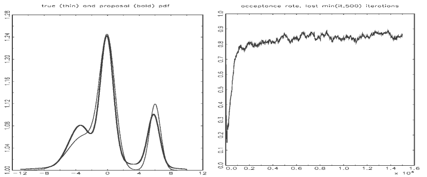
Figure 1: Example 1. Left panel: Proposal distribution (bold) after 15 000 iterations, initialized with a normal $\phi(z;-5,4)$. The target density (thin) is a univariate mixture $0.5\phi(z;0,1)+0.3\phi(z;-3,4)+0.2\phi(z;6,0.5).$ Right panel: Recursive updates of the acceptance rate in the last 500 iterations.

and the initial proposal is $\phi(z;-5,4).$ This proposal has very high importance weights $\pi/g$ in a large part of the support of $z$, but we still quickly converge to a good approximation of the target. Figure 1 shows that the acceptance rates increase fast initially and then stabilize as the proposal distribution also settles down.

The next example shows that as the dimension increases a good initial proposal distribution becomes more valuable.

Example 2 Consider the fifteen dimensional target distribution which is the mixture of two normals

$$\pi(z)=0.7\phi(z;0,I)+0.3\phi(z;\mu_{2},2I),$$

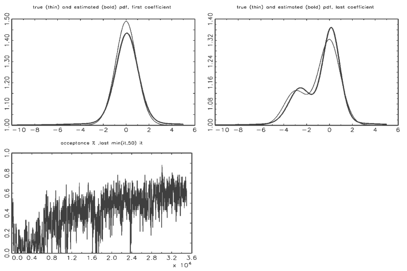
Figure 2: Example 2. Proposal distribution after 35 000 iterations. The target distribution is a 15-dimensional mixture. The graph plots the true marginal distributions (thin) for the first and last variable together with the corresponding marginal distributions (bold) implied by the mixture of normals estimated on the full history of the draws, and with recursive updates of the acceptance rate in the last 500 iterations.

where $\phi(z;\mu,\Sigma)$ is a multivariate normal density with mean $\mu$ and covariance matrix $\Sigma$ evaluated at $z.$ The vector $\mu_{2}$ has elements $\mu_{2,i}=0$ for $i=1,...,14,$ and $\mu_{2,15}=-3.$ The first fourteen marginals are therefore symmetric but slightly leptokurtic, whereas the fifteenth is also skewed. The proposal distribution is initialized by fattening and stretching the tails of the Laplace approximation, that is, a normal distribution centered at the mode and with covariance set to minus the inverse of the Hessian of the log-likelihood at the mode. The Laplace approximation is nearly equal to $\phi(z;0,I)$, so we have $g_{0}(z)\simeq 0.6\phi(z;0,I)+0.4\phi(z;0,16I)$. Figure 2 shows that the acceptance rates at the initial proposal are not high, but sufficient to start the learning process. The AIMH learns the marginal distribution of the non-normal variable rather well and, since most variables are normal, at very low computational cost since we only estimate the mixture parameters on variables that appear skewed. In contrast, an initial proposal such as $\phi(z;m,4I),$ where $m=-5$ generates such low acceptance rates for this fifteen dimensional distribution that the learning process cannot get successfully started.

7 Applications

State space models and nonparametric models are ideal initial applications for AIMH schemes. Although they can have a large number of parameters, it is often the case that, conditional on a small subset, most parameters can be integrated out or have known analytical form. Therefore it is often possible to draw all parameters in one or two blocks. Exploiting these features, it is also often inexpensive to find the posterior mode, possibly for a simplified version of the model, and therefore obtain a reasonable initialization of the proposal distribution. Finally, the standard approach based on Gibbs and Metropolis-within-Gibbs can be very inefficient, particularly for state space models (see Fruhwirth-Schnatter 2004).

For each of our applications we checked the results of the adaptive sampling scheme by re-running the sampler at a number of different starting points using a fixed proposal based on the last mixture in the strict adaptation phase. In all cases we got very similar results to those obtained using strict adaptation.

For our examples we define the inefficiency of a sampling scheme as the factor by which the number of iterates would need to increase to give the same precision (standard error) as a sampler generating independent draws. For two sampling schemes A and B say, we define the inefficiency of scheme B relative to A as the factor by which it is necessary to increase the running time of B in order for it to obtain the same accuracy as A. It is computed as the inefficiency factor of B times its run time per iteration divided by the inefficiency factor of A times its run time per iteration.

In the examples below we compare the performance of the AIMH sampler to the following version of the Haario et al. (2001) adaptive random walk Metropolis sampler proposed on page 3 of Roberts and Rosenthal (2006). Specifically, let $\theta$ be the parameters in the model, $\hat{\theta}$ the posterior mode and $V$ the variance covariance matrix of the Laplace approximation to the posterior. Then at iteration $j$ the proposal distribution is given by

$$Q_{j}(\theta^{c},\cdot) =N(\theta^{c},(0.1)^{2}V/d)\quad\text{ if}\quad j<5d,$$

$$Q_{j}(\theta^{c},\cdot) =(1-\beta)N(\theta^{c},(2.38)^{2}\Sigma_{j}/d)+\beta N(\theta^{c},(0.1)^{2}I_{d}/d)\quad\text{if}\quad j\geq 5d,$$

where $N(\theta,V)$ is the normal density with mean $\theta$ and covariance matrix $V$, $\theta^{c}$ is the current value of $\theta$, $d$ is the dimension of $\theta$, $\beta=0.05$ and $\Sigma_{j}$ is the current empirical estimate of the covariance matrix of the target distribution based on the iterates thus far. In all cases we initialized this sampler at the posterior mode.

7.1 Time-varying parameter autoregressive models

Consider the following time-varying parameter first order autoregressive (AR(1)) process (the extension to a more general autoregressive process is straightforward):

$$y_{t}=c_{t}+\rho_{t}y_{t-1}+\sigma_{\epsilon}\epsilon_{t}\,,\text{ }c_{t}=c_{t-1}+\lambda_{0}\sigma_{\epsilon}u_{t}\text{ and }\rho_{t}=\rho_{t-1}+\lambda_{1}v_{t},$$ (10)

where $\epsilon_{t},u_{t},v_{t}$ are all $nid(0,1).$ The model has three parameters $(\sigma_{\epsilon}^{2},\lambda_{0}^{2},\lambda_{1}^{2}),$ while $c_{0}$ and $\rho_{0}$ can be treated either as parameters or (our choice) as states. Given conjugate priors (inverse gamma for the parameters, and normal for $c_{0}$ and $\rho_{0}$), Gibbs sampling is straightforward (Carter and Kohn 1994). Fruhwirth-Schnatter (2004) reports that based on the autocorrelations of the iterates, Gibbs sampling can be very inefficient for these models. In the following application we also find that the Gibbs draws are highly autocorrelated and, by comparing posterior statistics from Gibbs sampling and from our AIMH, we also find that the autocorrelations do not reveal the full extent of the problem.

7.1.1 Application: US CPI inflation

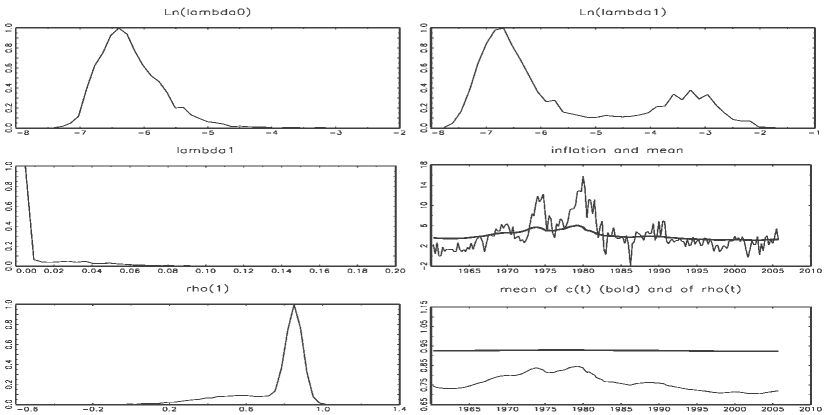
Figure 4: Inference for the model of figure 3 by adaptive IMH. The interpretation of the panels is the same as in figure 3.

We apply the model to quarterly U.S. CPI inflation for the period 1960-2005 (184 observations). We use rather dispersed inverse gamma priors for $\sigma_{\epsilon}^{2},\lambda_{0}^{2},\lambda_{1}^{2}$ with a common shape parameter of 1. The scale parameters are defined by setting the modes of the priors close to maximum likelihood estimates: $\sigma_{OLS}^{2}$ for $\sigma_{\epsilon}^{2}$ (where $\sigma_{OLS}^{2}$ is the residual variance from an AR(1) model estimated by OLS), at $0.01\sigma_{OLS}^{2}$ for $\lambda_{0}^{2}$ and at $0.001^{2}$ for $\lambda_{1}^{2}.$ The modes of $\lambda_{0}^{2}$ and $\lambda_{1}^{2}$ are centered at the maximum likelihood estimates to ensure that the bimodality in the posterior distribution of the log of $\lambda_{1}^{2}$ documented in Figure 4 is not induced by the prior.

For given parameters, the likelihood is easily computed via the Kalman filter. It is therefore simple to find the posterior mode, at which the chain is initialized. Posterior mode values suggest that time variation is nearly absent.

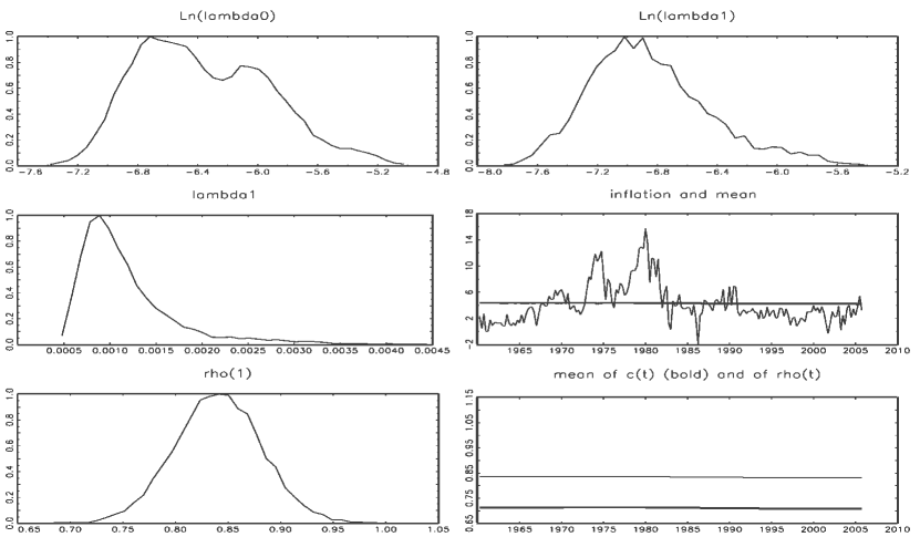
Figure 3: Inference for a time varying parameter AR(1) model for US inflation by Gibbs sampling. (a) marginal distribution of $\ln(\lambda_{0})$ (b) marginal distribution of $\ln(\lambda_{1})$ (c) marginal distribution $\lambda_{1}$ (d) inflation plot and mean, estimated as $E[(c_{t}/1-\rho_{t})|y]$ (e) marginal distribution of $\rho_{0}|y$ (f) $E(c_{t}|y)$ (bold line) and $E(\rho_{t}|y).$

Starting with Gibbs sampling, we draw 40 000 times after a burn-in of 5000. The recursive parameter means seem to settle down (not reported) and the posterior distributions are in line with a normal approximation taken at the mode, suggesting a persistent AR(1) with little sign of parameter variation (see Figure 3). It may therefore seem reasonable to assume that the chain has produced a sample representative of the entire posterior.

However, the AIMH scheme tells a different story. The proposal is initialized at a mixture of two normals $g_{0}(z)=0.5\phi(z;\widehat{\mu},\widehat{\Sigma})+0.5\phi(z;\widehat{\mu},16\widehat{\Sigma})$, where $\widehat{\mu}$ is the posterior mode and $-\widehat{\Sigma}$ is the inverse of the Hessian of the log-posterior evaluated at $\widehat{\mu}$. The AIMH soon discovers that the posterior distribution of $\log(\lambda_{1}^{2}),$ not to mention $\lambda_{1}^{2}$, is highly non-normal (see Figure 4), with substantial probability mass around a second mode corresponding to non-trivial amounts of time variation in $\rho_{t}$ and a lower $\rho_{1}.$

We also ran the adaptive random walk Metropolis sampler outlined at the start of the section. The sampler settles down to an acceptance rate of 20% and obtains the correct posterior distribution, and in particular finds both modes. Table 1 gives the inefficiency factors for all three samplers as well as the inefficiency factors of the Gibbs and ARWM relative to AIMH. The table shows that the AIMH sampler is appreciably more efficient than the other two samplers.

7.2 Additive semiparametric Gaussian models

In this example we consider the additive semiparametric regression model with Gaussian errors, with some of the covariates entering linearly and the others entering more flexibly

$$y_{i}=\sum_{j=1}^{m}\gamma_{j}z_{ji}+\sum_{h=1}^{H}f_{h}(x_{h,i})+\sigma_{\epsilon}\epsilon_{i}\,;$$ (11)

the $\epsilon_{i}$ are $nid(0,1)$ and $z$ is a vector of regressors that enter linearly. The $x_{h},$ $h=1,...,H$ are covariates that enter more flexibly by using the quadratic polynomial spline functions

$$f_{h}(x_{h,i})=\beta_{0,h}x_{h,i}+\sum_{j=1}^{J}\beta_{h,j}(x_{h,i}-\tilde{x}_{h,j})_{+}^{2}=\beta_{0,h}x_{i}+g_{h}(x_{h,i}),$$ (12)

where $x_{+}=x$ if $x>0$ and 0 otherwise and $\{\widetilde{x}_{h,1},...,\widetilde{x}_{h,k}\}$ are points (or ‘knots’) on the abscissae of $x_{h}$ such that $\min(x_{h})=\widetilde{x}_{h,1}<...<\widetilde{x}_{h,J}<\max(x_{h})$. In this paper we choose 30 knots so that each interval contains the same number of observed values of $x_{h}.$ For a discussion of quadratic spline bases and other related bases see chapter 3 of Ruppert et al. (2003). We assume that a global intercept term is included in $z$ in (11) and for simplicity we include the parameters $\beta_{h,0},$ $h=1,\dots,H$ in the vector $\gamma$ and $x_{h},$ $h=1,\dots,H$ as part of the vector $z$. This transforms the nonparametric model into an highly parametrized linear model

$$y=\widetilde{Z}\widetilde{\gamma}+\epsilon.$$ (13)

The prior for the linear parameters $\gamma$ is normal with a diagonal covariance matrix $\gamma\sim N(0,v_{\gamma}^{2}I)$, where $v_{\gamma}$ can be set to a large number. It is also convenient to assume a normal prior for the nonparametric part, with all parameters independent and $\beta_{h,j}\sim N(0,\tau_{h}^{2}),\ ,j=1,...,J,\,h=1,...,H.$ However, with this prior there is a high risk of over-fitting if we simply set $\tau_{h}^{2}$ to a large number. The variance $\tau_{h}^{2}$ is often chosen by cross-validation, but in a fully Bayesian setting we can treat $\tau_{h}^{2}$ as a parameter. To illustrate the advantage of AIMH in working with different priors, we experiment with two options for the prior $\tau_{h}^{2}$. The first prior is log-normal and rather dispersed: $\ln(\tau_{h}^{2})\sim N(0,5^{2})$, the second is inverse gamma with shape parameter 1 and scale parameter implied by setting the mode at $0.1^{2}$. The prior for $\sigma_{\epsilon}^{2}$ is inverse gamma with shape parameter one and scale parameter implied by setting the prior mode at the OLS residual variance estimated on (13). The prior for $\widetilde{\gamma}=(\gamma,\beta_{1},...,\beta_{H})$ is therefore jointly normal conditional on $\tau^{2}=\{\tau_{1}^{2},..,\tau_{H}^{2}\}$, $\widetilde{\gamma}|\tau\sim N(\mathbf{0},V_{\widetilde{\gamma}}(\tau))$, where $V_{\widetilde{\gamma}}(\tau)=\text{diag}(v_{\gamma}^{2}I,\tau_{1}^{2},I,\dots,\tau_{H}^{2}I)$ is a block diagonal matrix. One way to estimate the posterior density of the semiparametric model is to use Gibbs or Metropolis-within-Gibbs sampling as proposed by Wong and Kohn (1996). In this approach the parameters $\widetilde{\gamma}=\{\gamma,\beta_{1},...,\beta_{H}\}$ are conjugate given $\theta=\{\sigma_{\epsilon}^{2},\tau_{1}^{2},...,\tau_{H}^{2}\},$ and $\sigma_{\epsilon}^{2}$ is conjugate given $\widetilde{\gamma}.$ Each variance $\tau_{h}^{2}$ can be updated with a Gibbs step for the inverse gamma prior, or with a Metropolis-Hastings step for the log-normal prior. In this second case, we use a Laplace approximation of $p(\ln(\tau_{h}^{2})|\beta_{h})$, which is very fast to compute using analytical derivatives. However, the correlation between $\tau_{h}^{2}$ and $\{\beta_{h,1},..,\beta_{h,J}\}$ could be quite high using either prior for $\tau_{h}^{2}$. In addition, using a log normal prior for $\tau_{h}^{2}$ leads to high rejection rates in the Metropolis-Hastings step when generating the $\tau_{h}^{2}$. Both problems are elegantly solved by integrating out $\widetilde{\gamma}$ and generating $\theta$ as a block using an efficient AIMH sampler.

The next example shows how to update all parameters in one block with an efficient AIMH sampler. We first note that, conditional on $\theta$, $\widetilde{\gamma}$ can be integrated out, making it possible to compute $p(\theta|y)\propto p(y|\theta)p(\theta),$ where $y|\theta\sim N(\mathbf{0},\sigma_{\epsilon}^{2}I+\widetilde{Z}V_{\widetilde{\gamma}}(\tau)\widetilde{Z}^{\prime})$.

7.2.1
Application: Boston housing data

We use the Gaussian semiparametric model to study the Boston housing data introduced by Harrison and Rubinfield (1978) and analyzed semiparametrically by Smith and Kohn (1996). There are 506 observations. The dependent variable is the log of $MV$, the median value of owner-occupied homes. We use all 13 available covariates (see Smith and Kohn or the web-site for a full description) in the linear part and the following six in the nonparametric part (Smith and Kohn use only the first five): $X_{5}=NOX$, nitrogen oxide concentration, $X_{6}=RM,$ average number of rooms, $X_{8}=DIS,$ logarithm of the distance from five employment centers, $X_{10}=TAX,$ property tax rate, $X_{13}=STAT,$ proportion of the population that is lower status, $X_{1}=CRIM,$ per capita crime rate by town.

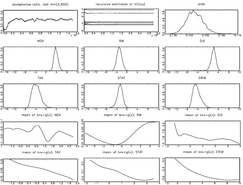
Figure 5: Inference for semiparametric model of housing prices by adaptive IMH. First row: recursive acceptance rate for the last min(it,500) iterations, recursive means of $\ln(\tau_{i}),$ marginal of $\sigma_{\epsilon}.$ Second and third rows: marginals of $\ln(\tau_{i}).$ Fourth and fifth rows: means of $\beta_{i}x+g_{i}(x).$

The proposal distribution for the seven parameters $\theta=\{\ln(\sigma_{\epsilon}^{2}),\ln(\tau_{5}^{2}),...,\allowbreak\ln(\tau_{1}^{2})\}$ is initialized by fattening the tails of the Laplace approximation. To find the Laplace approximation, we simply apply Newton-Raphson optimization (with numerical derivatives) to $\ln p(y|\theta)+\ln p(\theta),$ which involves no extra coding effort since both densities are needed to compute the MH acceptance ratio. Figure 5 provides results for the case of a log-normal prior on $\tau_{h}^{2},$ $h=1,...,H$ and shows that the acceptance rate quickly improves and stabilizes at around 60% when all seven parameters are updated jointly. Most parameters are approximately lognormally distributed, except those connected to the variables $TAX$ and $CRIM$, which benefit from the added flexibility of mixtures. The correlation matrix of the smoothing parameters $\{\ln(\tau_{5}^{2}),...,\ln(\tau_{1}^{2})\}$ is nearly diagonal. This suggests that the AIMH could handle large numbers of smoothing parameters efficiently by updating them in blocks (with a different proposal density estimated adaptively on each block), since the blocks would be nearly independent of each other.

Table 1 reports the inefficiency factors for both the Gibbs sampler and the AIMH sampler for both inverse gamma and log normal priors, as well as the inefficiency of the Gibbs sampler relative to the AIMH sampler. The table shows that in terms of relative efficiency (defined at the beginning of section 7), the AIMH is about 40% more efficient than the Gibbs sampler when both samplers use the inverse gamma prior on $\tau_{h}^{2}$, and nearly seven times more efficient when both samplers use the log-normal prior. Reported results are for the average inefficiency factors (over both $h$ and $i$) of $f_{h}(x_{h,i})$. Looking at the autocorrelation of the log-parameters gives similar inefficiency ratios.

We also applied the adaptive random walk Metropolis sampler to this data set, but could not make it work well. With the sampler initialized at the posterior mode, the acceptance rate started at over 50%, but within a few hundred iterations fell to below 1% and stayed there indefinitely. We do not report any inefficiency factors for this sampler because we do not believe that inference is reliable with such a low acceptance rate. We conjecture that the poor behavior of the ARWM sampler in this example compared to the other two examples is because this example has 7 parameters whereas the other two have 3 and 2 parameters. In addition, the second derivatives of the log posterior in this example are far from constant, so a unique covariance matrix may do very poorly. By contrast, a mixture of normals allows for local correlations between the parameter and therefore may be less affected.

Boston	mean $f_{h}(x_{h,i})$		Inflation	$\log(\sigma_{\epsilon}^{2})$	$\log$($\lambda_{0}^{2})$	$\log$($\lambda_{1}^{2})$
AIMH, IG	2.6		AIMH	6.7	2.8	6.1
Gibbs, IG	6.3 (1.4)		Gibbs	9.4 (1.3)	113.3 (37.4)	156.4 (23.7)
AIMH, LN	1.6 (6.8)		ARWM	21.5 (3.1)	23.5 (8.3)	23.6 (3.8)
M-Gibbs, LN	18.4

Table 1: Inefficiency factors for the semiparametric (Boston) and state space (inflation) models, together with the inefficiencies of the Gibbs sampler and the ARWM relative to the AIMH sampler in brackets. AIMH: adaptive independent Metropolis-Hastings; M-Gibbs: Metropolis-within-Gibbs; and ARWM: adaptive random walk Metropolis. IG and LN: inverse gamma and log-normal priors for the Boston data.

7.3 Stochastic volatility models

The simplest stochastic volatility model can be written for mean corrected data as

$$y_{t}=e^{0.5h_{t}}\epsilon_{t}\,,\text{ }h_{t}=\mu+\rho(h_{t-1}-\mu)+\sigma v_{t},$$ (14)

where $\epsilon_{t}$ is $nid(0,1)$ and the model parameters are $\theta=\{\mu,\rho,\sigma\}.$ We square and take logs of the observation equation, and we approximate the distribution of $\ln(\epsilon_{t}^{2}),$ which is the log of a chi-squared 1, by a mixture of normals as in Kim et al. (1998). This model has a conditionally Gaussian state space form

$$\widetilde{y}_{t}=g(K_{t})+h_{t}+G(K_{t})u_{t}\,,\text{ }h_{t}=\mu+\rho(h_{t-1}-\mu)+\sigma v_{t},$$ (15)

where $\epsilon_{t}$ is $nid(0,1),$ $\widetilde{y}_{t}=$ $\ln(y_{t}^{2}),$ and $g(K_{t})$ and $G(K_{t})$ are known given $K_{t}$.

The indicators $K$ can be sampled in one block given $\theta$ and $h$ as in Carter and Kohn (1994). The distribution of $\theta$ given $h$ is conjugate, but Kim et al. (1998) show that $\theta$ and $h$ are highly correlated and recommend drawing $\theta$ given $y$ and $K$ but integrating $h$ out. This is accomplished with a Metropolis-Hastings step, where $p(y|K,\theta)$ is computed via the Kalman filter. Since the posterior mode is not readily available, Kim et al. (1998) use IMH, where the proposal distribution is calibrated once from draws obtained with a less efficient sampling scheme. This is less efficient than our scheme and requires coding two different samplers. An alternative we now explore is to use AIMH from the beginning of the chain.

7.3.1 Application: USD-GBP daily returns

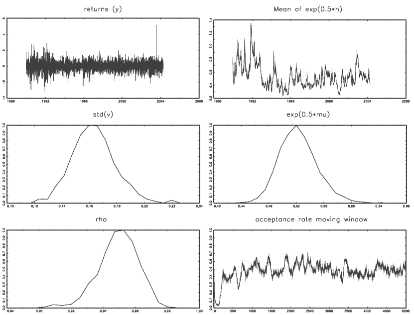
Figure 6: Inference for the daily US-GBP exchange rate by AIMH. (a) exchange rate returns (b) mean of $0.5\ln(h_{t})$ (c) marginal of $\sigma_{v}$ (d) marginal of $0.5\exp(\mu)$ (e) marginal of $\rho$ (f) moving window of the acceptance rate for the last min(it,500) iterations.

We analyze daily U.S. dollar - British pound returns (defined as the first difference of the log of the nominal exchange rate) for the period January 1990 to March 2004. The parameter $\mu$ can be integrated out (see Kim et al. (1998)). To initialize the proposal distribution, we approximate the distribution of $\ln(\epsilon_{t}^{2})$ as a normal with mean $-1.27$ and variance $2.22^{2}$. This gives a standard Gaussian state space model, for which the Laplace approximation is easily available. We also use the mode to center the priors for $\rho$ and $\ln(\sigma^{2})$, which are normal and dispersed. The prior for $\rho$ is truncated at 1. With fattened tails, the initial proposal gives an acceptance rate of around 10%, and Figure 6 shows that it takes only a few hundred iterations for the acceptance rates to increase to around 50%. This number is satisfactory given that the proposal approximates $p(\theta|y)$ while the acceptance probability is computed on $p(\theta|y,K)$.

The adaptive random walk Metropolis sampler also quickly settled down to an acceptance rate of around 15%, with the chain mixing well. The inefficiency factors for $\rho$ and $\sigma^{2}$ for both samplers are given in table 2, together with the inefficiency factors for the adaptive random walk Metropolis relative to AIMH. The table shows that AIMH compares favourably with ARWM.

Sampling Scheme	$\rho$	$\sigma^{2}$
AIMH	7.6	9.2
ARWM	21.1 (2.7)	26.5 (2.86)

Table 2: Inefficiency factors for the stochastic volatility model for the adaptive independent Metropolis-Hastings (AIMH) sampler and the adaptive random walk Metropolis (ARWM) sampler, with the relative inefficiency of the AWRM in brackets.

8 Conclusion

This paper shows that it is possible to build adaptive independent Metropolis-Hastings samplers that can do better than two-step adaptation because they adapt throughout the sampling period. The most interesting applications arise when current best practice is inefficient or cumbersome and, in our opinion, when adaptation starts early. Our article provides a fast and reliable algorithm which performs well in three interesting models and compares favorably on these examples with a standard Markov chain Monte Carlo sampler and an adaptive random walk Metropolis sampler.

Appendix 1: k-harmonic means clustering

We estimate the mixture of normal parameters using the k-harmonic means clustering algorithm which can be described as follows. (See Hamerly and Elkan 2002, for a discussion). Let $p$ be the number of clusters.

1. Initialize the algorithm with $c_{1},...,c_{p},$ the component centers. The starting values are chosen with the procedure of Bradly and Fayyad (1998) . We depart slightly from Bradley and Fayyad in using the harmonic k-means algorithm (rather than k-means) in the initialization procedure.

2. For each data point $\theta_{t},$ compute a weight function $w(\theta_{t})$ and a membership function $m(c_{i}|\theta_{t})$ for $t=1,...,p$ as

   $$w(\theta_{t})=\frac{\sum_{i=1}^{p}||\theta_{t}-c_{i}||^{-p-2}}{(\sum_{i=1}^{p}||\theta_{t}-c_{i}||^{-p})^{2}}\quad\text{and}\quad m(c_{i}|\theta_{t})=\frac{||\theta_{t}-c_{i}||^{-p-2}}{\sum_{i=1}^{p}||\theta_{t}-c_{i}||^{-p-2}},$$

   where $||\theta_{t}-c_{i}||$ is the Euclidean or Mahalanobis distance. Following Bradly and Fayyad (1998), we put a lower boundary $\epsilon$ on $||\theta_{t}-c_{i}||$ (to avoid degeneracies when trying $||c_{i}-c_{i}||$). The membership function softens the sharp membership of the k-means algorithm, so one observation can belong to more than one cluster in differing degrees. The weight function gives more weight to observations that are currently covered poorly (i.e. that are far from the nearest center).

3. Update each center $c_{i}$

   $$c_{i}=\frac{\sum_{t=1}^{n}m(c_{i}|\theta_{t})w(\theta_{t})\theta_{t}}{\sum_{t=1}^{n}m(c_{i}|\theta_{t})w(\theta_{t})}.$$

4. Repeat until convergence. This gives the cluster centers, which we take as estimates of the component means. The other mixture parameters can then be estimated for $i=1,...,k$ as

   $$V_{i}=\frac{\sum_{t=1}^{n}m(c_{i}|\theta_{t})w(\theta_{t})(\theta_{t}-c_{i})(\theta_{t}-c_{i})^{\prime}}{\sum_{t=1}^{n}m(c_{i}|\theta_{t})w(\theta_{t})}\quad\text{and}\quad\pi_{i}\varpropto\sum_{t=1}^{n}m(c_{i}|\theta_{t})w(\theta_{t}).$$

5. The number of clusters is chosen with the BIC criterion given a maximum number (5 in our examples).

We notice that the covariance matrices $V_{i}$ are only estimated once, after convergence. k-means type algorithms also differ from the EM algorithm in that they do not evaluate the likelihood $p(\theta|c_{1},...,\pi_{1,}V_{1},...)$. This sub-optimal use of information in fact turns out to be a great advantage for our purposes. Fewer iterations than for EM are needed for convergence, and each iteration is faster. Even more importantly, the algorithm does not get stuck in the small degenerate clusters caused by rejections in the sense that, unlike for the EM algorithm with freely estimated covariances, these small clusters are not absorbing. If k-harmonic means does find a degenerate cluster, this causes no trouble for convergence, and after convergence we can use a predefined matrix in place of any non-positive-definite covariance matrix (for example, if $V_{i}$ is not positive definite we set it to $0.5^{2}Var(\theta)$). If desired, the mixture parameters can be refined with a few steps of the EM algorithm. In this case, we recommend not updating the the covariance matrices for the reasons just discussed.

Appendix 2: Proofs

The one-step transition kernel for $Z_{n+1}$ in section 3 is given by

$$T_{n}(z,dz^{\prime}) =\alpha_{n}(z,z^{\prime})q_{n}(z^{\prime})\mu\{dz^{\prime}\}+\delta_{z}(dz^{\prime})(1-\nu_{n}(z))$$ (16)

where $\delta_{z}(dz^{\prime})=1$ if $z\in dz^{\prime}$ and is 0 otherwise, and

$$\nu_{n}(z)=\int_{\cal Z}\alpha_{n}(z,z^{\prime})q_{n}(z^{\prime})\mu\{dz^{\prime}\}.$$ (17)

By the construction of the MH transition kernel,

$$\quad\int_{\cal Z}\pi(z)T_{n}(z,dz^{\prime})\mu\{dz\} =\pi(z^{\prime})\mu\{dz^{\prime}\}\ .$$ (18)

In this section $K$ is a generic constant, independent of $n,z$ and $z^{\prime}$. It is convenient to write $h_{n}(z;\lambda_{n})$ as $h_{n}(z)$ Without loss of generality we assume throughout this section that $\cal Z$ is a discrete space. Exactly the same proof goes through for the continuous case with summations replaced by integrals. We use the notation $z_{s:t}$ to mean $\{z_{s},\dots,z_{t}\}$ for $s\leq t$, with a similar interpretation for $Z_{s:t}$.

To prove Theorem 1 we first obtain the following two lemmas.

Lemma 1

Under the assumptions of Section 2, for any $n,k>0$ and $z,z^{\prime}\in\cal Z$,
(a) $q_{n}(z)\leq Kg_{0}(z)$.
(b) $\alpha_{n}(z,z^{\prime})q_{n}(z^{\prime})\leq Kg_{0}(z^{\prime})$
(c) There exists an $\epsilon_{1}$, $0<\epsilon_{1}<1$, such that $\alpha_{n}(z,z^{\prime})q_{n}(z^{\prime})>\epsilon_{1}\pi(z^{\prime})$ for all $z,z^{\prime}\in\cal Z$.
(d) $\nu_{n}(z)>\epsilon_{1}$ for all $z\in\cal Z$, where $\nu_{n}(z)$ is defined by (17).
(e) For $k\geq 1$, let $\Delta_{n}(z,z^{\prime})=\alpha_{n}(z,z^{\prime})q_{n}(z^{\prime})-\alpha_{n+1}(z,z^{\prime})q_{n+1}(z^{\prime})$. Then,

$$\mid\Delta_{n}(z,z^{\prime})\mid\ \leq\ K\biggl{(}g_{0}(z^{\prime})+\frac{\pi(z^{\prime})}{\pi(z)}g_{0}(z)\biggr{)}a_{n}.$$ (19)

(f)

$$\mid\nu_{n}(z)-\nu_{n+1}z)\mid\leq K\biggl{(}1+\frac{g_{0}(z}{\pi(z)}\biggr{)}a_{n}$$ (20)

Proof. (a) $q_{n}(z)/g_{0}(z)=\omega_{1}+(1-\omega_{1})\bar{g}_{n}(z)/g_{0}(z)$ and the result follows from (3). (b) follows from (a) and $\alpha_{n}(z,z^{\prime})\leq 1$. To show (c), note that $q_{n}(z)/\pi(z)\geq\omega_{1}g_{0}(z)/\pi(z)$. From (3), there is an $\epsilon_{1}$ such that $q_{n}(z)/\pi(z)>\epsilon_{1}$ for all $z\in\cal Z$. It is now straightforward to show that $\alpha_{n}(z,z^{\prime})q_{n}(z^{\prime})/\pi(z^{\prime})>\epsilon_{1}$ for all $z,z^{\prime}\in\cal Z$. (d) follows from

$$\nu(z) =\sum_{z^{\prime}}\alpha_{n}(z,z^{\prime})q_{n}(z^{\prime})>\epsilon_{1}\sum_{z^{\prime}}\pi(z^{\prime})=\epsilon_{1}$$

To obtain (e), it is necessary to consider the following four cases.

Case 1. $\alpha_{n}(z,z^{\prime})=1$ and $\alpha_{n+1}(z,z^{\prime})=1$. Then, $|\Delta_{n}|=\mid q_{n}(z^{\prime})-q_{n+1}(z^{\prime})\mid\ \leq\ Kg_{0}(z^{\prime})a_{n}$ by (4).

Case 2. $\alpha_{n}(z,z^{\prime})<1$ and $\alpha_{n+1}(z,z^{\prime})<1$.

$$\mid\Delta_{n}(z,z^{\prime})\mid =\frac{\pi(z^{\prime})}{\pi(z)}\mid q_{n}(z)-q_{n+1}(z)\mid\ \leq\ K\frac{\pi(z^{\prime})}{\pi(z)}g_{0}(z)a_{n}.$$

Case 3. $\alpha_{n}(z,z^{\prime})=1$ and $\alpha_{n+1}(z,z^{\prime})<1$. In this case $\Delta_{n}(z,z^{\prime})=q_{n}(z^{\prime})-\pi(z^{\prime})q_{n+1}(z)/\pi(z)$. If $\Delta_{n}(z,z^{\prime})\geq 0$, then

$$0\leq\Delta_{n}(z,z^{\prime})\leq\frac{\pi(z^{\prime})}{\pi(z)}\biggl{(}q_{n}(z)-q_{n+1}(z)\biggr{)}\leq Kg_{0}(z)a_{n}c_{k}\ .$$

If $\Delta_{n}(z,z^{\prime})<0$, then

$$0<-\Delta_{n}(z,z^{\prime})=\frac{\pi(z^{\prime})}{\pi(z)}q_{n+1}(z)-q_{n}(z^{\prime})\leq q_{n+1}(z^{\prime})-q_{n}(z^{\prime})$$

Thus,

$$\mid\Delta_{n}(z,z^{\prime})\mid\ \leq\ K\biggl{(}g_{0}(z^{\prime})+\frac{\pi(z^{\prime})}{\pi(z)}\biggr{)}a_{n}.$$

Case 4. $\alpha_{n}(z,z^{\prime})<1$ and $\alpha_{n+1}(z,z^{\prime})=1$. This case is similar to case 3.

To obtain (f), we note that

$$\mid\nu_{n}(z)-\nu_{n+1}(z)\mid\ \leq\ \sum_{z^{\prime}}|\Delta_{n}(z,z^{\prime})|\ ,$$

and the result follows from (e).   

With $\epsilon_{1}$ as in Lemma 1, choose $0<\epsilon<\epsilon_{1}$ and let

$$R_{n}(z,z^{\prime}) =\frac{T_{n}(z,z^{\prime})-\epsilon\pi(z^{\prime})}{1-\epsilon}$$ (21)

Then, $R_{n}(z,z^{\prime})$ is a one-step transition kernel with the following properties.

Lemma 2

(a)

$$\sum_{z}\pi(z)R_{n}(z,z^{\prime}) =\pi(z^{\prime})\ .$$

(b)

$$R_{n}(z,z^{\prime}) \leq Kg_{0}(z_{n})+\eta\delta_{z}(z^{\prime})$$

where $0<\eta<1$.
(c)

$$\mid R_{n}(z,z^{\prime})-R_{n+1}(z,z^{\prime})\mid\ \leq\ Ka_{n}\biggl{\{}\biggl{(}g_{0}(z^{\prime})+\frac{\pi(z^{\prime})}{\pi(z)}g_{0}(z)\biggr{)}+\biggl{(}1+\frac{g_{0}(z)}{\pi(z)}\biggr{)}\delta_{z}(z^{\prime})\biggr{\}}$$

(d)

$$\sum_{z_{n-m+1}}\cdots\sum_{z_{n-1}}\prod_{k=1}^{m}R_{n-k}(z_{n-k},z_{n-k+1}) \leq Kg_{0}(z_{n})+\eta^{m}\delta_{z_{n-m}}(z_{n})$$

(e) For $1\leq l\leq j-1$ and $j=1,\dots,n$,

$$\sum_{z_{n-l-1}}\cdots\sum_{z_{n-j+1}}\pi(z_{n-j+1})\prod_{k=1+1}^{j-1}R_{n-j}(z_{n-k},z_{n-k+1}) =\pi(z_{n-l})$$

(f) For $j=1,\dots,n$ and $l=1,\dots,j-1$,

$$\mid\sum_{z_{n-j+1}}\cdots\sum_{z_{n-1}}\pi(z_{n-j+1})\prod_{k=l+1}^{j-1}R_{n-j}(z_{n-k},z_{n-k+1})$$

$$\times\biggl{(}R_{n-l}(z_{n-l},z_{n-l+1})-R_{n-j}(z_{n-l},z_{n-l+1})\biggr{)}\prod_{k=1}^{l-1}R_{n-k}(z_{n-k},z_{n-k+1})\mid \ \leq\ Kg_{0}(z_{n})a_{n-j}(j-l)^{-1}$$

Proof. (a) follows from (21) and (18). (b) follows from (21). (c) follows from (19) and (20). (d) is true for $m=1$ and is obtained in general by induction. (e) follows from part (a). (f) follows from parts (a) to (e).   

Proof of Theorem 1. Let $\Delta_{j},j=1,2,\dots$ be an independent Bernoulli process such that $\Delta_{j}=1$ with probability $\epsilon$ and $\Delta_{j}=0$ with probability $1-\epsilon$. From (21), $T_{n}(z,z^{\prime})=(1-\epsilon)R_{n}(z,z^{\prime})+\epsilon\pi(z^{\prime})$ so that we can interpret $T_{n}(z,z^{\prime})$ as a mixture of transition kernels, such that $T_{n}(z,z^{\prime})=R_{n}(z,z^{\prime})$ if $\Delta_{n}=0$ and $T_{n}(z,z^{\prime})=\pi(z^{\prime})$ if $\Delta_{n}=1$. For $j=1,\dots,n$, let $A_{n,j}$ be the event that $\Delta_{n-j+1}=1,\Delta_{k}=0,k=n-j+2,\dots,n$. Let $B_{n}$ be the event that $\Delta_{j}=0$ for $j=1,\dots,n$. Then $\Pr(A_{n,j})=\epsilon(1-\epsilon)^{j-1}$ and $\Pr(B_{n})=(1-\epsilon)^{n}$, and

$$\Pr(Z_{n}=z_{n}) =\sum_{j=1}^{n}\Pr(Z_{n}=z_{n}\mid A_{n,j})\Pr(A_{n,j})+\Pr(Z_{n}=z_{n}\mid B_{n})\Pr(B_{n}).$$

As in the proof of Theorem 1 in Nott and Kohn (2005), we can write $\Pr(Z_{n}=z_{n}|A_{n,j})=C_{0,j}+C_{1,j}+\cdots+C_{j-1,j}$, where

$$C_{l,j} =\sum_{z_{0}}\cdots\sum_{z_{n-1}}\Pr(Z_{0:n-j}=z_{0:n-j})\pi(z_{n-j+1})\prod_{k=l+1}^{j-1}R_{n-j}(z_{n-k},z_{n-k+1})$$

$$\biggl{(}R_{n-l}(z_{n-l},z_{n-l+1})-R_{n-j}(z_{n-l},z_{n-l+1})\biggr{)}\prod_{k=1}^{l-1}R_{n-k}(z_{n-k},z_{n-k+1})$$

From part (e) of Lemma 2, $C_{0,j}=\pi(z_{n})$ and by part (f) of Lemma 2, $\mid C_{j,n}\mid\leq Kg_{0}(z_{n})a_{n-j}(j-l)^{-1}$ for $j>1$. Using a similar argument to that in Nott and Kohn (2005), this implies that

$$\biggl{|}\sum_{l=0}^{j-1}C_{l,j}\biggr{|} \leq\pi(z_{n})+Kg_{0}(z_{n})(n-j)^{-r_{1}}j^{2}\ .$$

Thus,

$$\sum_{j=1}^{n}\Pr(Z_{n}=z_{n}|A_{n,j})\Pr(A_{n,j})=\pi(z_{n})-(1-\epsilon)^{n}\pi(z_{n})+\eta_{n}\quad\text{where}$$

$$\mid\eta_{n}\mid\ \leq\ Kn^{-r_{1}}\sum_{j=1}^{n-1}\biggl{(}1-\frac{j}{n}\biggr{)}^{-r_{1}}j^{2}\epsilon(1-\epsilon)^{j-1}.$$

We also have that

$$\Pr(Z_{n}=z_{n}\mid B_{n}) =\sum_{z_{0}}\cdots\sum_{z_{n-1}}q_{I}(z_{0})q_{I}(z_{1})\prod_{k=1}^{n-1}R_{k}(z_{k},z_{k+1})$$

$$\leq Kg_{0}(z_{n})+\eta^{n-1}q_{I}(z_{n})\leq Kg_{0}(z_{n})\ .$$

using Lemma 2 (c) and (3). Hence,

$$\mid\Pr(Z_{n}=z_{n})-\pi(z_{n})\mid\ \leq\ Kg_{0}(z_{n})\biggl{(}(1-\epsilon)^{n}+n^{-r_{1}}\biggr{)}$$ (22)

The proof of Theorem 1 follows.   

The proof of Theorem 2 is similar to that in Nott and Kohn (2005) if we use (22).

References

- Andrieu and Moulines (2006) Andrieu, C. and Moulines, D. (2006), “On the ergodicity properties of some adaptive MCMC algorithms,” Annals of Applied Probability, 16, 1462–1505.
- Andrieu et al. (2005) Andrieu, C., Moulines, D., and Doucet, A. (2005), “Stability of stochastic approximation under verifiable conditions,” SICON, 44, 283–312.
- Andrieu and Robert (2001) Andrieu, C. and Robert, C. P. (2001), “Controlled MCMC for optimal sampling,” Technical report, University of Bristol.
- Atchadé and Rosenthal (2005) Atchadé, Y. and Rosenthal, J. (2005), “On adaptive Markov chain Monte Carlo algorithms,” Bernoulli, 11, 815–828.
- Bradly and Fayyad (1998) Bradly, P. and Fayyad, U. (1998), “Refining initial points for k-means clustering,” Proceedings of the 15th International Conference on Machine Learning, 91–99.
- Carter and Kohn (1994) Carter, C. and Kohn, R. (1994), “On Gibbs sampling for state-space models,” Biometrika, 83, 589–601.
- Figuereido and Jain (2002) Figuereido, M. and Jain, A. (2002), “Unsupervised learning of finite mixture models,” IEEE Transactions on Pattern Analysis and Machine Intelligence, 24, 381–396.
- Fruhwirth-Schnatter (2004) Fruhwirth-Schnatter, S. (2004), “Efficient Bayesian parameter estimation,” in State space and unobserved component models, eds. Harvey, A., Koopman, S., and Shephard, N., Cambridge: Cambridge University Press, pp. 123–151.
- Gåsemyr (2003) Gåsemyr, J. (2003), “On an adaptive version of the Metropolis-Hastings algorithm with independent proposal distribution,” Scandinavian Journal of Statistics, 30, 159–173.
- Gelman and Rubin (1992) Gelman, A. and Rubin, D. B. (1992), “Inference from iterative simulation using multiple sequences,” Statistical Science, 7, 473–83.
- Gilks et al. (1998) Gilks, W., Roberts, G., and Sahu, S. (1998), “Adaptive Markov chain Monte Carlo through regeneration,” Journal of the American Statistical Association, 93, 1045–1054.
- Giordani and Kohn (2008) Giordani, P. and Kohn, R. (2008), “Efficient Bayesian inference for multiple change-point and mixture innovation models,” Journal of Business and Economic Statistics, 26, 66–77.
- Haario et al. (2001) Haario, H., Saksman, E., and Tamminen, J. (2001), “An adaptive Metropolis algorithm,” Bernoulli, 7, 223–242.
- Hamerly and Elkan (2002) Hamerly, G. and Elkan, C. (2002), “Alternatives to the k-means algorithm that find better clusterings,” in Proceedings of the Eleventh International Conference on Information and Knowledge Management, eds. Kalpakis, K., Goharian, N., and Grossmann, D., New York: Academic Press, pp. 600–607.
- Harrison and Rubinfield (1978) Harrison, D. and Rubinfield, D. (1978), “Hedonic prices and the demand for clean air,” Journal of Environmental Economics and Management, 5, 81–102.
- Hastie (2005) Hastie, D. (2005), “Towards automatic reversible jump Markov chain Monte Carlo,” Unpublished PhD dissertation, Department of Mathematics, University of Bristol.
- Hastings (1970) Hastings, W. (1970), “Monte Carlo sampling methods using Markov chains and their applications,” Biometrika, 57, 97–109.
- Hesterberg (1998) Hesterberg, T. C. (1998), “Weighted average importance sampling and defensive mixture distributions,” Technometrics, 37, 185–194.
- Holden (1998) Holden, L. (1998), “Adaptive chains,” Manuscript, Norwegian Computing Center, Oslo.
- Kim et al. (1998) Kim, S., Shepherd, N., and Chib, S. (1998), “Stochastic volatility: likelihood inference and comparison with ARCH models,” Review of Economic Studies, 65, 361–394.
- McLachlan and Peel (2000) McLachlan, G. and Peel, D. (2000), Finite Mixture Models, New York: Wiley.
- Mengersen and Tweedie (1996) Mengersen, K. L. and Tweedie, R. L. (1996), “Rates of convergence of the Hastings and Metropolis algorithms,” The Annals of Statistics, 24, 101–21.
- Metropolis et al. (1953) Metropolis, N., Rosenbluth, A. W., Rosenbluth, M. N., H., T. A., and Teller, E. (1953), “Equation of state calculations by fast computing machines,” Journal of Chemical Physics, 21, 1087–1092.
- Nott and Kohn (2005) Nott, D. and Kohn, R. (2005), “Adaptive sampling for Bayesian variable selection,” Biometrika, 92, 747–763.
- Roberts and Rosenthal (2006) Roberts, G. O. and Rosenthal, J. S. (2006), “Examples of adaptive MCMC,” Preprint (http://probability.ca/jeff/ftpdir/adaptex.pdf).
- Roberts and Rosenthal (2007) — (2007), “Coupling and ergodicity of adaptive MCMC,” Journal of Applied Probability, 44, 458–475.
- Ruppert et al. (2003) Ruppert, D., Wand, M., , and Carroll, R. (2003), Semiparametric regression, Cambridge: Cambridge University Press.
- Smith and Kohn (1996) Smith, M. and Kohn, R. (1996), “Nonparametric regression using Bayesian variable selection,” Journal of Econometrics, 75, 317–343.
- Spall (2003) Spall, J. (2003), Introduction to Stochastic Search and Optimization, New York: Wiley.
- Ueda et al. (2000) Ueda, N., Nakano, R., Ghahramani, Z., and Hinton, G. (2000), “SMEM algorithm for mixture models,” Neural Computation, 12, 2109–2128.
- Verbeek et al. (2003) Verbeek, J., Vlassis, N., and Krose, B. (2003), “Efficient Greedy Learning of Gaussian Mixture Models,” Neural Computation, 15, 469–485.
- Wong and Kohn (1996) Wong, C. and Kohn, R. (1996), “A Bayesian approach to additive semiparametric regression,” Journal of Econometrics, 74, 209–235.