Convexity properties of Thompson’s group $F$

Abstract.

We prove that Thompson’s group $F$ is not minimally almost convex with respect to any generating set which is a subset of the standard infinite generating set for $F$ and which contains $x_{1}$. We use this to show that $F$ is not almost convex with respect to any generating set which is a subset of the standard infinite generating set, generalizing results in [HST].

1. Introduction

Convexity properties of a group $G$ with respect to a finite generating set $S$ yield information about the configuration of spheres within the Cayley graph $\Gamma(G,S)$ of $G$ with respect to $S$. A finitely generated group $G$ is almost convex(k), or $AC(k)$ with respect to a finite generating set $X$ if there is a constant $L(k)$ satisfying the following property. For every positive integer $n$, any two elements $x$ and $y$ in the ball $B(n)$ of radius $n$ with $d_{X}(x,y)\leq k$ can be connected by a path of length $L(k)$ which lies completely within this ball. J. Cannon, who introduced this property in [C], proved that if a group $G$ is $AC(2)$ with respect to a generating set $X$ then it is also $AC(k)$ for all $k\geq 2$ with respect to that generating set. Thus if $(G,X)$ is $AC(2)$, it is called almost convex with respect to that generating set.

Almost convexity is a property which depends on generating set; this was proven by C. Thiel using the generalized Heisenberg groups [T]. If a group is almost convex with respect to any generating set, then we simply call it almost convex, omitting the mention of a generating set. Groups which are almost convex with respect to any generating set include hyperbolic groups [C] and fundamental groups of closed 3-manifolds whose geometry is not modeled on Sol [SS]. Moreover, amalgamated products of almost convex groups retain this property [C].

If $(G,X)$ is not almost convex then there is a sequence of points $\{x_{i},y_{i}\}$ at distance $2$ in $B(n_{i})$ which require successively longer paths within $B(n_{i})$ to connect them, as $i$ and $n_{i}$ increase. Such groups include include fundamental groups of closed 3-manifolds whose geometry is modeled on Sol [CFGT] and the solvable Baumslag-Solitar groups $BS(1,n)$ [MS], in both cases with respect to any finite generating set, and Thompson’s group $F$ with respect to any generating set of the form $\{x_{0},x_{1},\ldots,x_{n}\}$ which is a subset of the standard infinite generating set for $F$ [CT1, HST].

Clearly, any two points in $B(n)$ can always be connected by a path of length $2n$. A weaker convexity condition is minimal almost convexity, which asks whether any two points in $B(n)$ at distance two can be connected by a path of length at most $2n-1$ lying within this ball. A group $G$ is said to be minimally almost convex with respect to a finite generating set $X$ if the Cayley graph $\Gamma(G,X)$ has this property. In groups which are not minimally almost convex, we can find examples of points $x,y\in B(n)$ at distance two so that any path connecting $x$ to $y$ within $B(n)$ has length at least $2n$, even paths which do not pass through the identity. If $G$ is not minimally almost convex with respect to a finite generating set $X$, then $\Gamma(G,X)$ contains isometrically embedded loops of arbitrarily large circumference. I. Kapovich proved in [K] that any group which is minimally almost convex is also finitely presented.

M. Elder and S. Hermiller prove in [EH] that the solvable Baumslag-Solitar group $BS(1,2)=\langle a,t|tat^{-1}=a^{2}\rangle$ is minimally almost convex with respect to the given generating set, but for $q\geq 7$ the group $BS(1,q)=\langle a,t|tat^{-1}=a^{q}\rangle$ is not minimally almost convex with respect to the analogous generating set. In addition, they prove that Stallings’ group:

$$S=\langle a,b,c,d,s|[a,c]=[a,d]=[b,c]=[b,d]=1,\ (a^{-1}b)^{s}=a^{-1}b,\ (a^{-1}c)^{s}=a^{-1}c,\ (a^{-1}d)^{s}=a^{-1}d\rangle$$

is not minimally almost convex with respect to the above generating set. J. Belk and K.-U. Bux prove in [BBu] that Thompson’s group $F$ is not minimally almost convex with respect to the standard finite generating set $\{x_{0},x_{1}\}$.

J. Meier posed a conjecture relating these two notions of convexity. Namely, he conjectured that if a finitely generated group $G$ is not minimally almost convex with respect to one finite generating set, then it cannot be almost convex with respect to any finite generating set. We prove the following special case of this conjecture. Suppose $X$ and $Y$ are two finite generating sets for a group $G$. Then $G$ can be viewed as a metric space using the wordlength metric with respect to either generating set; we write $(G,X)$ for $G$ viewed as a metric space using length with respect to $X$. The identity map on $G$ is a quasi-isometry between $(G,X)$ and $(G,Y)$. We prove this conjecture in the case that this quasi-isometry is a coarse isometry, that is, has multiplicative constant equal to one, in Theorem 3.1 below.

Theorem 3.1 Let $f:(G,X_{G})\rightarrow(H,X_{H})$ be a $C$-coarse-isometry. If $(G,X_{G})$ is not minimally almost convex, then $(H,X_{H})$ is not almost convex.

Convexity properties have been studied for Thompson’s group $F$ with respect to its standard finite generating set $X_{1}=\{x_{0},x_{1}\}$. This group can be viewed either as a finitely or infinitely presented group, using the two standard presentations:

$$\langle x_{k},\ k\geq 0|x_{i}^{-1}x_{j}x_{i}=x_{j+1}\ \text{ if }i<j\rangle$$

or, as it is clear that $x_{0}$ and $x_{1}$ are sufficient to generate the entire group, since powers of $x_{0}$ conjugate $x_{1}$ to $x_{i}$ for $i\geq 2$,

$$\langle x_{0},x_{1}|[x_{0}x_{1}^{-1},x_{0}^{-1}x_{1}x_{0}],[x_{0}x_{1}^{-1},x_{0}^{-2}x_{1}x_{0}^{2}]\rangle.$$

As noted above, the group $F$ is shown to be not almost convex with respect to $X_{1}$ in [CT1] and not minimally almost convex with respect to $X_{1}$ in [BBu]. The proofs of these facts rely, repectively, on the methods of computing word length in $F$ with respect to $X_{1}$ due to Fordham [F] and Belk and Brown [BBr]. In [HST], we present a method for computing word length in $F$ with respect to consecutive generating sets of the form $X_{n}=\{x_{0},x_{1},\ldots,x_{n}\}$, each a finite subset of the standard infinite generating set for $F$. This method is then used to show that $F$ is not almost convex with respect to the consecutive generating sets $X_{n}$ (Theorem 6.2, [HST]).

In this paper, we first extend the result of Belk and Bux to consecutive generating sets. We prove:

Theorem 4.1 Let $X_{n}=\{x_{0},x_{1},\cdots,x_{n}\}$ be a consecutive generating set for $F$. Then $F$ is not minimally almost convex with respect to $X_{n}$.

The group $F$ can be generated by any subset of the standard infinite generating set containing $x_{0}$. While there are many other finite generating sets for $F$, such as $\{x_{0},x_{1}x_{0}^{-1}\}$, there is no known method for recognizing other generating sets for this group, or computing word length with respect to these generating sets. We extend our initial result to show:

Theorem 4.2 Let $X=\{x_{0},x_{1},x_{i_{1}},x_{i_{2}},\cdots,x_{i_{j}}\}$, where $1<i_{1}<\cdots<i_{j}$, be a generating set for $F$. Then $F$ is not minimally almost convex with respect to $X$.

We then apply Theorem 3.1, the special case of J. Meier’s conjecture, to prove:

Theorem 4.4 Let $X$ be any subset of the standard infinite generating set for $F$ which includes $x_{0}$. Then $F$ is not almost convex with respect to $X$.

2. Computing word length in Thompson’s group $F$

In this section we summarize the method for computing word length of elements of $F$ with respect to the consecutive generating sets $X_{n}=\{x_{0},x_{1},\ldots,x_{n}\}$ which was introduced in [HST], and refer the reader to that paper for complete details.

Elements of $F$ can be viewed combinatorially as pairs of finite binary rooted trees, each with the same number of carets, called tree pair diagrams. We define a caret to be a vertex of the tree together with two downward oriented edges, which we refer to as the left and right edges of the caret. The right (respectively left) child of a caret $c$ in a tree $T$ is defined to be a caret which is attached to the right (resp. left) edge of $c$. If a caret $c$ does not have a right (resp. left) child, we call the right (resp. left) edge, or leaf, of $c$ exposed. Define the level of a caret inductively as follows. The root caret is defined to be at level 1, and the child of a level $k$ caret has level $k+1$, for $k\geq 1$.

We number the leaves of each tree from $0$ through $n$, going from left to right, and number the carets in infix order from $1$ through $n$. The infix ordering is carried out by numbering the left child of a caret $c$ before numbering $c$, and the right child of $c$ afterwards. Each element $g\in F$ can be represented by an equivalence class of tree pair diagrams, among which there is a unique reduced tree pair diagram. We say that a pair of trees is unreduced if when the leaves are numbered from $0$ through $n$, there is a caret in both trees with two exposed leaves bearing the same leaf numbers. We remove such pairs of carets, renumber the leaves and check this condition again, repeating until there are no more pairs of exposed carets with identical leaf numbers. This procedure produces the the unique reduced tree pair diagram representing $g$. When we write $g=(T,S)$, we are assuming that this is the unique reduced tree pair diagram representing $g\in F$. In this case, we refer to $T$ as the negative tree in the pair and $S$ as the positive tree. This terminology is based on the conversion of $(T,S)$ to the unique normal form of the element with respect to the standard infinite generating set, and is described explicitly in [CFP].

Let $T$ be a finite rooted binary tree with $n$ carets which we number from $1$ through $n$ in infix order. We use the infix numbers as names for the carets, and the statement $p<q$ for two carets $p$ and $q$ simply expresses the relationship between the infix numbers. A caret is said to be a right (resp. left) caret if one of its sides lies on the right (resp. left) side of $T$. The root caret can be considered either left or right. All other carets are called interior carets.

To multiply two elements $g=(T_{1},T_{2})$ and $h=(S_{1},S_{2})$ of $F$ we create unreduced representatives for the two elements, $g=(T^{\prime}_{1},T^{\prime}_{2})$ and $h=(S^{\prime}_{1},S^{\prime}_{2})$ in which $S^{\prime}_{2}=T^{\prime}_{1}$. The product $gh$ is then given by the (possibly unreduced) tree pair diagram $(S^{\prime}_{1},T^{\prime}_{2})$. In particular, if we take $h$ to be a generator of the form $x_{i}^{\pm 1}$ we see that multiplication on the right by $h$ causes a proscribed rearrangement of the subtrees of $g=(T_{1},T_{2})$. Note that it may be necessary to add carets to the tree pair diagrams, creating unreduced representatives of these elements, in order to preform this multiplication. The rearrangement of the subtrees of $g$ under multiplication by $x_{0}^{\pm 1}$ and $x_{2}^{\pm 1}$ is depicted in Figure 1.

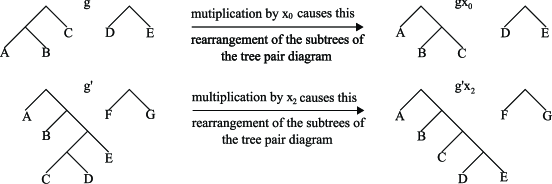
Figure 1. A depiction of the rearrangement of the subtrees of a tree pair diagram after multiplication by $x_{0}$ and $x_{2}$. Capital letters represent (possibly empty) subtrees of the original tree pair diagram. Multiplication by $x_{i}^{\pm 1}$ causes an analogous rearrangement of the subtrees at level $i+1$.

Our formula for the word length of elements $g\in F$ with respect to the generating set $X_{n}=\{x_{0},x_{1},\cdots,x_{n}\}$ has two components. The first we call $l_{\infty}(g)$, as it is the word length of $g$ with respect to the standard infinite generating set $\{x_{i}|i\geq 0\}$ for $F$. This quantity is simply the number of carets in the unique reduced tree pair diagram representing $g$ which are not right carets. The second component in the word length formula is twice what we term the penalty weight of the element. To make this precise, we begin by distinguishing a particular type of caret in a single tree.

Definition 2.1 ([HST], Definition 3.1).

Caret $p$ in a tree $T$ has type N if caret $p+1$ is an interior caret which lies in the right subtree of $p$.

We use this definition to describe certain carets in the tree pair diagram for $g\in F$ which we call penalty carets as they help determine the penalty contribution to the word length $l_{n}(g)$. Let $g\in F$ have a reduced tree pair diagram $(T_{-},T_{+})$ in which the carets are numbered in infix order. By caret $p$ in $(T_{-},T_{+})$ we mean the pair of carets numbered $p$ in each tree.

Definition 2.2 ([HST], Definition 3.2).

Caret $p$ in a tree pair diagram $(T_{-},T_{+})$ is a penalty caret if either

1. $p$ has type $N$ in either $T_{-}$ or $T_{+}$, or

2. $p$ is a right caret in both $T_{-}$ and $T_{+}$ and caret $p$ is not the final caret in the tree pair diagram.

To compute the penalty contribution to the word length for a given $g=(T_{-},T_{+})\in F$ we use the following procedure. Using a notion of caret adjacency defined below, we take the two trees $T_{-}$ and $T_{+}$ and construct a single tree ${\mathcal{P}}$, called a penalty tree, whose vertices correspond to a subset of the carets of $T_{-}$ and $T_{+}$, necessarily including the penalty carets. This tree is assigned a weight according to the arrangement of its vertices. Minimizing this weight over all possible penalty trees that can be constructed using the adjacencies between the carets of $T_{-}$ and $T_{+}$ yields the penalty weight $p_{n}(g)$. We may now state the word length formula precisely:

Theorem 2.1 ([HST], Theorem 3.3).

For every $g\in F$, the word length of $g$ with respect to the generating set $X_{n}=\{x_{0},x_{1},\cdots,x_{n}\}$ is given by the formula

$$l_{X_{n}}(g)=l_{n}(g)=l_{\infty}(g)+2p_{n}(g)$$

where $l_{\infty}(g)$ is the number of carets in the reduced tree pair diagram for $g$ which are not right carets, and $p_{n}(g)$ is the penalty weight of $g$.

Constructing penalty trees for elements $g\in F$ requires a concept of directed caret adjacency, which is an extension of the infix order. To define the concept of adjacency between carets in a single tree $T$, we view each caret as a space rather than an inverted v. The point of intersection of the left and right edges of the caret naturally splits the boundary of this space into a left and right component. The space is bounded on the right (resp. left) by a generalized right (resp. left) edge. The generalized right (resp. left) edge may consist of actual left (resp. right) edges of other carets in the tree, in addition to the actual right (resp. left) edge of the caret itself. Let $p$ and $q$ denote carets in a tree pair diagram $(T_{-},T_{+})$ and assume that $p<q$. We say that $p$ is adjacent to $q$, written $p\prec q$, if there is a caret edge, in either $T_{-}$ or $T_{+}$, which is both part of the generalized right edge of caret $p$ and the generalized left edge of caret $q$. We equivalently say that traversing the generalized left edge of caret $q$ takes you to caret $p$ in at least one tree. It is always true that carets $p$ and $p+1$ satisfy $p\prec p+1$. Although the ordering of carets given by infix number is not symmetric but is transitive, the notion of caret adjacency is neither symmetric nor transitive. Figure 2 shows an example of a single tree with the spaces corresponding to different carets shaded. In this tree, in addition to the adjacency relationships $p\prec p+1$ for $1\leq p\leq 10$, we also have $1\prec 3$, $5\prec 10$, $6\prec 10$, $6\prec 9$ and $7\prec 9$.

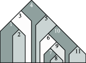
Figure 2. The shaded areas represent the carets of the tree, which are labeled in infix order.

We introduce a dummy caret denoted $v_{0}$ which is adjacent to all left carets in both $T_{-}$ and $T_{+}$. One can think of $v_{0}$ as being the space to the left of the left side of each tree. We now construct a penalty tree ${\mathcal{P}}$ corresponding to the pair of trees $(T_{-},T_{+})$, which has this dummy caret $v_{0}$ as its root, according to the following rules.

1. The vertices of ${\mathcal{P}}$ are a subset of the carets in the tree pair diagram, which we refer to by infix numbers: $0=v_{0},1,2,\cdots,k$, always including $v_{0}$.

2. A directed edge may be drawn from vertex $p$ to vertex $q$ in ${\mathcal{P}}$ if $p\prec q$.

3. There is a vertex for every penalty caret in $(T_{-},T_{+})$.

4. Each leaf of ${\mathcal{P}}$ corresponds to a penalty caret of $(T_{-},T_{+})$. The only exception to this is when ${\mathcal{P}}$ consists only of the root $v_{0}$ and no edges.

The penalty tree ${\mathcal{P}}$ is oriented in the sense that there is a unique path from $v_{0}$ to every vertex $p\in{\mathcal{P}}$, and if this path passes through vertices $v_{0},p_{1},p_{2},\ldots,p_{i}=p$ then we must have $v_{0}\prec p_{1}\prec\cdots\prec p_{i}=p$. Two vertices $p,q$ in the tree are comparable if there is either a path $p=w_{1},w_{2},\ldots,w_{i+1}=q$ or $q=w_{1},w_{2},\ldots,w_{i+1}=p$ with $w_{j}\prec w_{j+1},\forall j=1,\ldots,i+1$, and in this case we say $d_{{\mathcal{P}}}(p,q)=i$.

The penalty weight of a penalty tree is bounded above by the number of vertices on the tree, but not all vertices on the tree contribute to the weight. More precisely, we define:

Definition 2.3 ([HST], Definition 3.4).

The n-penalty weight $p_{n}({\mathcal{P}})$ of a penalty tree ${\mathcal{P}}$ associated to $g=(T_{-},T_{+})\in F$ is the number of vertices $v_{i}\in{\mathcal{P}}$ such that $d_{{\mathcal{P}}}(v_{0},v_{i})\geq 2$ and there exists a leaf $l_{i}$ in ${\mathcal{P}}$ with $d_{{\mathcal{P}}}(v_{i},l_{i})\geq n-1$. These vertices are called the weighted carets.

To compute the penalty contribution $p_{n}(g)$ to the word length $l_{n}(g)$ for $g\in F$, we must minimize the penalty weight over all penalty trees associated to $g$.

Definition 2.4 ([HST],Definition 3.5).

For an element $g\in F$, define the penalty weight of the element $G\in F$, denoted $p_{n}(g)$ by

$$p_{n}(g)=min\{p_{n}({\mathcal{P}})|{\mathcal{P}}\mbox{ is a penalty tree for }g=(T_{-},T_{+})\}$$

We have now defined both components of the word length formula given in Theorem 2.1.

3. Coarse isometries and convexity

Recall that a map $f$ between two metric spaces $G$ and $H$ is a quasi-isometry if there are positive constants K and C so that for every pair of points $g_{1},g_{2}\in G$,

$$\frac{1}{K}d_{G}(g_{1},g_{2})-C\leq d_{H}(f(g_{1}),f(g_{2}))\leq Kd_{G}(g_{1},g_{2})+C.$$

If the constant $K$ can be chosen to be $1$, we call $f$ a C-coarse isometry. Given a group $G$ and a finite generating set $X$, G can be regarded as a metric space using the wordlength metric, namely, $d_{X}(g,h)=min\{n|gh^{-1}=\alpha_{1}\alpha_{2}\cdots\alpha_{n},\alpha_{i}^{\pm 1}\in X\}$. We denote $G$, viewed as a metric space in this way, by $(G,X)$. Equivalently, one can view the Cayley graph $\Gamma(G,X)$ as a metric space by declaring each edge to have length 1. Recall that for any finitely generated group $G$ with finite generating sets $X$ and $Y$, the identity map between $(G,X)$ as $(G,Y)$ is a quasi-isometry. In general, it is unknown to what extent quasi-isometries preserve convexity properties, but in the special case of a coarse-isometry, we obtain the following:

Theorem 3.1.

Let $f:(G,X_{G})\rightarrow(H,X_{H})$ be a $C$-coarse-isometry. If $(G,X_{G})$ is not minimally almost convex, then $(H,X_{H})$ is not almost convex.

Proof.

Let $g$ be any coarse inverse for $f$, which is easily seen to be a coarse isometry as well. Without loss of generality, we may assume that $g$ is also a $C$-coarse isometry.

Suppose that $(H,X_{H})$ is almost convex. Then for each $n\geq 2$, there is an almost convexity constant $K(n)$. Fix $M>2C+1$, and let $K=K(2M+C)$. Let $n>K+M+C$.

Since $(G,X_{G})$ is not minimally almost convex, we can find $x,y\in B(n)\subset\Gamma(G,X_{G})$ with $d_{G}(x,y)=2$ so that the shortest path from $x$ to $y$ which remains in $B(n)$ has length $2n$. Since we can always construct a path of this length passing through the identity, let $\gamma$ be such a path containing the identity.

Consider the closed loop $\eta$ obtained by concatenating $\gamma$ with the path of length two between $x$ and $y$. Let $z$ denote the point in $B(n+1)$ at distance one from $x$ and $y$. Choose $a$ and $b$ on $\gamma$, with $a$ on the subpath of $\gamma$ from $x$ to the identity, and $b$ between $y$ and the identity, so that $d_{G}(a,Id)=d_{G}(b,Id)$ and $d_{G}(a,z)=d_{G}(b,z)=M$. Let $\eta_{1}$ be the subpath of $\gamma$ containing $a,\ b$ and the identity, and $\eta_{2}$ is the remaining subpath of $\eta$.

Consider $f(a)$ and $f(b)$, elements of the Cayley graph $\Gamma(H,X_{H})$. We know that $d_{H}(f(a),f(b))\leq 2M+C$. Since we are assuming that $(H,X_{H})$ is almost convex, there must be a path $\xi$ from $f(a)$ to $f(b)$ whose length is at most $K$, and which remains in the ball $B(D)$, where $D$ is defined by $D=\max\{d_{H}(f(a),id),\ d_{H}(f(b),id)\}\leq d_{G}(a,id)+C$.

Consider the image of $\xi$ under $g$, the coarse inverse to $f$. Since $length(\eta_{1})=2n-2M+2>2(K+C+M)-2M+2>2K+2C$ and $length(g(\xi))\leq K+C$, we see that $length(g(\xi))<length(\eta_{1})$. We now show that this path stays in $B(n)$, contradicting the fact that any path from $x$ to $y$ in $B(n)$ has length $2n$.

The maximum distance of any point on $\xi$ from the identity in $H$ is $D$. Thus the maximum distance of any point on $g(\xi)$ from the identity of $G$ is $D+C\leq d_{G}(a,id)+2C=n-M+1+2C$. Since $M>2C+1$, it follows that $g(\xi)\subset B_{G}(n)$.

By concatenating the portion of $\eta_{2}$ from $x$ to $a$, $g(\xi)$, and the portion of $\eta_{2}$ from $b$ to $y$, we obtain a path from $x$ to $y$ which remains inside of $B(n)$ and has length less than $2n$, a contradiction since $(G,X_{G})$ is not minimally almost convex. ∎

3.1. Application to Thompson’s group $F$

In [CT1] it is shown that Thompson’s group $F$ is not almost convex with respect to the standard finite generating set $\{x_{0},x_{1}\}$. A natural question is whether $F$ is not almost convex with respect to any finite generating set. We use Theorem 3.1 to extend this result to finite generating sets for $F$ of the form $\{x_{0},x_{n}\}$.

Belk and Bux in [BBu] show that Thompson’s group $F$ is not minimally almost convex with respect to the generating set $\{x_{0},x_{1}\}$. It is easy to see that the the word metrics in $(F,\{x_{0},x_{1}\})$ and$(F,\{x_{0},x_{n}\})$ differ by the additive constant $2(n-1)$, and thus the quasi-isometry between these two presentations for $F$ is a coarse isometry.

Combining these results with Theorem 3.1, we obtain the following corollary, which is a special case of Theorem 4.4 below.

Corollary 3.2.

Thompson’s group $F$ is not almost convex with respect to any generating set of the form $\{x_{0},x_{n}\}$.

4. Convexity results

The main goal of this section is to show that $F$ is not almost convex with respect to any generating set which is a subset of the standard infinite generating set; we note that in order for a subset of the standard infinite generating set to generate $F$, it must contain $x_{0}$. We extend the result of [BBu] which proves that $(F,\{x_{0},x_{1}\})$ is not minimally almost convex first to consecutive generating sets for $F$, and then to generating sets which contain $x_{0}$ and $x_{1}$ and are subsets of the standard infinite generating set. To obtain our ultimate result, that $F$ is not almost convex with respect to any generating set which is a subset of the infinite generating set for $F$ and contains $x_{0}$, we again discuss coarse isometries between different presentations for $F$.

We begin with the following:

Theorem 4.1.

Let $X_{n}=\{x_{0},x_{1},\cdots,x_{n}\}$ be a consecutive generating set for $F$ with $n\geq 2$. Then $F$ is not minimally almost convex with respect to $X_{n}$.

Proof.

We prove this by providing, for any $k>0$, a pair of group elements $g=g_{k}$ and $h=h_{k}$ satisfying $l_{n}(g)=l_{n}(h)=2k+2$ and $l_{n}(h^{-1}g)=2$, for which any path $\gamma$ from $g$ to $h$ that lies entirely within the ball of radius $2k+2$ must have length at least $4k+4$.

Let $g=g_{n}=x_{1}^{k+1}x_{k+n+1}x_{0}^{-k}=x_{n}x_{1}^{k+1}x_{0}^{-k}$ and $h=h_{n}=gx_{0}^{-1}x_{n}^{-1}=x_{1}^{k+1}x_{0}^{-(k+1)}$. The tree pair diagrams for these elements are given in Figure 3. In the tree pair diagrams for $g$ and $h$, we observe that $l_{\infty}(g)=l_{\infty}(h)=2k+2$. From Theorem 2.1 we see that $l_{n}(a)\geq l_{\infty}(a)$ for all $a\in F$, and since we have provided words above of length $2k+2$ for both $g$ and $h$, it follows that $l_{n}(g)=l_{n}(h)=2k+2$.

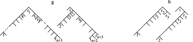
Figure 3. The tree pair diagrams representing the elements $g$ and $h$ used in the proof of Theorem 4.1.

Suppose there is a path $\gamma$ from $g$ to $h$ which lies within the ball of radius $2k+2$. We note that the only generator $x\in X_{n}$ so that the word length of $gx$ is less than the word length of $g$ is $x=x_{0}$. Thus the first vertex along $\gamma$ after $g$ is $gx_{0}$. In the negative tree for the tree pair representing $gx_{0}$, the caret $r_{n+2}$ is a right caret at level $n+3$, whereas in the tree pair diagram for $g$ it is a right caret at level $n+2$. Our argument relies on noting the level of this caret at successive vertices along the path $\gamma$.

In order for the path $\gamma$ to terminate at $h$, there is a point at which the pair of carets numbered $r_{n+2}$ in each tree must be removed as part of a reduction along $\gamma$. This requires caret $r_{n+2}$ from $T_{-}$ to be an interior caret at the point of reduction. Given the effect of multiplication by each generator on the tree pair diagram as described in Section 2, we observe that the generators in $X_{n}$ cannot move any right caret off the right side of the tree unless it is at level 1 through $n+1$. Hence, we conclude that there is a smallest nontrivial prefix $\gamma_{0}$ of $\gamma$ so that in $g\gamma_{0}=f$ the caret $r_{n+2}$ in the negative tree for $f$ is a right caret at level $n+1$.

Let $(S_{-},S_{+})$ be the tree pair diagram for $f=g\gamma_{0}$ which is constructed from the tree pair diagram $(T_{-},T_{+})$ for $g$ by altering these trees according to multiplication by each generator of $\gamma_{0}$, but without performing any possible reductions. During this process, the carets in $T_{+}$ remain unchanged, though additional carets may be added to $T_{+}$ to form $S_{+}$. Hence, $S_{+}$ contains $T_{+}$ as a subtree, and the tree pair diagram $(S_{-},S_{+})$ may be unreduced.

We first show that the tree pair diagram $(S_{-},S_{+})$ constructed in this way must be unreduced, and that when the reduction is accomplished, some of the original carets from $T_{+}$ will be removed from $S_{+}$. If this was not the case, then in $S_{-}$ there would be at least $k+1$ carets with smaller infix numbers than $r_{n+1}$ which were not right carets, and thus counted towards $l_{\infty}(f)$. Additionally, in $S_{+}$ there would also be $k+1$ interior carets with infix numbers less than $r_{n+2}$, and caret $r_{n+2}$ itself is also an interior caret. This implies that $l_{\infty}(f)\geq 2k+3$, contradicting the fact that $f\in B(2k+2)$. Thus there must be some reduction of the carets of $T_{+}$, viewed as a subtree of $S_{+}$, in order to obtain the reduced tree pair diagram for $g\gamma_{0}=f$.

We now consider which carets of $T_{+}$, viewed as a subtree of $S_{+}$ might be reduced; in order for a caret to be reduced after multiplication by a particular generator, it must be exposed, that is, both leaves have valence one. The only exposed carets of $T_{+}$ itself are carets $2$ and $r_{n+2}$. Since caret $r_{n+2}$ is a right caret in $S_{-}$, and not the final right caret, it is not exposed in $S_{-}$. Therefore, it must be that in reducing $(S_{-},S_{+})$, the original caret $2$ from the infix ordering on $T_{+}$ must cancel. We claim that in $S_{-}$, caret $2$ must be a child of caret $1$. If, in forming $S_{+}$, no carets were added to either leaf of caret $2$, then caret $2$ is exposed in $S_{+}$, and hence it is exposed in $S_{-}$, which implies that caret $2$ is a child of caret $1$ in $S_{-}$. If, on the other hand, carets were added to the leaves of caret $2$ in forming $S_{+}$, then they must all cancel in $(S_{-},S_{+})$ before caret $2$ does. But this means that in $S_{-}$, these added carets must also hang from the leaves of caret $2$, and once again, caret $2$ is a child of caret $1$ in $S_{-}$.

The fact that caret $2$ is a child of caret $1$ in $S_{-}$ provides a lower bound on $l_{n}(h^{-1}f)$ as follows. To form the tree pair diagram for $h^{-1}f$, consider the unreduced tree pair diagram $(S_{-},S_{+})$. If $h=(H_{-},H_{+})$, to form this product we consider these trees in the order $S_{-}\ S_{+}\ H_{+}\ H_{-}$, and add carets to each pair to ensure that the middle trees are identical. Thus we must at least add the string of right carets $r_{4},\ldots,r_{n+1},r_{n+3}$, with caret $r_{n+2}$ the left child of $r_{n+3}$, from $S_{+}$ to both trees in the diagram $(H_{+},H_{-})$ in order to perform this multiplication. Since in $S_{-}$, caret $2$ is a child of caret $1$, but in $H_{-}$ caret $1$ is a child of caret $2$, caret $1$ cannot reduce in the product $h^{-1}f$. Hence, because of their configuration in $H_{-}$, the entire string of carets $1,2,\cdots,k,r_{1}$ do not reduce in the product $h^{-1}f$. Also, as we remarked above, caret $r_{n+2}$ is not removed through reduction in this product. Hence we obtain the following lower bound on the word length of $h^{-1}f$: $l_{n}(h^{-1}f)\geq l_{\infty}(h^{-1}f)\geq 2(k+1)+1=2k+3.$

Let $\gamma_{1}$ be the subpath of $\gamma$ from $f=g\gamma_{0}$ to $h$. Since $l_{n}(h^{-1}f)\geq 2k+3$, it follows that $|\gamma_{1}|\geq 2k+3$. But traversing $\gamma_{0}$ in reverse, followed by $x_{0}^{-1}$ and then $x_{n}^{-1}$ yields another path from $f$ to $h$, so similarly $|\gamma_{0}|+2\geq 2k+3$, and hence $|\gamma_{0}|\geq 2k+1$. This implies that $|\gamma|=|\gamma_{0}|+|\gamma_{1}|\geq 4k+4$. ∎

In the proof above, both $g$ and $h$ are be represented by words of length $2k+2$ involving only the generators $x_{0}^{\pm 1},x_{1}^{\pm 1}$, and $x_{n}^{\pm 1}$, namely, $g=x_{n}x_{1}^{k+1}x_{0}^{-k}$ and $h=x_{1}^{k+1}x_{0}^{-(k+1)}$. Hence, the above result can be extended to any generating set for $F$ which is a finite subset of the standard infinite generating set containing $x_{0}$ and $x_{1}$.

Theorem 4.2.

Let $X=\{x_{0},x_{1},x_{i_{1}},x_{i_{2}},\cdots,x_{i_{j}}\}$, where $1<i_{1}<\cdots<i_{j}$, be a generating set for $F$. Then $F$ is not minimally almost convex with respect to $X$.

Proof.

The identity map on $G$ is a quasi-isometry between the metric spaces $(G,X)$ and $(G,X_{i_{j}})$, where $X_{i_{j}}=\{x_{0},x_{1},x_{2},x_{3}\cdots,x_{i_{j}}\}$. Since $X\subset X_{i_{j}}$, we remark that $d_{X_{i_{j}}}(a,b)\leq d_{X}(a,b)$ for any $a,b\in F$. In particular, $d_{X_{i_{j}}}(a,Id))\leq d_{X}(a,Id)$ for any $a\in F$.

Assume that $(F,X)$ is minimally almost convex. It is proven in Theorem 4.1 that $(F,X_{i_{j}})$ is not minimally almost convex. Let $h=h_{k}=x_{1}^{k+1}x_{0}^{-(k+1)}$ and $g=g_{k}=x_{1}^{k+1}x_{k+i_{j}+1}x_{0}^{-k}$ be the group elements used in the proof of Theorem 4.1. It is clear that $2k+2=d_{X_{i_{j}}}(h,id)=d_{X}(h,id)$ and $2k+2=d_{X_{i_{j}}}(g,id)=d_{X}(g,id)$; if there was a shorter expression for either $g$ or $h$ with respect to $X$, then there would be one with respect to $X_{i_{j}}$ as well. In addition, it is clear that since $g^{-1}h=x_{i_{j}+1}^{-1}x_{0}^{-1}=x_{0}^{-1}x_{i_{j}}^{-1}$, we have $d_{X_{i_{j}}}(g,h)=d_{X}(g,h)=2$.

Since $(F,X)$ is assumed to be minimally almost convex, there is a path $\gamma$ of length at most $4k+3$ connecting $g$ and $h$ which lies within the ball of radius $2k+2$ relative to $X$. Since each group element $a$ along this path satisfies $d_{X_{i_{j}}}(a,id))\leq d_{X}(a,id)\leq 2k+2$, this contradicts the assumption that $(F,X_{i_{j}})$ is not minimally almost convex. Thus we conclude that $(F,X)$ cannot be minimally almost convex. ∎

To extend the result of Theorem 6.1 of [HST] to arbitrary finite subsets of the infinite generating set containing $x_{0}$, we show first that word length with respect to one of these arbitrary generating sets differs from word length with respect to some generating set containing $x_{1}$ only by an additive constant.

Lemma 4.3.

Let $X=\{x_{0},x_{i_{1}},x_{i_{2}},\cdots,x_{i_{j}}\}$ be a generating set for $F$, and form a new generating set $Y=\{x_{0},x_{1},x_{i_{2}-i_{1}+1},x_{i_{3}-i_{1}+1},\ldots x_{i_{j}-i_{1}+1}\}$. Then $(F,X)$ and $(F,Y)$ are coarsely isometric.

Proof.

Let $g\in F$, and suppose $g=\alpha_{1}\alpha_{2}\cdots\alpha_{m}$, where $\alpha_{k}^{\pm 1}\in Y$. Then

$$g=x_{0}^{i_{1}-1}\left(x_{0}^{1-i_{1}}gx_{0}^{i_{1}-1}\right)x_{0}^{1-i+1}=x_{0}^{i_{1}-1}\bar{\alpha_{1}}\bar{\alpha_{2}}\cdots\bar{\alpha_{m}}x_{0}^{i_{1}-1},$$

where $\bar{\alpha_{k}}=x_{0}^{1-i_{1}}\alpha_{k}x_{0}^{i_{1}-1}$. Now in the cases where $\alpha_{k}=x_{0}^{\pm 1}$, we have $\bar{\alpha_{k}}=\alpha_{k}$, and in the cases where $\alpha_{k}=x_{l}^{\pm 1}$ with $l\geq 1$, then $\bar{\alpha_{k}}=x_{l+i_{1}-1}^{\pm 1}\in X$. Hence $l_{X}(g)\leq l_{Y}(g)+2(i_{1}-1)$. Similarly, one sees that $l_{Y}(g)\leq l_{X}(g)+2(i_{1}-1)$. Hence, $l_{X}(g)-2(i_{1}-1)\leq l_{Y}(g)\leq l_{X}(g)+2(i_{1}-1)$ and $l_{Y}(g)-2(i_{1}-1)\leq l_{X}(g)\leq l_{Y}(g)+2(i_{1}-1)$. ∎

Finally, we apply Theorem 3.1 to $F$ with the two generating sets $X$ and $Y$ of the preceding theorem to obtain:

Theorem 4.4.

Let $X$ be any subset of the standard infinite generating set for $F$ which includes $x_{0}$. Then $F$ is not almost convex with respect to $X$.

References

- [BBr] J.M. Belk and K.S. Brown, Forest diagrams for Thompson’s group , Int. J. Algebra Comput.15(2005), no. 5-6, 815-850.
- [BBu] J.M. Belk and K. Bux, Thompson’s Group F is minimally nonconvex, in Geometric methods in group theory, Contemp. Math., 372, Amer. Math. Soc. (2005), 131-146.
- [C] J. Cannon, Almost convex groups, Geom. Dedicata 22(1987), 197-210.
- [CFGT] J. Cannon, W. Floyd, M. Grayson, and W. Thurston, Solvgroups are not almost convex, Geom. Dedicata 31(1989), 291-300.
- [CFP] J.W. Cannon, W.J. Floyd, and W.R. Parry, Introductory notes on Richard Thompson’s groups, Enseign. Math. 42(1996), 215-256.
- [CT1] S. Cleary and J. Taback, Thompson’s group is not almost convex, J. Algebra 270(2003), no.1., 133-149.
- [CT2] S. Cleary and J. Taback, Combinatorial Properties of Thompson’s group , Trans. Amer. Math. Soc. 356 (2004), no. 7., 2825-2849 (electronic).
- [EH] M. Elder and S. Hermiller, Minimal almost convexity, Journal of Group Theory 8 (2005), no. 2., 239–266.
- [F] S.B. Fordham, Minimal length elements of Thompson’s group , Geom. Dedicata, 99(2003), 179-220.
- [G] V.S. Guba, On the Properties of the Cayley Graph of Richard Thompson’s Group , in International Conference on Semigroups and Groups in honor of the 65th birthday of Prof. John Rhodes. Internat. J. Algebra Comput. 14(2004), no. 5-6, 677-702.
- [HST] M. Horak, M.Stein, and J. Taback, Computing word length in alternate presentations of Thompson’s group , preprint.
- [K] I. Kapovich, A note on the Poéenaru condition, J. Group Theory, 5(2002), pp. 119-127.
- [MS] C.F. Miller, III and M. Shapiro, Solvable Baumslag-Solitar groups are not almost convex, Geom. Dedicata 72(1998), no. 2, 123-127.
- [SS] M. Shapiro and M. Stein, Almost Convex Groups and the Eight Geometries, Geom. Dedicata 55 (1995), 125-140.
- [T] C. Thiel Zur Fast-Konvexitt einiger nilpotenter Gruppen, Bonner Math. Schriften (1992).