Lectures on Random Matrix Models. The Riemann-Hilbert Approach

Abstract.

This is a review of the Riemann-Hilbert approach to the large $N$ asymptotics in random matrix models and its applications. We discuss the following topics: random matrix models and orthogonal polynomials, the Riemann-Hilbert approach to the large $N$ asymptotics of orthogonal polynomials and its applications to the problem of universality in random matrix models, the double scaling limits, the large $N$ asymptotics of the partition function, and random matrix models with external source.

1. Introduction

This article is a review of the Riemann-Hilbert approach to random matrix models. It is based on a series of 5 lectures given by the author at the miniprogram on “Random Matrices and their Applications” at the Centre de recherches math ematiques, Université de Montreal, in June 2005. The review contains 5 lectures:

1. Lecture 1. Random matrix models and orthogonal polynomials.

2. Lecture 2. Large $N$ asymptotics of orthogonal polynomials. The Riemann-Hilbert approach.

3. Lecture 3. Double scaling limit in a random matrix model.

4. Lecture 4. Large $N$ asymptotics of the partition function of random matrix models.

5. Lecture 5. Random matrix models with external source.

The author would like to thank John Harnad for his invitation to give the series of lectures at the miniprogram. The lectures are based on the joint works of the author with several coauthors: Alexander Its, Arno Kuijlaars, Alexander Aptekarev, and Bertrand Eynard. The author is grateful to his coauthors for an enjoyable collaboration.

Lecture 1. Random matrix models and orthogonal polynomials

The first lecture gives an introduction to random matrix models and their relations to orthogonal polynomials.

2. Unitary ensembles of random matrices

2.1. Unitary ensemble with polynomial interaction

Let $M=\left(M_{jk}\right)_{j,k=1}^{N}$ be a random Hermitian matrix, $M_{kj}=\overline{M_{jk}}$, with respect to the probability distribution

$$d\mu_{N}(M)=\frac{1}{Z_{N}}\,e^{-N{{\operatorname{Tr}\,}}V(M)}dM,$$ (2.1)

where

$$V(M)=\sum_{i=1}^{p}t_{j}M^{j},\qquad p=2p_{0},\qquad t_{p}>0,$$ (2.2)

is a polynomial,

$$dM=\prod_{j=1}^{N}dM_{jj}\prod_{j\not=k}^{N}d{\operatorname{Re\,}}M_{jk}d{\operatorname{Im\,}}M_{jk},$$ (2.3)

the Lebesgue measure, and

$$Z_{N}=\int_{\mathcal{H}_{N}}e^{-N{{\operatorname{Tr}\,}}V(M)}dM,$$ (2.4)

the partition function. The distribution $\mu_{N}(dM)$ is invariant with respect to any unitary conjugation,

$$M\to U^{-1}MU,\quad U\in U(N),$$ (2.5)

hence the name of the ensemble.

2.2. Gaussian unitary ensemble

For $V(M)=M^{2}$, the measure $\mu_{N}$ is the probability distribution of the Gaussian unitary ensemble (GUE). In this case,

$${{\operatorname{Tr}\,}}V(M)={{\operatorname{Tr}\,}}M^{2}=\sum_{j,k=1}^{N}M_{kj}M_{jk}=\sum_{j=1}^{N}M_{jj}^{2}+2\sum_{j>k}|M_{jk}|^{2},$$ (2.6)

hence

$$\mu_{N}^{\rm GUE}(dM)=\frac{1}{Z_{N}^{\rm GUE}}\,\prod_{j=1}^{N}\left(e^{-NM_{jj}^{2}}\right)\prod_{j>k}\left(e^{-2N|M_{jk}|^{2}}\right)dM,$$ (2.7)

so that the matrix elements in GUE are independent Gaussian random variables. The partition function of GUE is evaluated as

$$Z_{N}^{\rm GUE} =\int_{\mathcal{H}_{N}}\prod_{j=1}^{N}\left(e^{-NM_{jj}^{2}}\right)\prod_{j>k}\left(e^{-2N|M_{jk}|^{2}}\right)dM=\left(\frac{\pi}{N}\right)^{N/2}\left(\frac{\pi}{2N}\right)^{N(N-1)/2}$$ (2.8)

$$=\left(\frac{\pi}{N}\right)^{N^{2}/2}\left(\frac{1}{2}\right)^{N(N-1)/2}.$$

If $V(M)$ is not quadratic then the matrix elements $M_{jk}$ are dependent.

2.3.  Topological large $N$ expansion

Consider the free energy of the unitary ensemble of random matrices,

$$F_{N}^{0}=-N^{-2}\ln Z_{N}=-N^{-2}\int_{\mathcal{H}_{N}}e^{-N{{\operatorname{Tr}\,}}V(M)}dM,$$ (2.9)

and the normalized free energy,

$$F_{N}=-N^{-2}\ln\frac{Z_{N}}{Z_{N}^{\rm GUE}}=-N^{-2}\ln\frac{\int_{\mathcal{H}_{N}}e^{-N{{\operatorname{Tr}\,}}V(M)}dM}{\int_{\mathcal{H}_{N}}e^{-N{{\operatorname{Tr}\,}}M^{2}}dM}.$$ (2.10)

The normalized free energy can be expessed as

$$F_{N}=-N^{-2}\ln\left\langle e^{-N{{\operatorname{Tr}\,}}V_{1}(M)}\right\rangle$$ (2.11)

where $V_{1}(M)=V(M)-M^{2}$ and

$$\left\langle f(M)\right\rangle=\frac{\int_{\mathcal{H}_{N}}f(M)e^{-N{{\operatorname{Tr}\,}}M^{2}}dM}{\int_{\mathcal{H}_{N}}e^{-N{{\operatorname{Tr}\,}}M^{2}}dM},$$ (2.12)

the mathematical expectation of $f(M)$ with respect to GUE. Suppose that

$$V(M)=M^{2}+t_{3}M^{3}+\ldots+t_{p}M^{p}.$$ (2.13)

Then (2.10) reduces to

$$F_{N}=-N^{-2}\ln\left\langle e^{-N{{\operatorname{Tr}\,}}(t_{3}M^{3}+\ldots+t_{p}M^{p})}\right\rangle.$$ (2.14)

$F_{N}$ can be expanded into the asymptotic series in negative powers of $N^{2}$,

$$F_{N}\sim F+\sum_{g=1}^{\infty}\frac{F^{(2g)}}{N^{2g}},$$ (2.15)

which is called the topological large $N$ expansion. The Feynman diagrams representing $F^{(2g)}$ are realized on a two-dimensional Riemann closed manifold of genus $g$, and, therefore, $F_{N}$ serves as a generating function for enumeration of graphs on Riemannian manifolds, see, e.g., the works [BIZ], [BIPZ], [IZ], [DiF], [EM], [EMP]. This in turn leads to a fascinating relation between the matrix integrals and the quantum gravity, see, e.g., the works [DGZ], [Wit], and others.

2.4. Ensemble of eigenvalues

The Weyl integral formula implies, see, e.g., [Meh], that the distribution of eigenvalues of $M$ with respect to the ensemble $\mu_{N}$ is given as

$$d\mu_{N}(\lambda)=\frac{1}{\tilde{Z}_{N}}\,\prod_{j>k}(\lambda_{j}-\lambda_{k})^{2}\prod_{j=1}^{N}e^{-NV(\lambda_{j})}d\lambda,$$ (2.16)

where

$$\tilde{Z}_{N}=\int\prod_{j>k}(\lambda_{j}-\lambda_{k})^{2}\prod_{j=1}^{N}e^{-NV(\lambda_{j})}d\lambda,\qquad d\lambda=d\lambda_{1}\ldots d\lambda_{N}.$$ (2.17)

Respectively, for GUE,

$$d\mu_{N}^{\rm GUE}(\lambda)=\frac{1}{\tilde{Z}_{N}^{\rm GUE}}\,\prod_{j>k}(\lambda_{j}-\lambda_{k})^{2}\prod_{j=1}^{N}e^{-N\lambda_{j}^{2}}d\lambda,$$ (2.18)

where

$$\tilde{Z}_{N}^{\rm GUE}=\int\prod_{j>k}(\lambda_{j}-\lambda_{k})^{2}\prod_{j=1}^{N}e^{-N\lambda_{j}^{2}}d\lambda.$$ (2.19)

The constant $\tilde{Z}_{N}^{\rm GUE}$ is a Selberg integral, and its exact value is

$$\tilde{Z}_{N}^{\rm GUE}=\frac{(2\pi)^{N/2}}{(2N)^{N^{2}/2}}\prod_{n=1}^{N}n!$$ (2.20)

see, e.g., [Meh]. The partition functions $Z_{N}$ and $\tilde{Z}_{N}$ are related as follows:

$$\frac{\tilde{Z}_{N}}{Z_{N}}=\frac{\tilde{Z}_{N}^{\rm GUE}}{Z_{N}^{\rm GUE}}=\frac{1}{\pi^{N(N-1)/2}}\prod_{n=1}^{N}n!$$ (2.21)

One of the main problems is to evaluate the large $N$ asymptotics of the partition function $\tilde{Z}_{N}$ and of the correlations between eigenvalues.

The $m$-point correlation function is given as

$$R_{mN}(x_{1},\dots,x_{m})=\frac{N!}{(N-m)!}\int_{{\mathbb{R}}^{N-m}}p_{N}(x_{1},\dots,x_{N})dx_{m+1}\dots dx_{N},$$ (2.22)

where

$$p_{N}(x_{1},\dots,x_{N})=\widetilde{Z}_{N}^{-1}\prod_{j>k}(x_{j}-x_{k})^{2}\prod_{j=1}^{N}e^{-NV(x_{j})}.$$ (2.23)

The Dyson determinantal formula for correlation functions, see, e.g., [Meh], is

$$R_{mN}(x_{1},\dots,x_{m})=\det\left(K_{N}(x_{k},x_{l})\right)_{k,l=1}^{m},$$ (2.24)

where

$$K_{N}(x,y)=\sum_{n=0}^{N-1}\psi_{n}(x)\psi_{n}(y)$$ (2.25)

and

$$\psi_{n}(x)=\frac{1}{h_{n}^{1/2}}P_{n}(x)e^{-NV(x)/2},$$ (2.26)

where $P_{n}(x)=x^{n}+a_{n-1}x^{n-1}+\dots$ are monic orthogonal polynomials,

$$\int_{-\infty}^{\infty}P_{n}(x)P_{m}(x)e^{-NV(x)}dx=h_{n}\delta_{nm}.$$ (2.27)

Observe that the functions $\psi_{n}(x)$, $n=0,1,2,\ldots$, form an orthonormal basis in $L^{2}({\mathbb{R}}^{1})$, and $K_{N}$ is the kernel of the projection operator on tne $N$ dimensional space generated by the first $N$ functions $\psi_{n}$, $n=0,\ldots,N-1$. The kernel $K_{N}$ can be expressed in terms of $\psi_{N-1}$, $\psi_{N}$ only, due to the Christoffel-Darboux formula. Consider first recurrent and differential equations for the functions $\psi_{n}$.

2.5. Recurrence equations and discrete string equations for orthogonal polynomials

The orthogonal polynomials satisfy the three term recurrent relation, see, e.g. [Sze],

$$xP_{n}(x) =P_{n+1}(x)+\beta_{n}P_{n}(x)+\gamma_{n}^{2}P_{n-1}(x),$$ (2.28)

$$\gamma_{n} =\left(\frac{h_{n}}{h_{n-1}}\right)^{1/2}>0\,,\quad n\geq 1;\qquad\gamma_{0}=0.$$

For the functions $\psi_{n}$ it reads as

$$x\psi_{n}(x)=\gamma_{n+1}\psi_{n+1}(x)+\beta_{n}\psi_{n}(x)+\gamma_{n}\psi_{n-1}(x).$$ (2.29)

This allows the following calculation:

$$(x-y)\sum_{n=0}^{N-1}\psi_{n}(x)\psi_{n}(y) =\sum_{n=0}^{N-1}\left[\left(\gamma_{n+1}\psi_{n+1}(x)+\beta_{n}\psi_{n}(x)+\gamma_{n}\psi_{n-1}(x)\right)\psi_{n}(y)\right.$$ (2.30)

$$\left.-\psi_{n}(x)\left(\gamma_{n+1}\psi_{n+1}(y)+\beta_{n}\psi_{n}(y)+\gamma_{n}\psi_{n-1}(y)\right)\right]$$

$$=\gamma_{N}\left[\psi_{N}(x)\psi_{N-1}(y)-\psi_{N-1}(x)\psi_{N}(y)\right]$$

(telescopic sum), hence

$$K_{N}(x,y)=\sum_{n=0}^{N-1}\psi_{n}(x)\psi_{n}(y)=\gamma_{N}\frac{\psi_{N}(x)\psi_{N-1}(y)-\psi_{N-1}(x)\psi_{N}(y)}{x-y}\,.$$ (2.31)

which is the Christoffel-Darboux formula. For the density function we obtain that

$$p_{N}(x)=\frac{Q_{N}(x,x)}{N}=\frac{\gamma_{N}}{N}\left[\psi^{\prime}_{N}(x)\psi_{N-1}(x)-\psi^{\prime}_{N-1}(x)\psi_{N}(x)\right]\,.$$ (2.32)

Consider a matrix $Q$ of the operator of multiplication by $x$, $f(x)\to xf(x)$, in the basis $\{\psi_{n}(x)\}$. Then by (2.29), $Q$ is the symmetric tridiagonal Jacobi matrix,

$$Q=\begin{pmatrix}\beta_{0}&\gamma_{1}&0&0&\dots\\ \gamma_{1}&\beta_{1}&\gamma_{2}&0&\dots\\ 0&\gamma_{2}&\beta_{2}&\gamma_{3}&\dots\\ 0&0&\gamma_{3}&\beta_{3}&\dots\\ \vdots&\vdots&\vdots&\vdots&\ddots\end{pmatrix}.$$ (2.33)

Let $P=\left(P_{nm}\right)_{n,m=0,1,2,\dots}$ be a matrix of the operator $f(z)\to f^{\prime}(z)$ in the basis $\psi_{n}(z)$, $n=0,1,2,\dots$, so that

$$P_{nm}=\int_{-\infty}^{\infty}\psi_{n}(x)\psi^{\prime}_{m}(x)\,dx.$$ (2.34)

Then $P_{mn}=-P_{nm}$ and

$$\psi_{n}^{\prime}(z) =-\frac{NV^{\prime}(z)}{2}\psi_{n}(z)+\frac{P^{\prime}_{n}(z)}{\sqrt{h_{n}}}e^{-NV(z)/2}=-\frac{NV^{\prime}(z)}{2}\psi_{n}(z)+\frac{n}{\gamma_{n}}\psi_{n-1}(z)+\dots,$$ (2.35)

hence

$$\left[P+\frac{NV^{\prime}(Q)}{2}\right]_{nn}=0,\qquad\left[P+\frac{NV^{\prime}(Q)}{2}\right]_{n,n+1}=0,$$ (2.36)

$$\left[P+\frac{NV^{\prime}(Q)}{2}\right]_{n,n-1}=\frac{n}{\gamma_{n}}\,.$$

Since $P_{nn}=0$, we obtain that

$$[V^{\prime}(Q)]_{nn}=0.$$ (2.37)

In addition,

$$\left[-P+\frac{NV^{\prime}(Q)}{2}\right]_{n,n-1}=0,\qquad\left[P+\frac{NV^{\prime}(Q)}{2}\right]_{n,n-1}=\frac{n}{\gamma_{n}}\,,$$ (2.38)

hence

$$\gamma_{n}[V^{\prime}(Q)]_{n,n-1}=\frac{n}{N}\,.$$ (2.39)

Thus, we have the discrete string equations for the recurrent coefficients,

$$\left\{\;\begin{aligned} {}&\gamma_{n}[V^{\prime}(Q)]_{n,n-1}=\frac{n}{N}\,,\\ {}&\\ {}&[V^{\prime}(Q)]_{nn}=0.\end{aligned}\right.$$ (2.40)

The string equations can be brought to a variational form.

Proposition 2.1.

Define the infinite Hamiltonian,

$$H(\gamma,\beta)=N{{\operatorname{Tr}\,}}V(Q)-\sum_{n=1}^{\infty}n\ln\gamma_{n}^{2},\qquad\gamma=(\gamma_{0},\gamma_{1},\ldots),\quad\beta=(\beta_{0},\beta_{1},\ldots).$$ (2.41)

Then equations (2.40) can be written as

$$\frac{\partial H}{\partial\gamma_{n}}=0,\quad\frac{\partial H}{\partial\beta_{n}}=0;\qquad n\geq 1,$$ (2.42)

which are the Euler-Lagrange equations for the Hamiltonian $H$.

Proof.

We have that

$$\frac{\partial H}{\partial\gamma_{n}}=N{{\operatorname{Tr}\,}}\left(V^{\prime}(Q)\frac{\partial Q}{\partial\gamma_{n}}\right)-\frac{2n}{\gamma_{n}}=2N[V^{\prime}(Q)]_{n,n-1}-\frac{2n}{\gamma_{n}},$$ (2.43)

and

$$\frac{\partial H}{\partial\beta_{n}}=N{{\operatorname{Tr}\,}}\left(V^{\prime}(Q)\frac{\partial Q}{\partial\beta_{n}}\right)=N[V^{\prime}(Q)]_{nn},$$ (2.44)

hence equations (2.40) are equivalent to (2.42). ∎

Example. The even quartic model,

$$V(M)=\frac{t}{2}M^{2}+\frac{g}{4}M^{4}.$$ (2.45)

In this case, since $V$ is even, $\beta_{n}=0$, and we have one string equation,

$$\gamma_{n}^{2}\left(t+g\gamma_{n-1}^{2}+g\gamma_{n}^{2}+g\gamma_{n+1}^{2}\right)=\frac{n}{N}\,,$$ (2.46)

with the initial conditions: $\gamma_{0}=0$ and

$$\gamma_{1}=\frac{\displaystyle\int_{-\infty}^{\infty}z^{2}e^{-NV(z)}dz}{\displaystyle\int_{-\infty}^{\infty}e^{-NV(z)}dz}\,.$$ (2.47)

The Hamiltonian is

$$H(\gamma)=\sum_{n=1}^{\infty}\left[\frac{N}{2}\gamma_{n}^{2}\left(2t+g\gamma_{n-1}^{2}+g\gamma_{n}^{2}+g\gamma_{n+1}^{2}\right)-n\ln\gamma_{n}^{2}\right]\,.$$ (2.48)

The minimization of the functional $H$ is a useful procedure for a numerical solution of the string equations, see [BDJT], [BI2]. The problem with the initial value problem for the string equations, with the initial values $\gamma_{0}=0$ and (2.47), is that it is very unstable, while the minimization of $H$ with $\gamma_{0}=0$ and some boundary conditions at $n=N$, say $\gamma_{N}=0$, works very well. In fact, the boundary condition at $n=N$ creates a narrow boundary layer near $n=N$, and it does not affect significally the main part of the graph of $\gamma_{n}^{2}$. Fig.1 presents a computer solution, $y=\gamma_{n}^{2}$, of the string equation for the quartic model: $g=1$, $t=-1$, $N=400$. For this solution, as shown in [BI1], [BI2], there is a critical value,

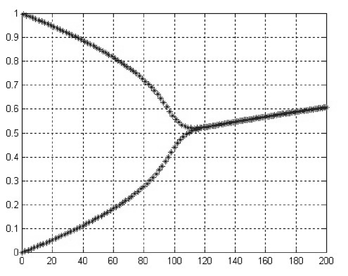
Figure 1. A computer solution, $y=\gamma_{n}^{2}$, of the string equation for the quartic model: $g=1$, $t=-1$, $N=400$.

$\lambda_{c}=\frac{1}{4}$, so that for any $\varepsilon>0$, as $N\to\infty$,

$$\gamma_{n}^{2}=R\left(\frac{n}{N}\right)+O(N^{-1}),\quad{\rm if}\quad\frac{n}{N}\geq\lambda_{c}+\varepsilon,$$ (2.49)

and

$$\gamma_{n}^{2}=\left\{\begin{aligned} &R\left(\frac{n}{N}\right)+O(N^{-1}),\quad n=2k+1,\\ &L\left(\frac{n}{N}\right)+O(N^{-1}),\quad n=2k,\end{aligned}\right.\qquad{\rm if}\quad\frac{n}{N}\leq\lambda_{c}-\varepsilon.$$ (2.50)

The functions $R$ for $\lambda\geq\lambda_{c}$ and $R,L$ for $\lambda\leq\lambda_{c}$ can be found from string equation (2.46):

$$R(\lambda)=\frac{1+\sqrt{1+12\lambda}}{6},\qquad\lambda>\lambda_{c}\,,$$ (2.51)

and

$$R(\lambda),L(\lambda)=\frac{1\pm\sqrt{1-4\lambda}}{2}\,,\qquad\lambda<\lambda_{c}\,.$$ (2.52)

We will discuss below how to justify asymptotics (2.49), (2.50), and their extension for a general $V$.

2.6. Differential equations for the $\psi$-functions.

Define

$$\vec{\Psi}_{n}(z)=\begin{pmatrix}\psi_{n}(z)\\ \psi_{n-1}(z)\end{pmatrix}\,.$$ (2.53)

Then

$$\vec{\Psi}^{\prime}_{n}(z)=NA_{n}(z)\vec{\Psi}_{n}(z),$$ (2.54)

where

$$A_{n}(z)=\begin{pmatrix}-\displaystyle\frac{V^{\prime}(z)}{2}-\gamma_{n}u_{n}(z)&\gamma_{n}v_{n}(z)\\ -\gamma_{n}v_{n-1}(z)&\displaystyle\frac{V^{\prime}(z)}{2}+\gamma_{n}u_{n}(z)\end{pmatrix}$$ (2.55)

and

$$u_{n}(z)=[W(Q,z)]_{n,n-1},\qquad v_{n}(z)=[W(Q,z)]_{nn},$$ (2.56)

where

$$W(Q,z)=\frac{V^{\prime}(Q)-V^{\prime}(z)}{Q-z}\,.$$ (2.57)

Observe that ${{\operatorname{Tr}\,}}A_{n}(z)=0.$

Example. Even quartic model, $V(M)=\frac{t}{2}M^{2}+\frac{g}{4}M^{4}\,.$ Matrix $A_{n}(z)$:

$$A_{n}(z)=\begin{pmatrix}-\frac{1}{2}(tz+gz^{3})-g\gamma_{n}^{2}z&\gamma_{n}(gz^{2}+\theta_{n})\\ -\gamma_{n}(gz^{2}+\theta_{n-1})&\frac{1}{2}(tz+gz^{3})+g\gamma_{n}^{2}z\end{pmatrix}$$ (2.58)

where

$$\theta_{n}=t+g\gamma_{n}^{2}+g\gamma_{n+1}^{2}.$$ (2.59)

2.7. Lax pair for the discrete string equations.

Three term recurrence relation (2.28) can be written as

$$\vec{\Psi}_{n+1}(z)=U_{n}(z)\vec{\Psi}_{n}(z),$$ (2.60)

where

$$U_{n}(z)=\begin{pmatrix}\gamma^{-1}_{n+1}(z-\beta_{n})&-\gamma^{-1}_{n+1}\gamma_{n}\\ 1&0\end{pmatrix}$$ (2.61)

Differential equation (2.54) and recurrence equation (2.60) form the Lax pair for discrete string equations (2.40). This means that the compatibility condition of (2.54) and (2.60),

$$U_{n}^{\prime}=N(A_{n+1}U_{n}-U_{n}A_{n}),$$ (2.62)

when written for the matrix elements, implies (2.40).

3. The Riemann-Hilbert problem for orthogonal polynomials

3.1. Adjoint functions.

Introduce the adjoint functions to $P_{n}(z)$ as

$$Q_{n}(z)=\frac{1}{2\pi i}\int_{-\infty}^{\infty}\frac{P_{n}(u)\,w(u)\,du}{u-z}\,,\quad z\in{\mathbb{C}}\setminus{\mathbb{R}},$$ (3.1)

where

$$w(z)=e^{-NV(z)}$$ (3.2)

is the weight for the orthogonal polynomials $P_{n}$. Define

$$Q_{n\pm}(x)=\lim_{\begin{subarray}{c}z\to x\\ \pm{\operatorname{Im\,}}z>0\end{subarray}}Q_{n}(z),\quad-\infty<x<\infty.$$ (3.3)

Then the well-known formula for the jump of the Cauchy type integral gives that

$$Q_{n+}(x)-Q_{n-}(x)=w(x)P_{n}(x).$$ (3.4)

The asymptotics of $Q_{n}(z)$ as $z\to\infty$, $z\in{\mathbb{C}}$, is given as

$$Q_{n}(z) =\frac{1}{2\pi i}\int_{-\infty}^{\infty}\frac{w(u)P_{n}(u)\,du}{u-z}\cong-\frac{1}{2\pi i}\int_{-\infty}^{\infty}w(u)P_{n}(u)\sum_{j=0}^{\infty}\frac{u^{j}}{z^{j+1}}\,du$$ (3.5)

$$=-\frac{h_{n}}{2\pi iz^{n+1}}+\sum_{j=n+2}^{\infty}\frac{\alpha_{j}}{z^{j}}\,,$$

(due to the orthogonality, the first $n$ terms cancel out). The sign $\cong$ in (3.5) means an asymptotic expansion, so that for any $k\geq n+2$, there exists a constant $C_{k}>0$ such that for all $z\in{\mathbb{C}}$,

$$Q_{n}(z)-\left(-\frac{h_{n}}{2\pi iz^{n+1}}+\sum_{j=n+2}^{k}\frac{\alpha_{j}}{z^{j}}\right)\leq\frac{C_{k}}{(1+|z|)^{k+1}}\,.$$ (3.6)

It can be some doubts in the uniformity of this asymptotics near the real axis, but we assume that the weight $w(z)$ is analytic in a strip $\{z:\;|{\operatorname{Im\,}}z|\leq a\}$, $a>0$, hence the contour of integration in (3.5) can be shifted, and (3.6) holds uniformly in the complex plane.

3.2. The Riemann-Hilbert problem.

Introduce now the matrix-valued function,

$$Y_{n}(z)=\begin{pmatrix}P_{n}(z)&Q_{n}(z)\\ CP_{n-1}(z)&CQ_{n-1}(z)\end{pmatrix},$$ (3.7)

where the constant,

$$C=-\frac{2\pi i}{h_{n-1}}\,,$$ (3.8)

is chosen in such a way that

$$CQ_{n-1}(z)\cong\frac{1}{z^{n}}+\ldots,$$ (3.9)

see (3.5). The function $Y_{n}$ solves the following Riemann-Hilbert problem (RHP):

1. $Y_{n}(z)$ is analytic on ${\mathbb{C}}^{+}\equiv\{{\operatorname{Im\,}}z\geq 0\}$ and ${\mathbb{C}}^{-}\equiv\{{\operatorname{Im\,}}z\leq 0\}$ (two-valued on ${\mathbb{R}}={\mathbb{C}}^{+}\cap{\mathbb{C}}^{-}$).

2. For any real $x$,

   $$Y_{n+}(x)=Y_{n-}(x)j_{Y}(x),\quad j_{Y}(x)=\begin{pmatrix}1&w(x)\\ 0&1\end{pmatrix}.$$ (3.10)

3. As $z\to\infty,$

   $$Y_{n}(z)\cong\left(\displaystyle I+\sum_{k=1}^{\infty}\frac{Y_{k}}{z^{k}}\right)\begin{pmatrix}z^{n}&0\\ 0&z^{-n}\end{pmatrix}$$ (3.11)

   where $Y_{k},\;k=1,2,\dots$, are some constant $2\times 2$ matrices.

Observe that (3.10) follows from (3.4), while (3.11) from (3.9). The RHP (1)–(3) has some nice properties.

First of all, (3.7) is the only solution of the RHP. Let us sketch a proof of the uniqueness. It follows from (3.10), that

$$\det Y_{n+}(x)=\det Y_{n-}(x),$$ (3.12)

hence $\det Y_{n}(z)$ has no jump at the real axis, and hence $Y_{n}(z)$ is an entire function. At infinity, by (3.11),

$$\det Y_{n}(z)\cong 1+\ldots$$ (3.13)

hence

$$\det Y_{n}(z)\equiv 1,$$ (3.14)

by the Liouville theorem. In particular, $Y_{n}(z)$ is invertible for any $z$. Suppose that $\tilde{Y}_{n}$ is another solution of the RHP. Then $X_{n}=\tilde{Y}_{n}Y_{n}^{-1}$ satisfies

$$X_{n+}(x)=\tilde{Y}_{n+}(x)Y_{n+}(x)^{-1}=\tilde{Y}_{n-}(x)j_{Y}(x)j_{Y}(x)^{-1}Y_{n-}^{-1}(x)=X_{n-}(x),$$ (3.15)

hence $X_{n}$ is an entire matrix-valued function. At infinity, by (3.11),

$$X_{n}(z)\cong I+\ldots$$ (3.16)

hence $X_{n}(z)\equiv I$, by the Liouville theorem. This implies that $\tilde{Y}_{n}=Y_{n}$, the uniqueness.

The recurrent coefficients for the orthogonal polynomials can be found as

$$\gamma_{n}^{2}=[Y_{1}]_{21}[Y_{1}]_{12},$$ (3.17)

and

$$\beta_{n-1}=\frac{[Y_{2}]_{21}}{[Y_{1}]_{21}}-[Y_{1}]_{11}\,.$$ (3.18)

Indeed, from (3.7), (3.11),

$$Y_{n}(z)\begin{pmatrix}z^{-n}&0\\ 0&z^{n}\end{pmatrix}=\begin{pmatrix}z^{-n}P_{n}(z)&z^{n}Q_{n}(z)\\ Cz^{-n}P_{n-1}(z)&z^{n}CQ_{n-1}(z)\end{pmatrix}\cong I+\sum_{k=1}^{\infty}\frac{Y_{k}}{z^{k}}\,,$$ (3.19)

hence by (3.5), (3.8), and (2.28),

$$[Y_{1}]_{21}[Y_{1}]_{12}=\left(-\frac{2\pi i}{h_{n-1}}\right)\left(-\frac{h_{n}}{2\pi i}\right)=\frac{h_{n}}{h_{n-1}}=\gamma_{n}^{2},$$ (3.20)

which proves (3.17). Also,

$$\frac{[Y_{2}]_{21}}{[Y_{1}]_{21}}-[Y_{1}]_{11}=p_{n-1,n-2}-p_{n,n-1}\,,$$ (3.21)

where

$$P_{n}(z)=\sum_{j=0}^{n}p_{nj}z^{j}.$$ (3.22)

From (2.28) we obtain that

$$p_{n-1,n-2}-p_{n,n-1}=\beta_{n-1}\,,$$ (3.23)

hence (3.18) follows. The normalizing constant $h_{n}$ can be found as

$$h_{n}=-2\pi i[Y_{1}]_{12},\quad h_{n-1}=-\frac{2\pi i}{[Y_{1}]_{21}}\,.$$ (3.24)

The reproducing kernel $K_{N}(x,y)$ of the eigenvalue correlation functions, see (2.24), is expressed in terms of $Y_{N+}(x)$ as follows:

$$K_{N}(x,y)=e^{-\frac{NV(x)}{2}}e^{-\frac{NV(y)}{2}}\frac{1}{2\pi i(x-y)}\begin{pmatrix}0&1\end{pmatrix}Y_{N+}^{-1}(y)Y_{N+}(x)\begin{pmatrix}1\\ 0\end{pmatrix}.$$ (3.25)

Indeed, by (2.31),

$$K_{N}(x,y) =\gamma_{N}\frac{\psi_{N}(x)\psi_{N-1}(y)-\psi_{N-1}(x)\psi_{N}(y)}{x-y}$$ (3.26)

$$=e^{-\frac{NV(x)}{2}}e^{-\frac{NV(y)}{2}}\frac{\gamma_{N}}{\sqrt{h_{N}h_{N-1}}}\,\frac{P_{N}(x)P_{N-1}(y)-P_{N-1}(x)P_{N}(y)}{x-y}\,.$$

From (3.7), (3.8) and (3.14), we obtain that

$$\begin{pmatrix}0&1\end{pmatrix}Y_{N+}^{-1}(y)Y_{N+}(x)\begin{pmatrix}1\\ 0\end{pmatrix}=\frac{2\pi i}{h_{N-1}}\left[P_{N}(x)P_{N-1}(y)-P_{N-1}(x)P_{N}(y)\right].$$ (3.27)

Also,

$$\frac{\gamma_{N}}{\sqrt{h_{N}h_{N-1}}}=\frac{1}{h_{N-1}},$$ (3.28)

hence equation (3.25) follows.

4. Distribution of eigenvalues and equilibrium measure

4.1. Heuristics.

We begin with some heuristic considerations to explain why we expect that the limiting distribution of eigenvalues solves a variational problem. Let us rewrite (2.17) as

$$d\mu_{N}(\lambda)=\tilde{Z}_{N}^{-1}e^{-H_{N}(\lambda)}d\lambda,$$ (4.1)

where

$$H_{N}(\lambda)=-\sum_{j\not=k}\ln|\lambda_{j}-\lambda_{k}|+N\sum_{j=1}^{N}V(\lambda_{j}).$$ (4.2)

Given $\lambda$, introduce the probability measure on ${\mathbb{R}}^{1}$,

$$d\nu_{\lambda}(x)=N^{-1}\displaystyle\sum_{j=1}^{N}\delta(x-\lambda_{j})dx.$$ (4.3)

Then (4.2) can be rewritten as

$$H_{N}(\lambda)=N^{2}\left[-\iint_{x\not=y}\ln|x-y|d\nu_{\lambda}(x)d\nu_{\lambda}(y)+\int V(x)d\nu_{\lambda}(x)\right].$$ (4.4)

Let $\nu$ be an arbitrary probability measure on ${\mathbb{R}}^{1}$. Set

$$I_{V}(\nu)=-\iint_{x\not=y}\ln|x-y|d\nu(x)d\nu(y)+\int V(x)d\nu(x).$$ (4.5)

Then (4.1) reads

$$d\mu_{N}(\lambda)=\tilde{Z}_{N}^{-1}e^{-N^{2}I_{V}(\nu_{\lambda})}d\lambda.$$ (4.6)

Because of the factor $N^{2}$ in the exponent, we expect that for large $N$ the measure $\mu_{N}$ is concentrated near the minimum of the functional $I_{V}$, i.e. near the equilibrium measure $\nu_{V}$.

4.2. Equilibrium measure.

Consider the minimization problem

$$E_{V}=\inf_{\nu\in M_{1}({\mathbb{R}})}I_{V}(\nu),$$ (4.7)

where

$$M_{1}({\mathbb{R}})=\left\{\nu\,:\,\nu\geq 0,\;\int_{{\mathbb{R}}}d\nu=1\right\},$$ (4.8)

the set of probability measures on the line.

Proposition 4.1.

(See [DKM].) The infinum of $I_{V}(\nu)$ is attained uniquely at a measure $\nu=\nu_{V}$, which is called an equilibrium measure. The measure $\nu_{V}$ is absolutely continuous, and it is supported by a finite union of intervals, $J=\cup_{j=1}^{q}[a_{j},b_{j}]$. On the support, its density has the form

$$p_{V}(x)\equiv\frac{d\nu_{V}}{dx}(x)=\frac{1}{2\pi i}h(x)R^{1/2}_{+}(x),\qquad R(x)=\prod_{j=1}^{q}(x-a_{j})(x-b_{j}).$$ (4.9)

Here $R^{1/2}(x)$ is the branch with cuts on $J$, which is positive for large positive $x$, and $R_{+}^{1/2}(x)$ is the value of $R^{1/2}(x)$ on the upper part of the cut. The function $h(x)$ is a polynomial, which is the polynomial part of the function $\frac{V^{\prime}(x)}{R^{1/2}(x)}$ at infinity, i.e.

$$\frac{V^{\prime}(x)}{R^{1/2}(x)}=h(x)+O(x^{-1}).$$ (4.10)

In particular, $\deg h=\deg V-1-q$.

There is a useful formula for the equilibrium density [DKM]:

$$\frac{d\nu_{V}(x)}{dx}=\frac{1}{\pi}\sqrt{q(x)},$$ (4.11)

where

$$q(x)=-\left(\frac{V^{\prime}(x)}{2}\right)^{2}+\int\frac{V^{\prime}(x)-V^{\prime}(y)}{x-y}d\nu_{V}(y).$$ (4.12)

This, in fact, is an equation on $q$, since the right-hand side contains an integration with respect to $\nu_{V}$. Nevertheless, if $V$ is a polynomial of degree $p=2p_{0}$, then (4.12) determines uniquely more then a half of the coefficients of the polynomial $q$,

$$q(x)=-\left(\frac{V^{\prime}(x)}{2}\right)^{2}-O(x^{p-2}).$$ (4.13)

Example. If $V(x)$ is convex then $\nu_{V}$ is regular, and the support of $\nu_{V}$ consists of a single interval, see e.g. [KuM1]. For the Gaussian ensemble, $V(x)=x^{2}$, hence, by (4.13), $q(x)=a^{2}-x^{2}$. Since

$$\int_{-a}^{a}\frac{1}{\pi}\sqrt{a^{2}-x^{2}}\,dx=1,$$

we find that $a=\sqrt{2}$, hence

$$p_{V}(x)=\frac{1}{\pi}\sqrt{2-x^{2}}\,,\qquad|x|\leq\sqrt{2},$$ (4.14)

the Wigner semicircle law.

4.3. The Euler-Lagrange variational conditions.

A nice and important property of minimization problem (4.7) is that the minimizer is uniquely determined by the Euler-Lagrange variational conditions: for some real constant $l$,

$$2\int_{{\mathbb{R}}}\log|x-y|d\nu(y)-V(x)=l,\;\text{for}\;x\in J,$$ (4.15)

$$2\int_{{\mathbb{R}}}\log|x-y|d\nu(y)-V(x)\leq l,\;\text{for}\;x\in{\mathbb{R}}\setminus J,$$ (4.16)

see [DKM].

Definition. (See [DKMVZ2].) The equilibrium measure,

$$d\nu_{V}(x)=\frac{1}{2\pi i}h(x)R^{1/2}_{+}(x)\,dx$$ (4.17)

is called regular (otherwise singular) if

1. $h(x)\not=0$ on the (closed) set $J$.

2. Inequality (4.16) is strict,

   $$2\int\log|x-y|d\nu_{V}(y)-V(x)<l,\;\text{\rm for}\;x\in{\mathbb{R}}\setminus J.$$ (4.18)

4.4. Construction of the equilibrium measure: equations on the end-points.

The strategy to construct the equilibrium measure is the following: first we find the end-points of the support, and then we use equation (4.10) to find $h(x)$ and hence the density. The number $q$ of cuts is not, in general, known, and we try different $q$’s. Consider the resolvent,

$$\omega(z)=\int_{J}\frac{d\nu_{V}(x)}{z-x},\quad z\in{\mathbb{C}}\setminus J.$$ (4.19)

The Euler-Lagrange variational condition implies that

$$\omega(z)=\frac{V^{\prime}(z)}{2}-\frac{h(z)R^{1/2}(z)}{2}\,.$$ (4.20)

Observe that as $z\to\infty$,

$$\omega(z)=\frac{1}{z}+\frac{m_{1}}{z^{2}}+\dots,\quad m_{k}=\int_{J}x^{k}\rho(x)dx.$$ (4.21)

The equation

$$\frac{V^{\prime}(z)}{2}-\frac{h(z)R^{1/2}(z)}{2}=\frac{1}{z}+O(z^{-2})\,.$$ (4.22)

gives $q+1$ equation on $a_{1},b_{1},\dots,a_{q},b_{q}$, if we substitute formula (4.10) for $h$. Remaining $q-1$ equation are

$$\int_{b_{j}}^{a_{j+1}}h(x)R^{1/2}(x)\,dx=0,\quad j=1,\dots,q-1,$$ (4.23)

which follow from (4.20) and (4.15).

Example. Even quartic model, $V(M)=\frac{t}{2}M^{2}+\frac{1}{4}M^{4}$. For $t\geq t_{c}=-2$, the support of the equilibrium distribution consists of one interval $[-a,a]$ where

$$a=\left(\frac{-2t+2\left(t^{2}+12\right)^{1/2}}{3}\right)^{1/2}$$ (4.24)

and

$$p_{V}(x)=\frac{1}{\pi}\left(c+\frac{1}{2}x^{2}\right)\sqrt{a^{2}-x^{2}}$$ (4.25)

where

$$c=\frac{t+\left((t^{2}/4)+3\right)^{1/2}}{3}\,.$$ (4.26)

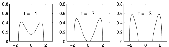
Figure 2. The density function, $p_{V}(x)$, for the even quartic potential, $V(M)=\frac{t}{2}M^{2}+\frac{1}{4}M^{4}$, for $t=-1,-2,-3$.

In particular, for $t=-2$,

$$p_{V}(x)=\frac{1}{2\pi}x^{2}\sqrt{4-x^{2}}$$ (4.27)

For $t<-2$, the support consists of two intervals, $[-a,-b]$ and $[b,a]$, where

$$a=\sqrt{2-t},\quad b=\sqrt{-2-t}\,,$$ (4.28)

and

$$p_{V}(x)=\frac{1}{2\pi}|x|\sqrt{(a^{2}-x^{2})(x^{2}-b^{2})}\,.$$ (4.29)

Fig.2 shows the density function for the even quartic potential, for $t=-1,-2,-3$.

Lecture 2. Large $N$ asymptotics of orthogonal polynomials. The Riemann-Hilbert approach

In this lecture we present the Riemann-Hilbert approach to the large $N$ asymptotics of orthogonal polynomials. The central point of this approach is a construction of an asymptotic solution to the RHP, as $N\to\infty$. We call such a solution, a parametrix. In the original paper of Bleher and Its [BI1] the RH approach was developed for an even quartic polynomial $V(M)$ via a semiclassical solution of the differential equation for orthogonal polynomials. Then, in a series of papers, Deift, Kriecherbauer, McLaughlin, Venakides, and Zhou [DKM], [DKMVZ1], [DKMVZ2] developed the RH approach for a general real analytic $V$, with some conditions on the growth at infinity. The DKMVZ-approach is based on the Deift-Zhou steepest descent method, see [DZ]. In this lecture we present the main steps of the DKMVZ-approach. For the sake of simplicity, we will assume that $V$ is regular. In this approach a sequence of transformations of the RHP is constructed, which reduces the RHP to a simple RHP which can be solved by a series of perturbation theory. This sequence of transformations gives the parametrix of the RHP in different regions on complex plane. The motivation for the first transformation comes from the Heine formula for orthogonal polynomials.

5. Heine’s formula for orthogonal polynomials.

The Heine formula, see, e.g., [Sze], gives the $N$-th orthogonal polynomial as the matrix integral,

$$P_{N}(z)=\left\langle\det(z-M)\right\rangle\equiv Z_{N}^{-1}\int_{\mathcal{H}_{N}}\det(z-M)e^{-N{{\operatorname{Tr}\,}}V(M)}dM.$$ (5.1)

In the ensemble of eigenvalues,

$$P_{N}(z)=\left\langle\prod_{j=1}^{N}(z-\lambda_{j})\right\rangle\equiv\tilde{Z}_{N}^{-1}\int\prod_{j=1}^{N}(z-\lambda_{j})\prod_{j>k}(\lambda_{j}-\lambda_{k})^{2}\prod_{j=1}^{N}e^{-NV(\lambda_{j})}d\lambda$$ (5.2)

Since $\nu_{\lambda}$ is close to the equilibrium measure $\nu$ for typical $\lambda$, we expect that

$$N^{-1}\log\left\langle\prod_{j=1}^{N}(z-\lambda_{j})\right\rangle\approx\int_{J}\log(z-x)d\nu_{V}(x),$$

hence by the Heine formula,

$$N^{-1}\log P_{N}(z)\approx\int_{J}\log(z-x)d\nu_{V}(x).$$ (5.3)

This gives a heuristic semiclassical approximation for the orthogonal polynomial,

$$P_{N}(z)\approx\exp\left[N\int_{J}\log(z-x)d\nu_{V}(x)\right],$$ (5.4)

and it motivates the introduction of the “$g$-function”.

5.1. $g$-function

Define the $g$-function as

$$g(z)=\int_{J}\log(z-x)d\nu_{V}(x),\quad z\in{\mathbb{C}}\setminus(-\infty,b_{q}],$$ (5.5)

where we take the principal branch for logarithm.

Properties of $g(z)$:

1. $g(z)$ is analytic in ${\mathbb{C}}\setminus(-\infty,b_{q}]$.

2. As $z\to\infty$

   $$g(z)=\log z-\sum_{j=1}^{\infty}\frac{g_{j}}{z^{j}}\,,\qquad g_{j}=\int_{J}\frac{x^{j}}{j}\,d\nu_{V}(x).$$ (5.6)

3. By (4.19), (4.20),

   $$g^{\prime}(z)=\omega(z)=\frac{V^{\prime}(z)}{2}-\frac{h(z)R^{1/2}(z)}{2}\,.$$ (5.7)

4. By (4.15),

   $$g_{+}(x)+g_{-}(x)=V(x)+l,\quad x\in J.$$ (5.8)

5. By (4.18),

   $$g_{+}(x)+g_{-}(x)<V(x)+l,\quad x\in{\mathbb{R}}\setminus J.$$ (5.9)

6. Equation (5.5) implies that the function

   $$G(x)\equiv g_{+}(x)-g_{-}(x)$$ (5.10)

   is pure imaginary for all real $x$, and $G(x)$ is constant in each component of ${\mathbb{R}}\setminus J$,

   $$G(x)=i\Omega_{j}\;\text{ for}\;b_{j}<x<a_{j+1},\quad 1\leq j\leq q-1,$$ (5.11)

   where

   $$\Omega_{j}=2\pi\sum_{k=j+1}^{q}\int_{a_{k}}^{b_{k}}p_{V}(x)\,dx,\quad 1\leq j\leq q-1.$$ (5.12)

7. Also,

   $$G(x)=i\Omega_{j}-2\pi i\int_{b_{j}}^{x}p_{V}(s)\,ds\;\text{ for}\;a_{j}<x<b_{j},\quad 1\leq j\leq q,$$ (5.13)

   where we set $\Omega_{q}=0$.

Observe that from (5.13) and (4.9) we obtain that $G(x)$ is analytic on $(a_{j},b_{j})$, and

$$\left.\frac{dG(x+iy)}{dy}\right|_{y=0}=2\pi p_{V}(x)>0,\quad x\in(a_{j},b_{j}),\quad 1\leq j\leq q.$$ (5.14)

From (5.8) we have also that

$$G(x)=2g_{+}(x)-V(x)-l=-[2g_{-}(x)-V(x)-l],\quad x\in J.$$ (5.15)

6. First Transformation of the RH Problem

Our goal is to construct an asymptotic solution to RHP (3.10), (3.11) for $Y_{N}(z)$, as $N\to\infty$. In our construction we will assume that the equilibrium measure $\nu_{V}$ is regular. By (5.4) we expect that

$$P_{N}(z)\approx e^{Ng(z)},$$ (6.1)

therefore, we make the following substitution in the RHP:

$$Y_{N}(z)=e^{\frac{Nl}{2}\sigma_{3}}T_{N}(z)e^{N\left[g(z)-\frac{l}{2}\right]\sigma_{3}},\qquad\sigma_{3}=\begin{pmatrix}1&0\\ 0&-1\end{pmatrix}.$$ (6.2)

Then $T_{N}(z)$ solves the following RH problem:

1. $T_{N}(z)$ is analytic in ${\mathbb{C}}\setminus{\mathbb{R}}$.

2. $T_{N+}(x)=T_{N-}(x)j_{T}(x)$ for $x\in{\mathbb{R}}$, where

   $$j_{T}(x)=\begin{pmatrix}e^{-N[g_{+}(x)-g_{-}(x)]}&e^{N[g_{+}(x)+g_{-}(x)-V(x)-l]}\\ 0&e^{N[g_{+}(x)-g_{-}(x)]}\end{pmatrix}.$$ (6.3)

3. $T_{N}(z)=I+O(z^{-1})$, as $z\to\infty$.

The above properties of $g(z)$ ensure the following properties of the jump matrix $j_{T}$:

1. $j_{T}(x)$ is exponentially close to the identity matrix on $(-\infty,a_{1})\cup(b_{q},\infty)$. Namely,

   $$j_{T}(x)=\begin{pmatrix}1&O(e^{-Nc(x)})\\ 0&1\end{pmatrix},\quad x\in(-\infty,a_{1})\cup(b_{q},\infty),$$ (6.4)

   where $c(x)>0$ is a continuous function such that

   $$\lim_{x\to\pm\infty}\frac{c(x)}{\ln|x|}=\infty,\quad\lim_{x\to a_{1}}c(x)=\lim_{x\to b_{q}}c(x)=0.$$ (6.5)

2. For $1\leq j\leq q-1$,

   $$j_{T}(x)=\begin{pmatrix}e^{-iN\Omega_{j}}&O(e^{-Nc(x)})\\ 0&e^{iN\Omega_{j}}\end{pmatrix},\quad x\in(b_{j},a_{j+1}),$$ (6.6)

   where $c(x)>0$ is a continuous function such that

   $$\lim_{x\to b_{j}}c(x)=\lim_{x\to a_{j+1}}c(x)=0.$$ (6.7)

3. On $J$,

   $$j_{T}(x)=\begin{pmatrix}e^{-NG(x)}&1\\ 0&e^{NG(x)}\end{pmatrix}\,.$$ (6.8)

The latter matrix can be factorized as follows:

$$\begin{pmatrix}e^{-NG(x)}&1\\ 0&e^{NG(x)}\end{pmatrix} =\begin{pmatrix}1&0\\ e^{NG(x)}&1\end{pmatrix}\begin{pmatrix}0&1\\ -1&0\end{pmatrix}\begin{pmatrix}1&0\\ e^{-NG(x)}&1\end{pmatrix}$$ (6.9)

$$\equiv j_{-}(x)j_{M}j_{+}(x),$$

This leads to the second transformation of the RHP.

7. Second transformation of the RHP: Opening of lenses

The function $e^{-NG(x)}$ is analytic on each open interval $(a_{j},b_{j})$. Observe that $|e^{-NG(x)}|=1$ for real $x\in(a_{j},b_{j})$, and $e^{-NG(z)}$ is exponentially decaying for ${\operatorname{Im\,}}z>0$. More precisely, by (5.14), there exists $y_{0}>0$ such that $e^{-NG(z)}$ satisfies the estimate,

$$|e^{-NG(z)}|\leq e^{-Nc(z)},\quad z\in R_{j}^{+}=\{z=x+iy:\;a_{j}<x<b_{j},\;0<y<y_{0}\},$$ (7.1)

where $c(z)>0$ is a continuous function in $R_{j}^{+}$. Observe that $c(z)\to 0$ as ${\operatorname{Im\,}}z\to 0$. In addition, $|e^{NG(z)}|=|e^{-NG(\bar{z})}|$, hence

$$|e^{NG(z)}|\leq e^{-Nc(z)},\quad z\in R_{j}^{-}=\{z=x+iy:\;a_{j}<x<b_{j},\;0<-y<y_{0}\},$$ (7.2)

where $c(z)=c(\bar{z})>0$. Consider a $C^{\infty}$ curve $\gamma_{j}^{+}$ from $a_{j}$ to $b_{j}$ such that

$$\gamma_{j}^{+}=\{x+iy:\;y=f_{j}(x)\},$$ (7.3)

where $f_{j}(x)$ is a $C^{\infty}$ function on $[a_{j},b_{j}]$ such that

$$f_{j}(a_{j})=f_{j}(b_{j})=0;\quad f^{\prime}_{j}(a_{j})=-f^{\prime}(b_{j})=\sqrt{3};\quad 0<f_{j}(x)<y_{0},\quad a_{j}<x<b_{j}.$$ (7.4)

Consider the conjugate curve,

$$\gamma_{j}^{-}=\overline{\gamma_{j}^{+}}=\{x-iy:\;y=f_{j}(x)\},$$ (7.5)

see Fig.3.

Figure 3. The lenses.

The region bounded by the interval $[a_{j},b_{j}]$ and $\gamma_{j}^{+}$ ($\gamma_{j}^{-}$) is called the upper (lower) lens, $\mathcal{L}_{j}^{\pm}$, respectively. Define for $j=1,\ldots,q$,

$$S_{N}(z)=\left\{\begin{aligned} {}&T_{N}(z)j_{+}^{-1}(z),\quad\text{if $z$ is in the upper lens, $z\in\mathcal{L}_{j}^{+}$},\\ {}&T_{N}(z)j_{-}(z),\quad\text{if $z$ is in the lower lens, $z\in\mathcal{L}_{j}^{-}$},\\ {}&T_{N}(z)\quad\text{otherwise,}\end{aligned}\right.$$ (7.6)

where

$$j_{\pm}(z)=\begin{pmatrix}1&0\\ e^{\mp NG(z)}&1\end{pmatrix}.$$ (7.7)

Then $S_{N}(z)$ solves the following RH problem:

1. $S_{N}(z)$ is analytic in ${\mathbb{C}}\setminus({\mathbb{R}}\cup\Gamma)$, $\Gamma=\gamma_{1}^{+}\cup\gamma_{1}^{-}\cup\dots\cup\gamma_{q}^{+}\cup\gamma_{q}^{-}$.

2. $$S_{N+}(z)=S_{N-}(z)j_{S}(z),\quad z\in{\mathbb{R}}\cup\gamma,$$ (7.8)

   where the jump matrix $j_{S}(z)$ has the following properties:

   1. $j_{S}(z)=\begin{pmatrix}0&1\\ -1&0\end{pmatrix}$ for $z\in J$.

   2. $j_{S}(z)=j_{T}(z)=\begin{pmatrix}e^{-iN\Omega_{j}}&O(e^{-c(x)N})\\ 0&e^{iN\Omega_{j}}\end{pmatrix}$ for $z\in(b_{j},a_{j+1})$, $j=1,\ldots,q-1$, and $j_{S}(z)=j_{T}(z)=\begin{pmatrix}1&O(e^{-c(x)N})\\ 0&1\end{pmatrix}$ for $z\in(-\infty,a_{1})\cup(b_{q},\infty).$

   3. $j_{S}(z)=j_{\pm}(z)=\begin{pmatrix}1&0\\ O(e^{-c(z)N})&1\end{pmatrix}$ for $z\in\gamma_{j}^{\pm}$, $j=1,\ldots,q$, where $c(z)>0$ is a continuous function such that $c(z)\to 0$ as $z\to a_{j},b_{j}$.

3. $S_{N}(z)=I+O(z^{-1})$, as $z\to\infty$.

We expect, and this will be justified later, that as $N\to\infty$, $S_{N}(z)$ converges to a solution of the model RHP, in which we drop the $O(e^{-cN})$-terms in the jump matrix $j_{S}(z)$. Let us consider the model RHP.

8. Model RHP

We are looking for $M(z)$ that solves the following model RHP:

1. $M(z)$ is analytic in ${\mathbb{C}}\setminus[a_{1},b_{q}]$,

2. $$M_{+}(z)=M_{-}(z)j_{M}(z),\quad z\in[a_{1},b_{q}],$$ (8.1)

   where the jump matrix $j_{M}(z)$ is given by the following formulas:

   1. $j_{M}(z)=\begin{pmatrix}0&1\\ -1&0\end{pmatrix}$ for $z\in J$

   2. $j_{M}(z)=\begin{pmatrix}e^{-iN\Omega_{j}}&0\\ 0&e^{iN\Omega_{j}}\end{pmatrix}$ for $z\in[b_{j},a_{j+1}]$, $j=1,\ldots,q-1$.

3. $M(z)=I+O(z^{-1})$, as $z\to\infty$.

We will construct a solution to the model RHP by following the work [DKMVZ2].

8.1. Solution of the model RHP. One-cut case

Assume that $J$ consist of a single interval $[a,b]$. Then the model RH problem reduces to the following:

1. $M(z)$ is analytic in ${\mathbb{C}}\setminus[a,b]$,

2. $M_{+}(z)=M_{-}(z)\begin{pmatrix}0&1\\ -1&0\end{pmatrix}$ for $z\in[a,b]$.

3. $M(z)=I+O(z^{-1})$, as $z\to\infty$.

This RHP can be reduced to a pair of scalar RH problems. We have that

$$\begin{pmatrix}0&1\\ -1&0\end{pmatrix}=\frac{1}{2}\begin{pmatrix}1&1\\ i&-i\end{pmatrix}\begin{pmatrix}i&0\\ 0&-i\end{pmatrix}\begin{pmatrix}1&-i\\ 1&i\end{pmatrix}$$ (8.2)

Let

$$\tilde{M}(z)=\frac{1}{2}\begin{pmatrix}1&-i\\ 1&i\end{pmatrix}M(z)\begin{pmatrix}1&1\\ i&-i\end{pmatrix}.$$ (8.3)

Then $\tilde{M}(z)$ solves the following RHP:

1. $\tilde{M}(z)$ is analytic in ${\mathbb{C}}\setminus[a,b]$,

2. $\tilde{M}_{+}(z)=\tilde{M}_{-}(z)\begin{pmatrix}i&0\\ 0&-i\end{pmatrix}$ for $z\in[a,b]$.

3. $\tilde{M}(z)=I+O(z^{-1})$, as $z\to\infty$.

This is a pair of scalar RH problems, which can be solved by the Cauchy integral:

$$\tilde{M}(z) =\begin{pmatrix}e^{\frac{1}{2\pi i}\int_{a}^{b}\frac{\log i}{s-z}ds}&0\\ 0&e^{\frac{1}{2\pi i}\int_{a}^{b}\frac{\log(-i)}{s-z}ds}\end{pmatrix}=\begin{pmatrix}e^{\frac{1}{4}\log\frac{z-b}{z-a}}&0\\ 0&e^{-\frac{1}{4}\log\frac{z-b}{z-a}}\end{pmatrix}=\begin{pmatrix}\gamma^{-1}&0\\ 0&\gamma\end{pmatrix},$$ (8.4)

where

$$\gamma(z)=\left(\frac{z-a}{z-b}\right)^{1/4}$$ (8.5)

with cut on $[a,b]$ and the branch such that $\gamma(\infty)=1$. Thus,

$$M(z)=\frac{1}{2}\begin{pmatrix}1&1\\ i&-i\end{pmatrix}\begin{pmatrix}\gamma^{-1}&0\\ 0&\gamma\end{pmatrix}\begin{pmatrix}1&1\\ i&-i\end{pmatrix}^{-1}=\begin{pmatrix}\frac{\gamma(z)+\gamma^{-1}(z)}{2}&\frac{\gamma(z)-\gamma^{-1}(z)}{(-2i)}\\ \frac{\gamma(z)-\gamma^{-1}(z)}{2i}&\frac{\gamma(z)+\gamma^{-1}(z)}{2}\end{pmatrix},$$ (8.6)

$$\det M(z)=1.$$

At infinity we have

$$\gamma(z)=1+\frac{b-a}{4z}+O(z^{-2}),$$ (8.7)

hence

$$M(z)=I+\frac{1}{z}\begin{pmatrix}0&\frac{b-a}{(-4i)}\\ \frac{b-a}{4i}&0\end{pmatrix}+O(z^{-2}).$$ (8.8)

8.2. Solution of the model RHP. Multicut case

This will be done in three steps.

Step 1. Consider the auxiliary RHP,

1. $Q(z)$ is analytic in ${\mathbb{C}}\setminus J$, $J=\cup_{j=1}^{q}[a_{j},b_{j}]$,

2. $Q_{+}(z)=Q_{-}(z)\begin{pmatrix}0&1\\ -1&0\end{pmatrix}$ for $z\in J$.

3. $Q(z)=I+O(z^{-1})$, as $z\to\infty$.

Then, similar to the one-cut case, this RHP is reduced to two scalar RHPs, and the solution is

$$Q(z)=\begin{pmatrix}\frac{\gamma(z)+\gamma^{-1}(z)}{2}&\frac{\gamma(z)-\gamma^{-1}(z)}{(-2i)}\\ \frac{\gamma(z)-\gamma^{-1}(z)}{2i}&\frac{\gamma(z)+\gamma^{-1}(z)}{2}\end{pmatrix},$$ (8.9)

where

$$\gamma(z)=\prod_{j=1}^{q}\left(\frac{z-a_{j}}{z-b_{j}}\right)^{1/4},\qquad\gamma(\infty)=1,$$ (8.10)

with cuts on $J$. At infinity we have

$$\gamma(z)=1+\sum_{j=1}^{q}\frac{b_{j}-a_{j}}{4z}+O(z^{-2}),$$ (8.11)

hence

$$Q(z)=I+\frac{1}{z}\begin{pmatrix}0&\sum_{j=1}^{q}\frac{b_{j}-a_{j}}{(-4i)}\\ \sum_{j=1}^{q}\frac{b_{j}-a_{j}}{4i}&0\end{pmatrix}+O(z^{-2}).$$ (8.12)

In what follows, we will modify this solution to satisfy part (b) in jump matrix in (8.1). This requires some Riemannian geometry and the theta function.

Step 2. Let $X$ be the two-sheeted Riemannian surface of the genus

$$g=q-1,$$ (8.13)

associated to $\sqrt{R(z)}$, where

$$R(z)=\prod_{j=1}^{q}(z-a_{j})(z-b_{j}),$$ (8.14)

Figure 4. The Riemannian surface associated to $\sqrt{R(z)}$.

with cuts on the intervals $(a_{j},b_{j})$, $j=1,\ldots,q$, see Fig.4. We fix the first sheet of $X$ by the condition that on this sheet,

$$\sqrt{R(x)}>0,\qquad x>b_{q}.$$ (8.15)

We would like to introduce $2g$ cycles on $X$, forming a homology basis. To that end, consider, for $j=1,\ldots,g$, a cycle $A_{j}$ on $X$, which goes around the interval $(b_{j},a_{j+1})$ in the negative direction, such that the part of $A_{j}$ in the upper half-plane, $A_{j}^{+}\equiv A_{j}\cup\{z:\;{\operatorname{Im\,}}z\geq 0\}$, lies on the first sheet of $X$, and the one in the lower half-plane, $A_{j}^{-}\equiv A_{j}\cup\{z:\;{\operatorname{Im\,}}z\leq 0\}$, lies on the second sheet, $j=1,\ldots,g$. In addition, consider a cycle $B_{j}$ on $X$, which goes around the interval $(a_{1},b_{j})$ on the first sheet in the negative direction,

Figure 5. The basis of cycles on $X$.

see Fig.5. Then the cycles $(A_{1},\ldots,A_{g},B_{1},\ldots,B_{g})$ form a canonical homology basis for $X$.

Consider the linear space $\Omega$ of holomorphic one-forms on $X$,

$$\Omega=\left\{\omega=\sum_{j=0}^{q-2}\frac{c_{j}z^{j}dz}{\sqrt{R(z)}}\right\}.$$ (8.16)

The dimension of $\Omega$ is equal to $g$. Consider the basis in $\Omega$,

$$\omega=(\omega_{1},\ldots,\omega_{g}),$$

with normalization

$$\int_{A_{j}}\omega_{k}=\delta_{jk},\qquad j,k=1,\ldots,g.$$ (8.17)

Such a basis exists and it is unique, see [FK]. Observe that the numbers

$$m_{jk}=\int_{A_{j}}\frac{z^{k}dz}{\sqrt{R(z)}}=2\int_{b_{j}}^{a_{j+1}}\frac{x^{k}dx}{\sqrt{R(x)}}\,,\qquad 1\leq j\leq g,\quad 1\leq k\leq g-1,$$ (8.18)

are real. This implies that the basis $\omega$ is real, i.e., the one-forms,

$$\omega_{j}=\sum_{k=0}^{g-1}\frac{c_{jk}z^{k}dz}{\sqrt{R(z)}},$$ (8.19)

have real coefficients $c_{jk}$.

Define the associated Riemann matrix of $B$-periods,

$$\tau=(\tau_{jk}),\qquad\tau_{jk}=\int_{B_{j}}\omega_{k},\qquad j,k=1,\ldots,g.$$ (8.20)

Since $\sqrt{R(x)}$ is pure imaginary on $(a_{j},b_{j})$, the numbers $\tau_{jk}$ are pure imaginary. It is known, see, e.g., [FK], that the matrix $\tau$ is symmetric and $(-i\tau)$ is positive definite.

The Riemann theta function with the matrix $\tau$ is defined as

$$\theta(s)=\sum_{m\in{\mathbb{Z}}^{g}}e^{2\pi i(m,s)+\pi i(m,\tau m)},\quad s\in{\mathbb{C}}^{g};\qquad(m,s)=\sum_{j=1}^{g}m_{j}s_{j}.$$ (8.21)

The quadratic form $i(m,\tau m)$ is negative definite, hence the series is absolutely convergent and $\theta(s)$ is analytic in ${\mathbb{C}}^{g}$. The theta function is an even function,

$$\theta(-s)=\theta(s),$$ (8.22)

and it has the following periodicity properties:

$$\theta(s+e_{j})=\theta(s);\qquad\theta(s+\tau_{j})=e^{-2\pi is_{j}-\pi i\tau_{jj}}\theta(s),$$ (8.23)

where $e_{j}=(0,\ldots,0,1,0,\ldots,0)$ is the $j$-th basis vector in ${\mathbb{C}}^{g}$, and $\tau_{j}=\tau e_{j}$. This implies that the function

$$f(s)=\frac{\theta(s+d+c)}{\theta(s+d)},$$ (8.24)

where $c,d\in{\mathbb{C}}^{g}$ are arbitrary constant vectors, has the periodicity properties,

$$f(s+e_{j})=f(s);\qquad f(s+\tau_{j})=e^{-2\pi ic_{j}}f(s).$$ (8.25)

Consider now the theta function associated with the Riemann surface $X$. It is defined as follows. Introduce the vector function,

$$u(z)=\int_{b_{q}}^{z}\omega,\qquad z\in{\mathbb{C}}\setminus(a_{1},b_{q}),$$ (8.26)

where $\omega$ is the basis of holomorphic one-forms, determined by equations (8.17). The contour of integration in (8.26) lies in ${\mathbb{C}}\setminus(a_{1},b_{q})$, on the first sheet of $X$. We will consider $u(z)$ as a function with values in ${\mathbb{C}}^{g}/{\mathbb{Z}}^{g}$,

$$u:\;{\mathbb{C}}\setminus(a_{1},b_{q})\to{\mathbb{C}}^{g}/{\mathbb{Z}}^{g}\,.$$ (8.27)

On $[a_{1},b_{q}]$ the function $u(z)$ is two-valued. From (8.20) we have that

$$u_{+}(x)-u_{-}(x)=\tau_{j},\quad x\in[b_{j},a_{j+1}];\qquad 1\leq j\leq q-1.$$ (8.28)

Since $\sqrt{R(x)}_{-}=-\sqrt{R(x)}_{+}$ on $[a_{j},b_{j}]$, we have that the function $u_{+}(x)+u_{-}(x)$ is constant on $[a_{j},b_{j}]$. It follows from (8.17) that $\mod{\mathbb{Z}}^{q}$,

$$u_{+}(b_{j})+u_{-}(b_{j})=u_{+}(a_{j+1})+u_{-}(a_{j+1}),\qquad 1\leq j\leq q-1$$ (8.29)

Since $u_{+}(b_{q})=u_{-}(b_{q})=0$, we obtain that

$$u_{+}(x)+u_{-}(x)=0,\quad x\in J=\bigcup_{j=1}^{q}[a_{j},b_{j}].$$ (8.30)

Define

$$f_{1}(z)=\frac{\theta(u(z)+d+c)}{\theta(u(z)+d)},\quad f_{2}(z)=\frac{\theta(-u(z)+d+c)}{\theta(-u(z)+d)},\qquad z\in{\mathbb{C}}\setminus(a_{1},b_{q}),$$ (8.31)

where $c,d\in{\mathbb{C}}^{g}$ are arbitrary constant vectors. Then from (8.28) and (8.25) we obtain that for $1\leq j\leq q-1$,

$$f_{1}(x+i0)=e^{-2\pi ic_{j}}f_{1}(x-i0),\quad f_{2}(x+i0)=e^{2\pi ic_{j}}f_{2}(x-i0),\quad x\in(b_{j},a_{j+1}),$$ (8.32)

and from (8.30) that

$$f_{1}(x+i0)=f_{2}(x-i0),\quad f_{2}(x+i0)=f_{1}(x-i0),\quad x\in J.$$ (8.33)

Let us take

$$c=\frac{n\Omega}{2\pi},\qquad\Omega=(\Omega_{1},\ldots,\Omega_{g}),$$ (8.34)

and define the matrix-valued function,

$$F(z)=\begin{pmatrix}\frac{\theta(u(z)+d_{1}+c)}{\theta(u(z)+d_{1})}&\frac{\theta(-u(z)+d_{1}+c)}{\theta(-u(z)+d_{1})}\\ \frac{\theta(u(z)+d_{2}+c)}{\theta(u(z)+d_{2})}&\frac{\theta(-u(z)+d_{2}+c)}{\theta(-u(z)+d_{2})}\end{pmatrix}$$ (8.35)

where $d_{1},d_{2}\in{\mathbb{C}}^{g}$ are arbitrary constant vectors. Then from (8.33), we obtain that

$$F_{+}(x)=F_{-}(x)\begin{pmatrix}e^{-iN\Omega_{j}}&0\\ 0&e^{iN\Omega_{j}}\end{pmatrix},\quad x\in(b_{j},a_{j+1});\qquad j=1,\ldots,q-1,$$ (8.36)

$$F_{+}(x)=F_{-}(x)\begin{pmatrix}0&1\\ 1&0\end{pmatrix},\quad x\in J.$$

Step 3. Let us combine formulae (8.9) and (8.35), and let us set

$$M(z)=F(\infty)^{-1}\begin{pmatrix}\frac{\gamma(z)+\gamma^{-1}(z)}{2}\,\frac{\theta(u(z)+d_{1}+c)}{\theta(u(z)+d_{1})}&\frac{\gamma(z)-\gamma^{-1}(z)}{(-2i)}\,\frac{\theta(-u(z)+d_{1}+c)}{\theta(-u(z)+d_{1})}\\ \frac{\gamma(z)-\gamma^{-1}(z)}{2i}\,\frac{\theta(u(z)+d_{2}+c)}{\theta(u(z)+d_{2})}&\frac{\gamma(z)+\gamma^{-1}(z)}{2}\ \frac{\theta(-u(z)+d_{2}+c)}{\theta(-u(z)+d_{2})}\end{pmatrix},$$ (8.37)

where

$$F(\infty)=\begin{pmatrix}\frac{\theta(u(\infty)+d_{1}+c)}{\theta(u(\infty)+d_{1})}&0\\ 0&\frac{\theta(-u(\infty)+d_{2}+c)}{\theta(-u(\infty)+d_{2})}\end{pmatrix}$$ (8.38)

Then $M(z)$ has the following jumps:

$$M_{+}(x)=M_{-}(x)\begin{pmatrix}e^{-iN\Omega_{j}}&0\\ 0&e^{iN\Omega_{j}}\end{pmatrix},\quad x\in(b_{j},a_{j+1});\qquad j=1,\ldots,q-1,$$ (8.39)

$$M_{+}(x)=M_{-}(x)\begin{pmatrix}0&1\\ -1&0\end{pmatrix},\quad x\in J,$$

which fits perfectly to the model RHP, and $M(\infty)=I$. It remains to find $d_{1}$, $d_{2}$ such that $M(z)$ is analytic at the zeros of $\theta(\pm u(z)+d_{1,2})$. These zeros can be cancelled by the zeros of the functions $\gamma(z)\pm\gamma^{-1}(z)$. Let us consider the latter zeros.

The zeros of $\gamma(z)\pm\gamma^{-1}(z)$ are the ones of $\gamma^{2}(z)\pm 1$, and hence of $\gamma^{4}(z)-1$. By (8.10), the equation $\gamma^{4}(z)-1=0$ reads

$$p(z)\equiv\prod_{j=1}^{q}\frac{z-a_{j}}{z-b_{j}}=1\,.$$ (8.40)

It is easy to see that

$$p(b_{j}+0)=\infty,\quad p(a_{j+1})=0,\quad 1\leq j\leq q-1,$$ (8.41)

hence equation (8.40) has a solution $x_{j}$ on each interval $(b_{j},a_{j+1})$,

$$p(x_{j})=1,\quad b_{j}<x_{j}<a_{j+1};\quad 1\leq j\leq q-1.$$ (8.42)

Since equation (8.40) has $(q-1)$ finite solutions, the numbers $\{x_{j},\;1\leq j\leq q-1\}$ are all the solutions of (8.40). The function $\gamma(z)$, defined by equation (8.10), with cuts on $J$, is positive on ${\mathbb{R}}\setminus J$, hence

$$\gamma(x_{j})=1.$$ (8.43)

Thus, we have $(q-1)$ zeros of $\gamma(z)-\gamma^{-1}(z)$ and no zeros of $\gamma(z)+\gamma^{-1}(z)$ on the sheet of $\gamma(z)$ under consideration.

Let us consider the zeros of the function $\theta(u(z)-d)$. The vector of Riemann constants is given by the formula

$$K=-\sum_{j=1}^{q-1}u(b_{j}).$$ (8.44)

Define

$$d=-K+\sum_{j=1}^{q-1}u(z_{j}).$$ (8.45)

Then

$$\theta(u(x_{j})-d)=0,\quad 1\leq j\leq q-1,$$ (8.46)

see [DKMVZ2], and $\{x_{j},\;1\leq j\leq q-1\}$ are all the zeros of the function $\theta(u(z)-d)$. In addition, the function $\theta(u(z)+d)$ has no zeros at all on the upper sheet of $X$. In fact, all the zeros of $\theta(u(z)+d)$ lie on the lower sheet, above the same points $\{x_{j},\;1\leq j\leq q-1\}$. Therefore, we set in (8.37),

$$d_{1}=d,\quad d_{2}=-d,$$ (8.47)

so that

$$M(z)=F(\infty)^{-1}\begin{pmatrix}\frac{\gamma(z)+\gamma^{-1}(z)}{2}\,\frac{\theta(u(z)+d+c)}{\theta(u(z)+d)}&\frac{\gamma(z)-\gamma^{-1}(z)}{(-2i)}\,\frac{\theta(-u(z)+d+c)}{\theta(-u(z)+d)}\\ \frac{\gamma(z)-\gamma^{-1}(z)}{2i}\,\frac{\theta(u(z)-d+c)}{\theta(u(z)-d)}&\frac{\gamma(z)+\gamma^{-1}(z)}{2}\ \frac{\theta(-u(z)-d+c)}{\theta(-u(z)-d)}\end{pmatrix},$$ (8.48)

where

$$F(\infty)=\begin{pmatrix}\frac{\theta(u(\infty)+d+c)}{\theta(u(\infty)+d)}&0\\ 0&\frac{\theta(-u(\infty)-d+c)}{\theta(-u(\infty)-d)}\end{pmatrix}.$$ (8.49)

This gives the required solution of the model RHP. As $z\to\infty$,

$$M(z)=I+\frac{M_{1}}{z}+O(z^{-2}),$$ (8.50)

where

$$M_{1}=\begin{pmatrix}0&\frac{\theta(-u+d+c)\theta(u+d)}{\theta(u+d+c)\theta(-u+d)}\sum_{j=1}^{q}\frac{(b_{j}-a_{j})}{(-4i)}\\ \frac{\theta(u-d+c)\theta(-u-d)}{\theta(-u-d+c)\theta(u-d)}\sum_{j=1}^{q}\frac{(b_{j}-a_{j})}{4i}&0\end{pmatrix},\quad u=u(\infty).$$ (8.51)

9. Construction of a parametrix at edge points

We consider small disks $D(a_{j},r)$, $D(b_{j},r)$, $1\leq j\leq q$, of radius $r>0$, centered at the edge points,

$$D(a,r)\equiv\{z:\;|z-a|\leq r\},$$

and we look for a local parametrix $U_{N}(z)$, defined on the union of these disks, such that

• $U_{N}(z)$ is analytic on $D\setminus({\mathbb{R}}\cup\Gamma)$, where

  $$D=\bigcup_{j=1}^{q}(D(a_{j},r)\cup D(b_{j},r)).$$ (9.1)

• $$U_{N+}(z)=U_{N-}(z)j_{S}(z),\quad z\in({\mathbb{R}}\cup\Gamma)\cap D,$$ (9.2)

• as $N\to\infty$,

  $$U_{N}(z)=\left(I+O\left(\frac{1}{N}\right)\right)M(z)\quad\text{\rm uniformly for $z\in\partial D$}.$$ (9.3)

Figure 6. Partition of a neighborhood of the edge point.

We consider here the edge point $b_{j}$, $1\leq j\leq q$, in detail. From(5.8) and (5.13), we obtain that

$$2g_{+}(x)=V(x)+l+i\Omega_{j}-2\pi i\int_{b_{j}}^{x}p_{V}(s)\,ds,\quad a_{j}<x<b_{j},$$ (9.4)

hence

$$[2g_{+}(x)-V(x)]-[2g_{+}(b_{j})-V(b_{j})]=-2\pi i\int_{b_{j}}^{x}p_{V}(s)\,ds.$$ (9.5)

By using formula (4.9), we obtain that

$$[2g_{+}(b_{j})-V(b_{j})]-[2g_{+}(x)-V(x)]=\int_{b_{j}}^{x}h(s)R^{1/2}_{+}(s)\,ds,\quad R(z)=\prod_{j=1}^{q}(x-a_{j})(x-b_{j}).$$ (9.6)

Since both $g(z)$ and $R^{1/2}(z)$ are analytic in the upper half-plane, we can extend this equation to the upper half-plane,

$$[2g_{+}(b_{j})-V(b_{j})]-[2g(z)-V(z)]=\int_{b_{j}}^{z}h(s)R^{1/2}(s)\,ds,$$ (9.7)

where the contour of integration lies in the upper half-plane. Observe that

$$\int_{b_{j}}^{z}h(s)R^{1/2}(s)\,ds=c(z-b_{j})^{3/2}+O\left((z-b_{j})^{5/2}\right)$$ (9.8)

as $z\to b_{j}$, where $c>0$. Then it follows that

$$\beta(z)=\left\{\frac{3}{4}[2g_{+}(b_{j})-V(b_{j})]-[2g(z)-V(z)]\right\}^{2/3}$$ (9.9)

is analytic at $b_{q}$, real-valued on the real axis near $b_{q}$ and $\beta^{\prime}(b_{q})>0$. So $\beta$ is a conformal map from $D(b_{q},r)$ to a convex neighborhood of the origin, if $r$ is sufficiently small (which we assume to be the case). We take $\Gamma$ near $b_{q}$ such that

$$\beta(\Gamma\cap D(b_{q},r))\subset\{z\mid\arg(z)=\pm 2\pi/3\}.$$

Then $\Gamma$ and ${\mathbb{R}}$ divide the disk $D(z_{1},r)$ into four regions numbered I, II, III, and IV, such that $0<\arg\beta(z)<2\pi/3$, $2\pi/3<\arg\beta(z)<\pi$, $-\pi<\arg\beta(z)<-2\pi/3$, and $-2\pi/3<\arg\beta(z)<0$ for $z$ in regions I, II, III, and IV, respectively, see Fig.6.

Recall that the jumps $j_{S}$ near $b_{q}$ are given as

$$j_{S} =\begin{pmatrix}0&1\\ -1&0&\end{pmatrix}\qquad\text{\rm on }[b_{j}-r,b_{j})$$ (9.10)

$$j_{S} =\begin{pmatrix}1&0\\ e^{-NG(z)}&1\end{pmatrix}\;\text{\rm on $\gamma_{q}^{+}$ }$$

$$j_{S} =\begin{pmatrix}1&0\\ e^{NG(z)}&1\end{pmatrix}\;\text{\rm on $\gamma_{q}^{-}$ }$$

$$j_{S} =\begin{pmatrix}e^{-N[g_{+}(z)-g_{-}(z)]}&e^{N(g_{+}(z)+g_{-}(z)-V(z)-l)}\\ 0&e^{N[g_{+}(z)-g_{-}(z)]}\end{pmatrix}\qquad\text{\rm on }(b_{j},b_{j}+r].$$

We look for $U_{N}(z)$ in the form,

$$U_{N}(z)=Q_{N}(z)e^{-N\left[g(z)-\frac{V(z)}{2}-\frac{l}{2}\right]\sigma_{3}}.$$ (9.11)

Then the jump condition on $U_{N}(z)$, (9.2), is transformed to the jump condition on $Q_{N}(Z)$,

$$Q_{N+}(z)=Q_{N-}(z)j_{Q}(z),$$ (9.12)

where

$$j_{Q}(z)=e^{-N\left[g_{-}(z)-\frac{V(z)}{2}-\frac{l}{2}\right]\sigma_{3}}j_{S}(z)e^{N\left[g_{+}(z)-\frac{V(z)}{2}-\frac{l}{2}\right]\sigma_{3}}.$$ (9.13)

From (9.10), (5.8) and (5.15) we obtain that

$$j_{Q} =\begin{pmatrix}0&1\\ -1&0\end{pmatrix}\quad\text{\rm on }[b_{j}-r,b_{j}),$$ (9.14)

$$j_{Q} =\begin{pmatrix}1&0\\ 1&1\end{pmatrix}\;\text{\rm on $\gamma_{q}^{+}$ },$$

$$j_{Q} =\begin{pmatrix}1&0\\ 1&1\end{pmatrix}\;\text{\rm on $\gamma_{q}^{-}$ },$$

$$j_{Q} =\begin{pmatrix}1&1\\ 0&1\end{pmatrix}\qquad\text{\rm on }(b_{j},b_{j}+r].$$

We construct $Q_{N}(z)$ with the help of the Airy function. The Airy function ${\operatorname{Ai}}(z)$ solves the equation $y^{\prime\prime}=zy$ and for any $\varepsilon>0$, in the sector $\pi+\varepsilon\leq\arg z\leq\pi-\varepsilon$, it has the asymptotics as $z\to\infty$,

$${\operatorname{Ai}}(z)=\frac{1}{2\sqrt{\pi}z^{1/4}}e^{-\frac{2}{3}z^{3/2}}\left(1+O(z^{-3/2})\right).$$ (9.15)

The functions ${\operatorname{Ai}}(\omega z)$, ${\operatorname{Ai}}(\omega^{2}z)$, where $\omega=e^{\frac{2\pi i}{3}}$, also solve the equation $y^{\prime\prime}=zy$, and we have the linear relation,

$${\operatorname{Ai}}(z)+\omega{\operatorname{Ai}}(\omega z)+\omega^{2}{\operatorname{Ai}}(\omega^{2}z)=0.$$ (9.16)

We write

$$y_{0}(z)={\operatorname{Ai}}(z),\quad y_{1}(z)=\omega{\operatorname{Ai}}(\omega z),\quad y_{2}(z)=\omega^{2}{\operatorname{Ai}}(\omega^{2}z),$$ (9.17)

and we use these functions to define

$$\Phi(z)=\left\{\begin{aligned} {}&\begin{pmatrix}y_{0}(z)&-y_{2}(z)\\ y_{0}^{\prime}(z)&-y_{2}^{\prime}(z)\end{pmatrix},\quad\mbox{for $0<\arg z<2\pi/3$},\\ {}&\begin{pmatrix}-y_{1}(z)&-y_{2}(z)\\ -y_{1}^{\prime}(z)&-y_{2}^{\prime}(z)\\ \end{pmatrix},\quad\mbox{for $2\pi/3<\arg z<\pi$},\\ {}&\begin{pmatrix}-y_{2}(z)&y_{1}(z)\\ -y_{2}^{\prime}(z)&y_{1}^{\prime}(z)\\ \end{pmatrix},\quad\mbox{for $-\pi<\arg z<-2\pi/3$},\\ {}&\begin{pmatrix}y_{0}(z)&y_{1}(z)\\ y_{0}^{\prime}(z)&y_{1}^{\prime}(z)\\ \end{pmatrix},\quad\mbox{for $-2\pi/3<\arg z<0$}.\end{aligned}\right.$$ (9.18)

Observe that equation (9.16) reads

$$y_{0}(z)+y_{1}(z)+y_{2}(z)=0,$$ (9.19)

and it implies that on the discontinuity rays,

$$\Phi_{+}(z)=\Phi_{-}(z)j_{Q}(z),\quad\arg z=0,\pm\frac{2\pi}{3}\,,\pi.$$ (9.20)

Now we set

$$Q_{N}(z)=E_{N}(z)\Phi(N^{2/3}\beta(z)),$$ (9.21)

so that

$$U_{N}(z)=E_{N}(z)\Phi(N^{2/3}\beta(z))e^{-N\left[g(z)-\frac{V(z)}{2}-\frac{l}{2}\right]\sigma_{3}},$$ (9.22)

where $E_{N}$ is an analytic prefactor that takes care of the matching condition (9.3). Since $\Phi(z)$ has the jumps $j_{Q}$, we obtain that $U_{N}(z)$ has the jumps $j_{S}$, so that it satisfies jump condition (9.2). The analytic prefactor $E_{N}$ is explicitly given by the formula,

$$E_{N}(z)=M(z)\Theta_{N}(z)L_{N}(z)^{-1},$$ (9.23)

where $M(z)$ is the solution of the model RHP,

$$\Theta_{N}(z)=e^{\pm\frac{N\Omega_{j}}{2}\,\sigma_{3}},\quad\pm{\operatorname{Im\,}}z\geq 0.$$ (9.24)

and

$$L_{N}(z)=\frac{1}{2\sqrt{\pi}}\,\begin{pmatrix}N^{-1/6}\beta^{-1/4}(z)&0\\ 0&N^{1/6}\beta^{1/4}(z)\end{pmatrix}\begin{pmatrix}1&i\\ -1&i\end{pmatrix}$$ (9.25)

where for $\beta^{1/4}(z)$ we take a branch which is positive for $z\in(b_{j},b_{j}+r]$, with a cut on $[b_{j}-r,b_{j})$. To prove the analyticity of $E_{N}(z)$, observe that

$$[M(x)\Theta_{N}(x)]_{+}=[M(x)\Theta_{N}(x)]_{-}j_{1}(x),\quad b_{j}-r\leq x\leq b_{j}+r,$$ (9.26)

where

$$j_{1}(x)=e^{\frac{N\Omega_{j}}{2}\,\sigma_{3}}j_{M}(x)e^{\frac{N\Omega_{j}}{2}\,\sigma_{3}}.$$ (9.27)

From (8.1) we obtain that

$$j_{1}(x)=\begin{pmatrix}0&1\\ -1&0\end{pmatrix},\quad b_{j}-r\leq x<b_{j},$$ (9.28)

$$j_{1}(x)=I,\quad b_{j}<x\leq b_{j}+r.$$

From (9.25),

$$L_{N+}(x)=L_{N-}(x)j_{2}(x),\quad b_{j}-r\leq x\leq b_{j}+r,$$ (9.29)

where $j_{2}(x)=I$ for $b_{j}<x\leq b_{j}+r$, and

$$j_{2}(x)=\begin{pmatrix}1&i\\ -1&i\end{pmatrix}^{-1}\begin{pmatrix}-i&0\\ 0&i\end{pmatrix}\begin{pmatrix}1&i\\ -1&i\end{pmatrix}=\begin{pmatrix}0&1\\ -1&0\end{pmatrix},\quad b_{j}-r\leq x<b_{j},$$ (9.30)

so that $j_{2}(x)=j_{1}(x)$, $b_{j}-r\leq x\leq b_{j}+r$. Therefore, $E_{N}(z)$ has no jump on $b_{j}-r\leq x\leq b_{j}+r$. Since the entries of both $M$ and $L$ have at most fourth-root singularities at $b_{j}$, the function $E_{N}(z)$ has a removable singularity at $z=b_{j}$, hence it is analytic in $D(b_{j},r)$.

Let us prove matching condition (9.3). Consider first $z$ in domain I on Fig.6. From(9.15) we obtain that for $0\leq\arg z\leq\frac{2\pi}{3}$,

$$y_{0}(z) =\frac{1}{2\sqrt{\pi}z^{1/4}}\,e^{-\frac{2}{3}z^{3/2}}\left(1+O(z^{-3/2})\right),$$ (9.31)

$$-y_{2}(z) =\frac{i}{2\sqrt{\pi}z^{1/4}}\,e^{\frac{2}{3}z^{3/2}}\left(1+O(z^{-3/2})\right),$$

hence for $z$ in domain I,

$$\Phi(N^{2/3}\beta(z))=\frac{1}{2\sqrt{\pi}}\,N^{-\frac{1}{6}\sigma_{3}}\beta(z)^{-\frac{1}{4}\sigma_{3}}\begin{pmatrix}1&i\\ -1&i\end{pmatrix}(I+O(N^{-1}))e^{-\frac{2}{3}N\beta(z)^{3/2}\sigma_{3}}$$ (9.32)

From (9.9),

$$\frac{2}{3}\,\beta(z)^{3/2}=\frac{1}{2}\left\{[2g_{+}(b_{j})-V(b_{j})]-[2g(z)-V(z)]\right\},$$ (9.33)

and from (9.4),

$$2g_{+}(b_{j})-V(b_{j})=l+i\Omega_{j},$$ (9.34)

hence

$$\frac{2}{3}\,\beta(z)^{3/2}=-g(z)+\frac{V(z)}{2}+\frac{l}{2}+\frac{i\Omega_{j}}{2}\,.$$ (9.35)

Therefore, from (9.22) and (9.32) we obtain that

$$U_{N}(z)=E_{N}(z)\frac{1}{2\sqrt{\pi}}\,N^{-\frac{1}{6}\sigma_{3}}\beta(z)^{-\frac{1}{4}\sigma_{3}}\begin{pmatrix}1&i\\ -1&i\end{pmatrix}(I+O(N^{-1}))e^{-\frac{iN\Omega_{j}}{2}}$$ (9.36)

Then, from (9.23) and (9.25),

$$U_{N}(z) =M(z)e^{\frac{iN\Omega_{j}}{2}}L_{N}(z)^{-1}\frac{1}{2\sqrt{\pi}}\,N^{-\frac{1}{6}\sigma_{3}}\beta(z)^{-\frac{1}{4}\sigma_{3}}\begin{pmatrix}1&i\\ -1&i\end{pmatrix}(I+O(N^{-1}))e^{-\frac{iN\Omega_{j}}{2}}$$ (9.37)

$$=M(z)e^{\frac{iN\Omega_{j}}{2}}(I+O(N^{-1}))e^{-\frac{iN\Omega_{j}}{2}}=M(z)(I+O(N^{-1})),$$

which proves (9.3) for $z$ in region I. Similar calculations can be done for regions II, III, and IV.

10. Third and final transformation of the RHP

In the third and final transformation we put

$$R_{N}(z) =S_{N}(z)M(z)^{-1}\quad\text{\rm for $z$ outside the disks $D(a_{j},r)$, $D(b_{j},r)$, $1\leq j\leq q,$}$$ (10.1)

$$R_{N}(z) =S_{N}(z)U_{N}(z)^{-1}\quad\text{\rm for $z$ inside the disks.}$$

Then $R_{N}(z)$ is analytic on ${\mathbb{C}}\setminus\Gamma_{R}$, where $\Gamma_{R}$ consists of the circles $\partial D(a_{j},r)$, $\partial D(b_{j},r)$, $1\leq j\leq q$, the parts of $\Gamma$ outside of the disks $D(a_{j},r)$, $D(b_{j},r)$, $1\leq j\leq q$, and the real intervals $(-\infty,a_{1}-r)$, $(b_{1}+r,a_{2}-r)$,…, $(b_{q-1},a_{q})$, $(b_{q}+r,\infty)$, see Fig.7.

Figure 7. The contour $\Gamma_{R}$ for $R_{N}(z)$.

There are the jump relations,

$$R_{N+}(z)=R_{N-}(z)j_{R}(z),$$ (10.2)

where

$$j_{R}(z) =M(z)U_{N}(z)^{-1}\quad\text{\rm on the circles, oriented counterclockwise,}$$ (10.3)

$$j_{R}(z) =M(z)j_{S}(z)M(z)^{-1}\quad\text{\rm on the remaining parts of $\Gamma_{R}$.}$$

We have that

$$j_{R}(z) =I+O(N^{-1})\quad\text{\rm uniformly on the circles, }$$ (10.4)

$$j_{R}(z) =I+O(e^{-c(z)N})\quad\text{\rm for some $c(z)>0$, on the remaining parts of $\Gamma_{R}$.}$$

In addition, as $x\to\infty$, we have estimate (6.5) on $c(x)$. As $z\to\infty$, we have

$$R_{N}(z)\cong I+\sum_{j=1}^{\infty}\frac{R_{j}}{z^{j}}\,.$$ (10.5)

Thus, $R_{N}(z)$ solves the following RHP:

1. $R_{N}(z)$ is analytic in ${\mathbb{C}}\setminus\Gamma_{R}$. and it is two-valued on $\Gamma_{R}$.

2. On $\Gamma_{R}$, $R_{N}(z)$ satisfies jump condition (10.2), where the jump matrix $j_{R}(z)$ satisfies estimates (10.4).

3. As $z\to\infty$, $R_{N}(z)$ has asymptotic expansion (10.5).

This RHP can be solved by a perturbation theory series.

11. Solution of the RHP for $R_{N}(z)$

Set

$$j_{R}^{0}(z)=j_{R}(z)-I.$$ (11.1)

Then by (10.4),

$$j_{R}^{0}(z) =O(N^{-1})\quad\text{\rm uniformly on the circles, }$$ (11.2)

$$j_{R}^{0}(z) =O(e^{-c(z)N})\quad\text{\rm for some $c(z)>0$, on the remaining parts of $\Gamma_{R}$,}$$

where $c(x)$ satisfies (6.5) as $x\to\infty$. We can apply the following general result.

Proposition 11.1.

Assume that $v(z)$, $z\in\Gamma_{R}$, solves the equation

$$v(z)=I-\frac{1}{2\pi i}\int_{\Gamma_{R}}\frac{v(u)j_{R}^{0}(u)}{z_{-}-u}\,du,\quad z\in\Gamma_{R},$$ (11.3)

where $z_{-}$ means the value of the integral on the minus side of $\Gamma_{R}$. Then

$$R(z)=I-\frac{1}{2\pi i}\int_{\Gamma_{R}}\frac{v(u)j_{R}^{0}(u)}{z-u}\,du,\quad z\in{\mathbb{C}}\setminus\Gamma_{R},$$ (11.4)

solves the following RH problem:

1. $R(z)$ is analytic on ${\mathbb{C}}\setminus\Gamma_{R}$.

2. $R_{+}(z)=R_{-}(z)j_{R}(z),$ $z\in\Gamma_{R}$.

3. $R(z)=I+O\left(z^{-1}\right),\quad z\to\infty.$

Proof. From (11.3), (11.4),

$$R_{-}(z)=v(z),\quad z\in\Gamma_{R}.$$ (11.5)

By the jump property of the Cauchy transform,

$$R_{+}(z)-R_{-}(z)=v(z)j_{R}^{0}(z)=R_{-}(z)j_{R}^{0}(z),$$ (11.6)

hence $R_{+}(z)=R_{-}(z)j_{R}(z)$. From (11.4), $R(z)=I+O(z^{-1})$. Proposition 11.1 is proved.

Equation (11.3) can be solved by perturbation theory, so that

$$v(z)=I+\sum_{k=1}^{\infty}v_{k}(z),$$ (11.7)

where for $k\geq 1$,

$$v_{k}(z)=-\frac{1}{2\pi i}\int_{\Gamma_{R}}\frac{v_{k-1}(u)j_{R}^{0}(u)}{z_{-}-u}\,du,\quad z\in\Gamma_{R},$$ (11.8)

and $v_{0}(z)=I$. Series (11.7) is estimated from above by a convergent geometric series, so it is absolutely convergent. From (11.2) we obtain that there exists $C>0$ such that

$$|v_{k}(z)|\leq\frac{C^{k}}{N^{k}(1+|z|)}\,.$$ (11.9)

Observe that

$$v_{1}(z)=-\frac{1}{2\pi i}\int_{\Gamma_{R}}\frac{j_{R}^{0}(u)}{z_{-}-u}\,du,\quad z\in\Gamma_{R}.$$ (11.10)

We apply this solution to find $R_{N}(z)$. The function $R_{N}(z)$ is given then as

$$R_{N}(z)=I+\sum_{k=1}^{\infty}R_{Nk}(z),$$ (11.11)

where

$$R_{Nk}(z)=-\frac{1}{2\pi i}\int_{\Gamma_{R}}\frac{v_{k-1}(u)j_{R}^{0}(u)}{z-u}\,du.$$ (11.12)

In particular,

$$R_{N1}(z)=-\frac{1}{2\pi i}\int_{\Gamma_{R}}\frac{j_{R}^{0}(u)}{z-u}\,du.$$ (11.13)

From (11.9) we obtain that there exists $C_{0}>0$ such that

$$|R_{Nk}(z)|\leq\frac{C_{0}C^{k}}{N^{k}(1+|z|)}\,.$$ (11.14)

Hence from (11.11) we obtain that there exists $C_{1}>0$ such that for $k\geq 0$,

$$R_{N}(z)=I+\sum_{j=1}^{k}R_{Nj}(z)+\varepsilon_{Nk}(z),\qquad|\varepsilon_{Nk}(z)|\leq\frac{C_{1}C^{k}}{N^{k+1}(1+|z|)}\,.$$ (11.15)

In particular,

$$R_{N}(z)=I+O\left(\frac{1}{N(|z|+1)}\right)\quad\mbox{as }N\to\infty,$$ (11.16)

uniformly for $z\in{\mathbb{C}}\setminus\Gamma_{R}$.

12. Asymptotics of the recurrent coefficients

Let us summarize the large $N$ asymptotics of orthogonal polynomials. From (10.1) and (11.16) we obtain that

$$S_{N}(z) =\left(I+O\left(\frac{1}{N(|z|+1)}\right)\right)M(z),\quad z\in{\mathbb{C}}\setminus D,$$ (12.1)

$$S_{N}(z) =\left(I+O\left(\frac{1}{N(|z|+1)}\right)\right)U_{N}(z),\quad z\in D;$$

$$D =\bigcup_{j=1}^{q}\,[D(a_{j},r)\cup D(b_{j},r)].$$

From (7.6) we have that

$$T_{N}(z)=\left\{\begin{aligned} {}&S_{N}(z)\begin{pmatrix}1&0\\ e^{-NG(z)}&1\end{pmatrix},\quad z\in\mathcal{L}^{+}=\bigcup_{j=1}^{q}\mathcal{L}_{j}^{+},\\ {}&S_{N}(z)\begin{pmatrix}1&0\\ -e^{NG(z)}&1\end{pmatrix},\quad z\in\mathcal{L}^{-}=\bigcup_{j=1}^{q}\mathcal{L}_{j}^{-},\\ {}&S_{N}(z),\quad z\in{\mathbb{C}}\setminus(\mathcal{L}^{+}\cup\mathcal{L}^{-}).\end{aligned}\right.$$ (12.2)

Finally, from (6.2) we obtain that

$$Y_{N}(z)=\left\{\begin{aligned} {}&e^{\frac{Nl}{2}\sigma_{3}}\left(I+O\left(\frac{1}{N(|z|+1)}\right)\right)M(z)\begin{pmatrix}1&0\\ \pm e^{\mp NG(z)}&1\end{pmatrix}e^{N\left[g(z)-\frac{l}{2}\right]\sigma_{3}},\quad z\in\mathcal{L}^{\pm}\setminus D,\\ &e^{\frac{Nl}{2}\sigma_{3}}\left(I+O\left(\frac{1}{N(|z|+1)}\right)\right)U_{N}(z)e^{N\left[g(z)-\frac{l}{2}\right]\sigma_{3}},\quad z\in D,\\ {}&e^{\frac{Nl}{2}\sigma_{3}}\left(I+O\left(\frac{1}{N(|z|+1)}\right)\right)M(z)e^{N\left[g(z)-\frac{l}{2}\right]\sigma_{3}},\quad z\in{\mathbb{C}}\setminus(D\cup\mathcal{L}^{+}\cup\mathcal{L}^{-}).\end{aligned}\right.$$ (12.3)

This gives the large $N$ asymptotics of the orthogonal polynomials and their adjoint functions on the complex plane. Formulae (3.17) and (3.18) give then the large $N$ asymptotics of the recurrent coefficients. Let us consider $\gamma_{N}^{2}$.

From (6.2) we obtain that for large $z$,

$$I+\frac{Y_{1}}{z}+\frac{Y_{2}}{z^{2}}+\ldots =Y_{N}(z)z^{-N\sigma_{3}}=e^{\frac{Nl}{2}\sigma_{3}}T(z)e^{N\left[g(z)-\frac{l}{2}-\log z\right]\sigma_{3}}$$ (12.4)

$$=e^{\frac{Nl}{2}\sigma_{3}}\left(I+\frac{T_{1}}{z}+\frac{T_{2}}{z^{2}}+\ldots\right)e^{N\left[g(z)-\frac{l}{2}-\log z\right]\sigma_{3}},$$

hence

$$[Y_{1}]_{12}=e^{Nl}[T_{1}]_{12},\quad[Y_{1}]_{21}=e^{-Nl}[T_{1}]_{21}$$ (12.5)

and

$$\gamma_{N}^{2}=[Y_{1}]_{12}[Y_{1}]_{21}=[T_{1}]_{12}[T_{1}]_{21}.$$ (12.6)

From (12.1), (12.2) we obtain further that

$$\gamma_{N}^{2}=[M_{1}]_{12}[M_{1}]_{21}+O(N^{-1}),$$ (12.7)

and from (8.51),

$$[M_{1}]_{12}=\frac{\theta(-u(\infty)+d+c)\theta(u(\infty)+d)}{\theta(u(\infty)+d+c)\theta(-u(\infty)+d)}\sum_{j=1}^{q}\frac{(b_{j}-a_{j})}{(-4i)}\,,$$ (12.8)

$$[M_{1}]_{21}=\frac{\theta(u(\infty)-d+c)\theta(-u(\infty)-d)}{\theta(-u(\infty)-d+c)\theta(u(\infty)-d)}\sum_{j=1}^{q}\frac{(b_{j}-a_{j})}{4i}\,,$$

hence

$$\gamma_{N}^{2}=\left[\frac{1}{4}\sum_{j=1}^{q}(b_{j}-a_{j})\right]^{2}\frac{\theta^{2}(u(\infty)+d)\theta(u(\infty)+\frac{N\Omega}{2\pi}-d)\theta(-u(\infty)+\frac{N\Omega}{2\pi}+d)}{\theta^{2}(u(\infty)-d)\theta(-u(\infty)+\frac{N\Omega}{2\pi}-d)\theta(u(\infty)+\frac{N\Omega}{2\pi}+d)}+O(N^{-1})\,,$$ (12.9)

where $d$ is defined in (8.45). Consider now $\beta_{N-1}$.

From (12.4) we obtain that

$$[Y_{1}]_{11}=[T_{1}]_{11}+Ng_{1},\quad[Y_{2}]_{21}=e^{-Nl}([T_{2}]_{21}+[T_{1}]_{21}Ng_{1}),$$ (12.10)

hence

$$\beta_{N-1}=\frac{[Y_{2}]_{21}}{[Y_{1}]_{21}}-[Y_{1}]_{11}=\frac{[T_{2}]_{21}}{[T_{1}]_{21}}-[T_{1}]_{11},$$ (12.11)

and by (12.1), (12.2),

$$\beta_{N-1}=\frac{[M_{2}]_{21}}{[M_{1}]_{21}}-[M_{1}]_{11}+O(N^{-1}).$$ (12.12)

From (8.48) we find that

$$\frac{[M_{2}]_{21}}{[M_{1}]_{21}} =\frac{\sum_{j=1}^{q}(b_{j}^{2}-a_{j}^{2})}{2\sum_{j=1}^{q}(b_{j}-a_{j})}+\frac{\theta(u(\infty)-d)}{\theta(u(\infty)-d+c)}\left(\left.\nabla_{u}\frac{\theta(u-d+c)}{\theta(u-d)}\right|_{u=u(\infty)},u^{\prime}(\infty)\right)$$ (12.13)

$$=\frac{\sum_{j=1}^{q}(b_{j}^{2}-a_{j}^{2})}{2\sum_{j=1}^{q}(b_{j}-a_{j})}+\left(\frac{\nabla\theta(u(\infty)-d+c)}{\theta(u(\infty)-d+c)}-\frac{\nabla\theta(u(\infty)-d+c)}{\theta(u(\infty)-d+c)},u^{\prime}(\infty)\right)\,,$$

$$[M_{1}]_{11} =\frac{\theta(u(\infty)+d)}{\theta(u(\infty)+d+c)}\left(\left.\nabla_{u}\frac{\theta(u+d+c)}{\theta(u+d)}\right|_{u=u(\infty)},u^{\prime}(\infty)\right)$$

$$=\left(\frac{\nabla\theta(u(\infty)+d+c)}{\theta(u(\infty)+d+c)}-\frac{\nabla\theta(u(\infty)+d+c)}{\theta(u(\infty)+d+c)},u^{\prime}(\infty)\right).$$

Hence,

$$\beta_{N-1} =\frac{\sum_{j=1}^{q}(b_{j}^{2}-a_{j}^{2})}{2\sum_{j=1}^{q}(b_{j}-a_{j})}+\left(\frac{\nabla\theta(u(\infty)+\frac{N\Omega}{2\pi}-d)}{\theta(u(\infty)+\frac{N\Omega}{2\pi}-d)}-\frac{\nabla\theta(u(\infty)+\frac{N\Omega}{2\pi}+d)}{\theta(u(\infty)+\frac{N\Omega}{2\pi}+d)}\right.$$ (12.14)

$$\left.+\frac{\nabla\theta(u(\infty)+d)}{\theta(u(\infty)+d)}-\frac{\nabla\theta(u(\infty)-d)}{\theta(u(\infty)-d)},u^{\prime}(\infty)\right)+O(N^{-1}).$$

This formula can be also written in the shorter form,

$$\beta_{N-1} \left.=\frac{\sum_{j=1}^{q}(b_{j}^{2}-a_{j}^{2})}{2\sum_{j=1}^{q}(b_{j}-a_{j})}+\frac{d}{dz}\left[\log\frac{\theta(u(z)+\frac{N\Omega}{2\pi}-d)\theta(u(z)+d)}{\theta(u(z)+\frac{N\Omega}{2\pi}+d)\theta(u(z)-d)}\right]\right|_{z=\infty}+O(N^{-1}).$$ (12.15)

In the one-cut case, $q=1$, $a_{1}=a$, $b_{1}=b$, formulae (12.9), (12.14) simplify to

$$\gamma_{N}=\frac{b-a}{4}+O(N^{-1})\,,\qquad\beta_{N-1}=\frac{a+b}{2}+O(N^{-1})\,.$$ (12.16)

Formula (12.9) is obtained in [DKMVZ2]. Formula (12.14) slightly differs from the formula for $\beta_{N-1}$ in [DKMVZ2]: the first term, including $a_{j}$’s, $b_{j}$’s, is missing in [DKMVZ2].

13. Universality in the random matrix model

By applying asymptotics (12.3) to reproducing kernel (3.25), we obtain the asymptotics of the eigenvalue correlation functions. First we consider the eigenvalue correlation functions in the bulk of the spectrum. Let us fix a point $x_{0}\in{\operatorname{Int}\,}J=\cup_{j=1}^{q}(a_{j},b_{j})$. Then the density $p_{V}(x_{0})>0$. We have the following universal scaling limit of the reproducing kernel at $x_{0}$:

Theorem 13.1.

As $N\to\infty$,

$$\lim_{N\to\infty}\frac{1}{Np_{V}(x_{0})}K_{N}\left(x_{0}+\frac{u}{Np_{V}(x_{0})},x_{0}+\frac{v}{Np_{V}(x_{0})}\right)=\frac{\sin[\pi(u-v)]}{\pi(u-v)}\,.$$ (13.1)

Proof.

Assume that for some $1\leq j\leq q$ and for some $\varepsilon>0$, we have $\{x_{0},x,y\}\in(a_{j}+\varepsilon,b_{j}-\varepsilon)$. By (3.25) and (6.2),

$$K_{N}(x,y) =\frac{e^{-\frac{NV(x)}{2}}e^{-\frac{NV(y)}{2}}}{2\pi i(x-y)}\begin{pmatrix}0&1\end{pmatrix}Y_{N+}^{-1}(y)Y_{N+}(x)\begin{pmatrix}1\\ 0\end{pmatrix}$$ (13.2)

$$=\frac{e^{-\frac{NV(x)}{2}}e^{-\frac{NV(y)}{2}}}{2\pi i(x-y)}\begin{pmatrix}0&e^{N\left[g_{+}(y)-\frac{l}{2}\right]}\end{pmatrix}T_{N+}^{-1}(y)T_{N+}(x)\begin{pmatrix}e^{N\left[g_{+}(x)-\frac{l}{2}\right]}\\ 0\end{pmatrix}$$

Now, from (7.6) we obtain that

$$K_{N}(x,y) =\frac{e^{-\frac{NV(x)}{2}}e^{-\frac{NV(y)}{2}}}{2\pi i(x-y)}\begin{pmatrix}0&e^{N\left[g_{+}(y)-\frac{l}{2}\right]}\end{pmatrix}j_{+}(y)S_{N+}^{-1}(y)S_{N+}(x)j_{+}^{-1}(x)\begin{pmatrix}e^{N\left[g_{+}(x)-\frac{l}{2}\right]}\\ 0\end{pmatrix}$$ (13.3)

$$=\frac{e^{-\frac{NV(x)}{2}}e^{-\frac{NV(y)}{2}}}{2\pi i(x-y)}\begin{pmatrix}e^{N\left[-G(y)+g_{+}(y)-\frac{l}{2}\right]}&e^{N\left[g_{+}(y)-\frac{l}{2}\right]}\end{pmatrix}S_{N+}^{-1}(y)$$

$$\times S_{N+}(x)\begin{pmatrix}e^{N\left[g_{+}(x)-\frac{l}{2}\right]}\\ -e^{N\left[G(x)+g_{+}(x)-\frac{l}{2}\right]}\end{pmatrix}$$

By (5.15),

$$-\frac{V(x)}{2}+g_{+}(x)-\frac{l}{2}=\frac{G(x)}{2}\,,$$ (13.4)

hence

$$K_{N}(x,y) =\frac{1}{2\pi i(x-y)}\begin{pmatrix}e^{\frac{NG(y)}{2}}&e^{-\frac{NG(y)}{2}}\end{pmatrix}S_{N+}^{-1}(y)S_{N+}(x)\begin{pmatrix}e^{-\frac{NG(x)}{2}}\\ -e^{\frac{NG(x)}{2}}\end{pmatrix}$$ (13.5)

By (10.1),

$$S_{N+}(x)=R_{N}(x)M_{+}(x).$$ (13.6)

Observe that $M_{+}(x)$ and $R_{N}(x)$ are analytic on $(a_{j}+\varepsilon,b_{j}-\varepsilon)$ and $R_{N}(x)$ satisfies estimate (11.16). This implies that as $x-y\to 0$,

$$S_{N+}^{-1}(y)S_{N+}(x)=I+O(x-y),$$ (13.7)

uniformly in $N$. Since the function $G(x)$ is pure imaginary for real $x$, we obtain from (13.5) and (13.7) that

$$K_{N}(x,y)=\frac{1}{2\pi i(x-y)}\left[e^{\frac{-N(G(x)-G(y))}{2}}-e^{\frac{N(G(x)-G(y))}{2}}\right]+O(1).$$ (13.8)

By (5.13),

$$-\frac{N[G(x)-G(y)]}{2}=\pi iN\int_{y}^{x}p_{V}(s)\,ds=\pi iNp_{V}(\xi)(x-y),\quad\xi\in[x,y],$$ (13.9)

hence

$$K_{N}(x,y)=\frac{\sin[\pi Np_{V}(\xi)(x-y)]}{\pi(x-y)}+O(1).$$ (13.10)

Let

$$x=x_{0}+\frac{u}{Np_{V}(x_{0})}\,,\quad y=x_{0}+\frac{v}{Np_{V}(x_{0})}\,,$$ (13.11)

where $u$ and $v$ are bounded. Then

$$\frac{1}{Np_{V}(x_{0})}\,K_{N}(x,y)=\frac{\sin[\pi(u-v)]}{\pi(u-v)}+O(N^{-1}),$$ (13.12)

which implies (13.1). ∎

Consider now the scaling limit at an edge point. Since the density $p_{V}$ is zero at the edge point, we have to expect a different scaling of the eigenvalues. We have the following universal scaling limit of the reproducing kernel at the edge point:

Theorem 13.2.

If $x_{0}=b_{j}$ for some $1\leq j\leq q$, then for some $c>0$, as $N\to\infty$,

$$\lim_{N\to\infty}\frac{1}{(Nc)^{2/3}}K_{N}\left(x_{0}+\frac{u}{(Nc)^{2/3}},x_{0}+\frac{v}{(Nc)^{2/3}}\right)=\frac{{\operatorname{Ai}}(u){\operatorname{Ai}}^{\prime}(v)-{\operatorname{Ai}}^{\prime}(u){\operatorname{Ai}}(v)}{u-v}\,.$$ (13.13)

Similarly, if $x_{0}=a_{j}$ for some $1\leq j\leq q$, then for some $c>0$, as $N\to\infty$,

$$\lim_{N\to\infty}\frac{1}{(Nc)^{2/3}}K_{N}\left(x_{0}-\frac{u}{(Nc)^{2/3}},x_{0}-\frac{v}{(Nc)^{2/3}}\right)=\frac{{\operatorname{Ai}}(u){\operatorname{Ai}}^{\prime}(v)-{\operatorname{Ai}}^{\prime}(u){\operatorname{Ai}}(v)}{u-v}\,.$$ (13.14)

The proof is similar to the proof of Theorem 13.1, and we leave it to the reader.

Lecture 3. Double scaling limit in a random matrix model

14. Ansatz of the double scaling limit

This lecture is based on the paper [BI2]. We consider the double-well quartic matrix model,

$$\mu_{N}(M)=Z_{N}^{-1}e^{-N{{\operatorname{Tr}\,}}V(M)}dM$$ (14.1)

(unitary ensemble), with

$$V(M)=\frac{tM^{2}}{2}+\frac{M^{4}}{4},\quad t<0.$$ (14.2)

The critical point is $t_{c}=-2$, and the equilibrium measure is one-cut for $t>-2$ and two-cut for $t<-2$, see Fig.2.

The corresponding monic orthogonal polynomials $P_{n}(z)=z^{n}+\dots$ satisfy the orthogonality condition,

$$\int_{-\infty}^{\infty}P_{n}(z)P_{m}(z)e^{-NV(z)}dz=h_{n}\delta_{nm}.$$ (14.3)

and the recurrence relation,

$$zP_{n}(z)=P_{n+1}(z)+R_{n}P_{n-1}(z).$$ (14.4)

The string equation has the form,

$$R_{n}(t+R_{n-1}+R_{n}+R_{n+1})=\frac{n}{N}\,.$$ (14.5)

For any fixed $\varepsilon>0$, the recurrent coefficients $R_{n}$ have the scaling asymptotics as $N\to\infty$:

$$R_{n}=a\left(\frac{n}{N}\right)+(-1)^{n}b\left(\frac{n}{N}\right)+O(N^{-1}),\quad\varepsilon\leq\frac{n}{N}\leq\lambda_{c}-\varepsilon\,,$$ (14.6)

and

$$R_{n}=a\left(\frac{n}{N}\right)+O(N^{-1}),\quad\varepsilon^{-1}\geq\frac{n}{N}\geq\lambda_{c}+\varepsilon\,,$$ (14.7)

where

$$\lambda_{c}=\frac{t^{2}}{4}\,.$$ (14.8)

The scaling functions are:

$$a(\lambda)=-\frac{t}{2},\quad b(\lambda)=\frac{\sqrt{t^{2}-4\lambda}}{2},\quad\lambda<\lambda_{c},$$ (14.9)

and

$$a(\lambda)=\frac{-t+\sqrt{t^{2}+3g\lambda}}{6},\quad\lambda>\lambda_{c}.$$ (14.10)

Our goal is to obtain the large $N$ asymptotics of the recurrent coefficients $R_{n}$, when $n/N$ is near the critical value $\lambda_{c}$. At this point we will assume that $t$ is an arbitrary (bounded) negative number. In the end we will be interested in the case when $t$ close to $(-2)$. Let us give first some heuristic arguments for the critical asymptotics of $R_{n}$.

We consider $N\to\infty$ with the following scaling behavior of $\frac{n}{N}$:

$$\frac{n}{N}=\lambda_{c}+c_{0}N^{-2/3}y,\qquad c_{0}=\left(\frac{t^{2}}{2}\right)^{1/3},$$ (14.11)

where $y\in(-\infty,\infty)$ is a parameter. This limit is called the double scaling limit. We make the following Ansatz of the double scaling limit of the recurrent coefficient:

$$R_{n}=-\frac{t}{2}+N^{-1/3}(-1)^{n}c_{1}u(y)+N^{-2/3}c_{2}v(y)+O(N^{-1}),$$ (14.12)

where

$$c_{1}=\left(2|t|\right)^{1/3},\quad c_{2}=\frac{1}{2}\left(\frac{1}{2|t|}\right)^{1/3}\,.$$ (14.13)

The choice of the constants $c_{0},c_{1},c_{2}$ secures that when we substitute this Ansatz into the left-hand side of string equation (14.5), we obtain that

$$R_{n}(t+R_{n-1}+R_{n}+R_{n+1})=\frac{n}{N}+N^{-2/3}c_{0}\left(v-2u^{2}-y\right)+N^{-1}(-1)^{n}\left(u^{\prime\prime}-uv\right)+\ldots$$ (14.14)

By equating the coefficients at $N^{-2/3}$ and $N^{-1}$ to 0, we arrive at the equations,

$$v=y+2u^{2}$$ (14.15)

and

$$u^{\prime\prime}=yu+2u^{3},$$ (14.16)

the Painlevé II equation. The gluing of double scaling asymptotics (14.12) with (14.6) and (14.7) suggests the boundary conditions:

$$u\sim C\sqrt{-y},\quad y\to-\infty;\qquad u\to 0,\quad y\to\infty.$$ (14.17)

This selects uniquely the critical, Hastings-McLeod solution to the Painlevé II equation. Thus, in Ansatz (14.12) $u(y)$ is the Hastings-McLeod solution to Painlevé II and $v(y)$ is given by (14.15). The central question is how to prove Ansatz (14.12). This will be done with the help of the Riemann-Hilbert approach.

We consider the functions $\psi_{n}(z)$, $n=0,1,\ldots$, defined in (2.26), and their adjoint functions,

$$\varphi_{n}(z)=e^{NV(z)/2}\frac{1}{2\pi}\int_{-\infty}^{\infty}\frac{e^{-NV(u)/2}\psi_{n}(u)\,du}{u-z}$$ (14.18)

We define the Psi-matrix as

$$\Psi_{n}(z)=\begin{pmatrix}\psi_{n}(z)&\varphi_{n}(z)\\ \psi_{n-1}(z)&\varphi_{n-1}(z)\end{pmatrix}$$ (14.19)

The Psi-matrix solves the Lax pair equations:

$$\Psi^{\prime}_{n}(z)=NA_{n}(z)\Psi_{n}(z),$$ (14.20)

$$\Psi_{n+1}(z)=U_{n}(z)\Psi_{n}(z).$$ (14.21)

In the case under consideration, the matrix $A_{n}$ is given by formula (2.58), with $g=1$:

$$A_{n}(z)=\begin{pmatrix}-\left(\frac{tz}{2}+\frac{z^{3}}{2}+zR_{n}\right)&R_{n}^{1/2}(z^{2}+\theta_{n})\\ -R_{n}^{1/2}(z^{2}+\theta_{n-1})&\frac{tz}{2}+\frac{z^{3}}{2}+zR_{n}\end{pmatrix},\qquad\theta_{n}=t+R_{n}+R_{n+1}.$$ (14.22)

Observe that (14.20) is a system of two differential equations of the first order. It can be reduced to the Schrödinger equation,

$$-\eta^{\prime\prime}+N^{2}U\eta=0,\qquad\eta\equiv\frac{\psi_{n}}{\sqrt{a_{11}}}\,,$$ (14.23)

where $a_{ij}$ are the matrix elements of $A_{n}(z)$, and

$$U=-\det A_{n}+N^{-1}\left[(a_{11})^{\prime}-a_{11}\frac{(a_{12})^{\prime}}{a_{12}}\right]-N^{-2}\left[\frac{(a_{12})^{\prime\prime}}{2a_{12}}-\frac{3((a_{12})^{\prime})^{2}}{4(a_{12})^{2}}\right],$$ (14.24)

see [BI1], [BI2].

The function $\Psi_{n}(z)$ solves the following RHP:

1. $\Psi_{n}(z)$ is analytic on $\{{\operatorname{Im\,}}z\geq 0\}$ and on $\{{\operatorname{Im\,}}z\leq 0\}$ (two-valued on $\{{\operatorname{Im\,}}z=0\}$).

2. $\Psi_{n+}(x)=\Psi_{n-}(x)\begin{pmatrix}1&-i\\ 0&1\end{pmatrix}$, $x\in{\mathbb{R}}$.

3. As $z\to\infty$,

   $$\Psi_{n}(z)\sim\left(\displaystyle\sum_{k=0}^{\infty}\frac{\Gamma_{k}}{z^{k}}\right)e^{-\left(\frac{NV(z)}{2}-n\ln z+\lambda_{n}\right)\sigma_{3}},\qquad z\to\infty,$$ (14.25)

   where $\Gamma_{k},\;k=0,1,2,\dots$, are some constant $2\times 2$ matrices, with

   $$\Gamma_{0}=\begin{pmatrix}1&0\\ 0&R_{n}^{-1/2}\end{pmatrix},\quad\Gamma_{1}=\begin{pmatrix}0&1\\ R_{n}^{1/2}&0\end{pmatrix},$$ (14.26)

   $\lambda_{n}=\frac{\ln h_{n}}{2}\,,$ and $\sigma_{3}=\begin{pmatrix}1&0\\ 0&-1\end{pmatrix}$ is the Pauli matrix,

Observe that the RHP implies that $\det\Psi_{n}(z)$ is an entire function such that $\det\Psi_{n}(\infty)=R_{n}^{-1/2}$, hence

$$\det\Psi_{n}(z)=R_{n}^{-1/2},\qquad z\in{\mathbb{C}}.$$ (14.27)

We will construct a parametrix, an approximate solution to the RHP. To that end we use equation (14.20). We substitute Ansatz (14.12) into the matrix elements of $A_{n}$ and we solve (14.20) in the semiclassical approximation, as $N\to\infty$. First we determine the turning points, the zeros of $\det A_{n}(z)$. From (14.22) we obtain that

$$\det A_{n}(z)=a_{n}(z)\equiv-\frac{tz^{4}}{2}-\frac{z^{6}}{4}+\left(\frac{n}{N}-\lambda_{c}\right)z^{2}+R_{n}\theta_{n}\theta_{n+1},$$ (14.28)

Ansatz (14.11), (14.12) implies that

$$\frac{n}{N}-\lambda_{c}=c_{0}N^{-2/3}y,\qquad\theta_{n}=2c_{2}N^{-2/3}v(y)+O(N^{-1}).$$ (14.29)

hence

$$\det A_{n}(z)=-\frac{tz^{4}}{2}-\frac{z^{6}}{4}+c_{0}N^{-2/3}yz^{2}-2t[c_{2}v(y)]^{2}N^{-4/3}+O(N^{-5/3}).$$ (14.30)

We see from this formula that there are 4 zeros of $\det A_{n}$, approaching the origin as $N\to\infty$, and 2 zeros, approaching the points $\pm z_{0}$, $z_{0}=\sqrt{-2t}$. Accordingly, we partition the complex plane into 4 domains:

1. a neighborhood of the origin, the critical domain $\Omega^{\rm CP}$,

2. 2 neighborhoods of the simple turning points, the turning point domains $\Omega_{1,2}^{\rm TP}$,

3. the rest of the complex plane, the WKB domain $\Omega^{\rm WKB}$.

Figure 8. The partition of the complex plane.

We furthermore partition $\Omega^{\rm WKB}$ into three domains: $\Omega^{\rm WKB}_{1,2}$ and $\Omega^{\rm WKB}_{\infty}$, see Fig.8.

15. Construction of the parametrix in $\Omega^{\rm WKB}$

In $\Omega^{\rm WKB}_{\infty}$ we define the parametrix by the formula,

$$\Psi^{\rm WKB}(z)=C_{0}T(z)e^{-(N\xi(z)+C_{1})\sigma_{3}},$$ (15.1)

where $C_{0}\not=0,\,C_{1}$ are some constants (parameters of the solution). To introduce $T(z)$ and $\xi(z)$, we need some notations. We set

$$R_{n}^{0}=-\frac{t}{2}+N^{-1/3}(-1)^{n}c_{1}u(y)+N^{-2/3}c_{2}v(y),$$ (15.2)

as an approximation to $R_{n}$, and

$$A_{n}^{0}(z)=\begin{pmatrix}-\left(\frac{tz}{2}+\frac{z^{3}}{2}+zR_{n}^{0}\right)&(R_{n}^{0})^{1/2}(z^{2}+\theta_{n}^{0})\\ -(R_{n}^{0})^{1/2}(z^{2}+\theta_{n-1}^{0})&\frac{tz}{2}+\frac{z^{3}}{2}+zR_{n}^{0}\end{pmatrix},\qquad\theta_{n}^{0}=t+R_{n}^{0}+R_{n+1}^{0},$$ (15.3)

as an approximation to $A_{n}(z)$. We set

$$a_{n}^{0}(z) =-\frac{tz^{4}}{2}-\frac{z^{6}}{4}+\left(\frac{n}{N}-\lambda_{c}\right)z^{2}+N^{-4/3}(-t)^{1/3}2^{-5/3}[v(y)^{2}-4w(y)^{2}]$$ (15.4)

$$-N^{-5/3}(-1)^{n}(-2t)^{-1/3}w(y)],\qquad w(y)=u^{\prime}(y),$$

as an approximation to $\det A_{n}(z)$. Finally, we set

$$U^{0}=-a_{n}^{0}(z)+N^{-1}\left[(a_{11}^{0})^{\prime}-a_{11}^{0}\frac{(a_{12}^{0})^{\prime}}{a_{12}^{0}}\right],$$ (15.5)

as an approximation to the potential $U$ in (14.24). With these notations,

$$\xi(z)=\displaystyle\int_{z_{N}}^{z}\mu(u)\,du,\qquad\mu(z)=\sqrt{U^{0}(z)},$$ (15.6)

where $z_{N}$ is the zero of $U^{0}(z)$ which approaches $z_{0}$ as $N\to\infty$. Also,

$$T(z)=\left(\frac{a_{12}^{0}(z)}{\mu(z)}\right)^{1/2}\begin{pmatrix}1&0\\ &\\ -\frac{a^{0}_{11}(z)}{a^{0}_{12}(z)}&\frac{\mu(z)}{a^{0}_{12}(z)}\end{pmatrix},\qquad\det T(z)=1.$$ (15.7)

From (15.1) we obtain the following asymptotics as $z\to\infty$:

$$\Psi^{\rm WKB}(z)=\sqrt{2}\,C_{0}\left(I+z^{-1}(R_{n}^{0})^{1/2}\begin{pmatrix}0&1\\ 1&0\end{pmatrix}+O(z^{-2})\right)e^{-\left(\frac{NV(z)}{2}-n\ln z+\lambda_{n}^{0}+C_{1}\right)\sigma_{3}},\qquad z\to\infty,$$ (15.8)

where

$$\lambda_{n}^{0}=\lim_{z\to\infty}\left[N\xi(z)-\left(\frac{NV(z)}{2}-n\ln z\right)\right].$$ (15.9)

The existence of the latter limit follows from (15.6).

In the domains $\Omega^{\rm WKB}_{1,2}$ we define

$$\Psi^{\rm WKB}(z)=\Psi^{\rm WKB}_{a}(z)S_{\pm},\qquad\pm{\operatorname{Im\,}}z\geq 0,$$ (15.10)

where $\Psi^{\rm WKB}_{a}(z)$ is the analytic continuation of $\Psi^{\rm WKB}(z)$ from $\Omega^{\rm WKB}_{\infty}$ to $\Omega^{\rm WKB}_{1,2}$, from the upper half-plane, and

$$S_{+}=\begin{pmatrix}1&0\\ i&1\end{pmatrix}=S_{-}\begin{pmatrix}1&-i\\ 0&1\end{pmatrix},\qquad S_{-}=\begin{pmatrix}1&i\\ i&0\end{pmatrix}.$$ (15.11)

Observe that $\Psi^{\rm WKB}(z)$ has jumps:

$$\Psi^{\rm WKB}_{+}(z)=(I+O(e^{-cN}))\Psi^{\rm WKB}_{-}(z),\qquad z\in\partial\Omega^{\rm WKB}_{\infty}\cap\left(\partial\Omega^{\rm WKB}_{1}\cup\partial\Omega^{\rm WKB}_{2}\right),$$ (15.12)

and

$$\Psi^{\rm WKB}_{+}(z)=\Psi^{\rm WKB}_{-}(z)\begin{pmatrix}1&-i\\ 0&1\end{pmatrix},\qquad z\in{\mathbb{R}}\cap\left(\Omega^{\rm WKB}_{1}\cup\Omega^{\rm WKB}_{2}\right).$$ (15.13)

16. Construction of the parametrix near the turning points

In $\Omega_{2}^{\rm TP}$ we define the parametrix with the help of the Airy matrix-valued functions,

$$Y_{1,2}(z)=\begin{pmatrix}y_{0}(z)&y_{1,2}(z)\\ y^{\prime}_{0}(z)&y^{\prime}_{1,2}(z)\end{pmatrix},$$ (16.1)

where

$$y_{0}(z)={\operatorname{Ai}}(z),\quad y_{1}(z)=e^{-\pi i/6}{\operatorname{Ai}}\left(e^{-2\pi i/3}z\right),\quad y_{2}(z)=e^{\pi i/6}{\operatorname{Ai}}\left(e^{2\pi i/3}z\right).$$ (16.2)

Let us remind that ${\operatorname{Ai}}(z)$ is a solution to the Airy equation $y^{\prime\prime}=zy$, which has the following asymptotics as $z\to\infty$:

$${\operatorname{Ai}}(z)=\frac{1}{2\sqrt{\pi}z^{1/4}}\exp\left(-\frac{2z^{3/2}}{3}+O(|z|^{-3/2})\right),\quad-\pi+\varepsilon\leq\arg z\leq\pi-\varepsilon.$$ (16.3)

The functions $y_{j}(z)$ satisfy the relation

$$y_{1}(z)-y_{2}(z)=-iy_{0}(z).$$ (16.4)

We define the parametrix in $\Omega_{2}^{\rm TP}$ by the formula,

$$\Psi^{\rm TP}(z)=W(z)N^{\sigma_{3}/6}Y_{1,2}(N^{2/3}w(z)),\qquad\pm{\operatorname{Im\,}}z\geq 0,$$ (16.5)

where

$$w(z)=\left[\frac{3}{2}\xi(z)\right]^{2/3},$$ (16.6)

with $\xi(z)$ defined in (15.6) above. Observe that $w(z)$ is analytic in $\Omega_{2}^{\rm TP}$. The matrix-valued function $W(z)$ is also analytic in $\Omega_{2}^{\rm TP}$, and it is found from the following condition of the matching $\Psi^{\rm TP}(z)$ to $\Psi^{\rm WKB}(z)$ on $\partial\Omega_{2}^{\rm TP}$:

$$\Psi^{\rm TP}(z)=(I+O(N^{-1}))\Psi^{\rm WKB}(z),\qquad z\in\partial\Omega_{2}^{\rm TP},$$ (16.7)

see [BI1], [BI2]. A similar construction of the parametrix is used in the domain $\Omega_{1}^{\rm TP}$.

17. Construction of the parametrix near the critical point

17.1. Model solution

The crucial question is, what should be an Ansatz for the parametrix in the critical domain $\Omega^{\rm CP}$? To answer this question, let us construct a normal form of system of differential equations (14.20) at the origin. If we substitute Ansatz (14.12) into the matrix elements of $A_{n}(z)$, change

$$\Psi(z)=\Phi(CN^{1/3}z),\qquad C=\frac{(2t)^{1/6}}{2}\,,$$ (17.1)

and keep the leading terms, as $N\to\infty$, then we obtain the model equation (normal form),

$$\Phi^{\prime}(s)=A(s)\Phi(s),$$ (17.2)

where

$$A(s)=\begin{pmatrix}(-1)^{n}4u(y)s&4s^{2}+(-1)^{n}2w(y)+v(y)\\ -4s^{2}+(-1)^{n}2w(y)-v(y))&-(-1)^{n}4u(y)s\\ \end{pmatrix},$$ (17.3)

and $w(y)=u^{\prime}(y)$. In fact, this is one of the equations of the Lax pair for the Hastings-Mcleod solution to Painlevé II. Equation (17.2) possesses three special solutions, $\vec{\Phi}_{j}$, $j=0,1,2$, which are characterized by their asymptotics as $|s|\to\infty$:

$$\vec{\Phi}_{0}(s)=\begin{pmatrix}\Phi^{1}(s)\\ \Phi^{2}(s)\end{pmatrix}\sim\begin{pmatrix}\cos\left(\frac{4}{3}\,s^{3}+ys-\frac{\pi n}{2}\right)\\ -\sin\left(\frac{4}{3}\,s^{3}+ys-\frac{\pi n}{2}\right)\end{pmatrix},\quad|\arg s|\leq\frac{\pi}{3}-\varepsilon,$$ (17.4)

$$\vec{\Phi}_{1}(s)=\overline{\vec{\Phi}_{2}(\overline{s})}\sim\begin{pmatrix}(-i)^{n+1}\\ (-i)^{n}\end{pmatrix}e^{i(\frac{4}{3}\,s^{3}+ys)},\quad-\frac{\pi}{3}+\varepsilon<\arg s<\frac{4\pi}{3}-\varepsilon.$$

The functions $\Phi^{1,2}(s)$ are real for real $s$ and

$$\Phi^{1}(-s)=(-1)^{n}\Phi^{1}(s),\qquad\Phi^{2}(-s)=-(-1)^{n}\Phi^{2}(s).$$ (17.5)

We define the $2\times 2$ matrix-valued function on ${\mathbb{C}}$,

$$\Phi(s)=\left(\vec{\Phi}_{0}(s),\vec{\Phi}_{1,2}(s)\right),\qquad\pm{\operatorname{Im\,}}s\geq 0,$$ (17.6)

which is two-valued on ${\mathbb{R}}$, and

$$\Phi_{+}(s)=\Phi_{-}(s)\begin{pmatrix}1&-i\\ 0&1\end{pmatrix},\qquad s\in{\mathbb{R}}.$$ (17.7)

The Ansatz for the parametrix in the critical domain is

$$\Psi^{\rm CP}_{n}(z)=\tilde{C}_{0}V(z)\Phi\left(N^{1/3}\zeta(z)\right),$$ (17.8)

where $\tilde{C}_{0}$ is a constant, a parameter of the solution, $\zeta(z)$ is an analytic scalar function such that $\zeta^{\prime}(z)\not=0$ and $V(z)$ is an analytic matrix-valued function. We now describe a procedure of choosing $\zeta(z)$ and $V(z)$. The essence of the RH approach is that we don’t need to justify this procedure. We need only that $\zeta(z)$ and $V(z)$ are analytic in $\Omega^{\rm CP}$, and that on $\partial\Omega^{\rm CP}$, Ansatz (17.8) fits to the WKB Ansatz.

17.2. Construction of $\zeta(z)$: Step 1

To find $\zeta(z)$ and $V(z)$, let us substitute Ansatz (17.8) into equation (2.54). This gives

$$V(z)\left[\zeta^{\prime}(z)N^{-2/3}A\left(N^{1/3}\zeta(z)\right)\right]V^{-1}(z)=A_{n}(z)-N^{-1}V^{\prime}(z)V^{-1}(z)$$ (17.9)

Let us drop the term of the order of $N^{-1}$ on the right:

$$V(z)\left[\zeta^{\prime}(z)N^{-2/3}A\left(N^{1/3}\zeta(z)\right)\right]V^{-1}(z)=A_{n}(z),$$ (17.10)

and take the determinant of the both sides. This gives an equation on $\zeta$ only,

$$[\zeta^{\prime}(z)]^{2}f(\zeta(z))=a_{n}(z),$$ (17.11)

where

$$f(\zeta)=N^{-2/3}\det A(N^{1/3}\zeta)=16\zeta^{4}+8N^{-2/3}y\zeta^{2}+N^{-4/3}[v^{2}(y)-4w^{2}(y)]$$ (17.12)

and

$$a_{n}(z)=\det A_{n}(z)=-\frac{tz^{4}}{2}-\frac{z^{6}}{4}+\left(\frac{n}{N}-\lambda_{c}\right)z^{2}+R_{n}\theta_{n}\theta_{n+1},$$ (17.13)

where

$$\theta_{n}=t+R_{n}+R_{n+1}.$$ (17.14)

Equation (14.12) implies that

$$\theta_{n}=2c_{2}N^{-2/3}v(y)+O(N^{-1}).$$ (17.15)

At this stage we drop all terms of the order of $N^{-1}$, and, therefore, we can simplify $f$ and $a_{n}$ to

$$f(\zeta)=16\zeta^{4}+8N^{-2/3}y\zeta^{2}$$ (17.16)

and

$$a_{n}(z)=-\frac{tz^{4}}{2}-\frac{z^{6}}{4}+\left(\frac{n}{N}-\lambda_{c}\right)z^{2}.$$ (17.17)

Equation (17.11) is separable and we are looking for an analytic solution. To construct an analytic solution, let us make the change of variables,

$$z=CN^{-1/3}s,\qquad\zeta=N^{-1/3}\sigma.$$ (17.18)

Then equation (17.11) becomes

$$[\sigma^{\prime}(s)]^{2}f_{0}(\sigma(s))=a_{0}(s),$$ (17.19)

where

$$f_{0}(\sigma)=16\sigma^{4}+8y\sigma^{2},\qquad a_{0}(s)=16s^{4}+8c_{0}^{-1}N^{2/3}\left(\frac{n}{N}-\lambda_{c}\right)s^{2}-N^{-2/3}cs^{6}.$$ (17.20)

When we substitute equation (14.13) for $y$, we obtain that

$$a_{0}(s)=16s^{4}+8ys^{2}-N^{-2/3}cs^{6}.$$ (17.21)

When $y=0$, equation (17.19) is easy to solve: by taking the square root of the both sides, we obtain that

$$\sigma^{2}\sigma^{\prime}=s^{2}\left(1-\frac{1}{16}N^{-2/3}cs^{2}\right)^{1/2},$$ (17.22)

hence

$$\sigma(s)=\left[\int_{0}^{s}t^{2}\left(1-\frac{1}{16}N^{-2/3}ct^{2}\right)^{1/2}dt\right]^{1/3}$$ (17.23)

is an analytic solution to (17.19) in the disk $|s|\leq\varepsilon N^{1/3}$, for some $\varepsilon>0$. This gives an analytic solution $\zeta(z)=N^{-1/3}\sigma(C^{-1}N^{1/3}z)$ to equation (17.13) in the disk $|z|\leq C\varepsilon$.

When $y\not=0$, the situation is more complicated, and in fact, equation (17.19) has no analytic solution in the disk $|s|\leq\varepsilon N^{1/3}$. Consider, for instance, $y>0$. By taking the square root of the both sides of (17.19), we obtain that

$$\sigma\left(\sigma^{2}+\frac{y}{2}\right)^{1/2}\sigma^{\prime}=s\left(s^{2}+\frac{y}{2}-\frac{1}{16}N^{-2/3}cs^{4}\right)^{1/2},$$ (17.24)

The left hand side has simple zeros at $\pm\sigma_{0}=\pm i\sqrt{\frac{y}{2}}$, and the right hand side has simple zeros at $\pm s_{0}$, where $s_{0}=\sigma_{0}+O(N^{-2/3})$. The necessary and sufficient condition for the existence of an analytic solution to equation (17.19) in the disk $|s|\leq\varepsilon N^{1/3}$ is the equality of the periods,

$$P_{1}\equiv\int_{-\sigma_{0}}^{\sigma_{0}}\sigma\left(\sigma^{2}+\frac{y}{2}\right)^{1/2}d\sigma=P_{2}\equiv\int_{-s_{0}}^{s_{0}}s\left(s^{2}+\frac{y}{2}-\frac{1}{16}N^{-2/3}cs^{4}\right)^{1/2}ds,$$ (17.25)

and, in fact, $P_{1}\not=P_{2}$. To make the periods equal, we slightly change equation (14.13) as follows:

$$y=c_{0}^{-1}N^{2/3}\left(\frac{n}{N}-\lambda_{c}\right)+\alpha,$$ (17.26)

where $\alpha$ is a parameter. Then

$$P_{2}=P_{2}(\alpha)\equiv\int_{-s_{0}(\alpha)}^{s_{0}(\alpha)}s\left(s^{2}+\frac{y-\alpha}{2}-\frac{1}{16}N^{-2/3}cs^{4}\right)^{1/2}ds.$$ (17.27)

It is easy to check that $P_{2}^{\prime}(0)\not=0$, and therefore, there exists an $\alpha=O(N^{-2/3})$ such that $P_{1}=P_{2}$. This gives an analytic solution $\sigma(s)$, and hence an analytic $\zeta(z)$.

17.3. Construction of $V(z)$

Next, we find a matrix-valued function $V(z)$ from equation (17.10). Both $V(z)$ and $V^{-1}(z)$ should be analytic at the origin. We have the following lemma.

Lemma 17.1.

Let $B=\left(b_{ij}\right)$ and $D=\left(d_{ij}\right)$ be two $2\times 2$ matrices such that

$${{\operatorname{Tr}\,}}B={{\operatorname{Tr}\,}}D=0,\qquad\det B=\det D.$$ (17.28)

Then the equation $VB=DV$ has the following two explicit solutions:

$$V_{1}=\begin{pmatrix}d_{12}&0\\ b_{11}-d_{11}&b_{12}\end{pmatrix},\qquad V_{2}=\begin{pmatrix}b_{21}&d_{11}-b_{11}\\ 0&d_{21}\end{pmatrix}.$$ (17.29)

We would like to apply Lemma 17.1 to

$$B=\zeta^{\prime}(z)N^{-2/3}A\left(N^{1/3}\zeta(z)\right),\quad D=A_{n}(z).$$ (17.30)

The problem is that we need an analytic matrix valued function $V(z)$ which is invertible in a fixed neighborhood of the origin, but neither $V_{1}$ nor $V_{2}$ are invertible there. Nevertheless, we can find a linear combination of $V_{1}$ and $V_{2}$ (plus some negligibly small terms) which is analytic and invertible. Namely, we take

$$V(z)=\frac{1}{\sqrt{\det W(z)}}W(z)$$ (17.31)

where

$$W(z)=\begin{pmatrix}d_{12}(z)-b_{21}(z)-\alpha_{11}&b_{11}(z)-d_{11}(z)-\alpha_{12}z\\ b_{11}(z)-d_{11}(z)-\alpha_{21}z,&b_{12}(z)-d_{21}(z)-\alpha_{22}\end{pmatrix},$$ (17.32)

and the numbers $\alpha_{ij}=O(N^{-1})$ are chosen in such a way that the matrix elements of $W$ vanish at the same points $\pm z_{0}$, $z_{0}=O(N^{-1/3})$, on the complex plane. Then $V(z)$ is analytic in a disk $|z|<\varepsilon$, $\varepsilon>0$.

17.4. Construction of $\zeta(z)$: Step 2

The accuracy of $\zeta(z)$, which is obtained from equation (17.11), is not sufficient for the required fit on $|z|=\varepsilon$, of Ansatz (17.8) to the WKB Ansatz. Therefore, we correct $\zeta(z)$ slightly by taking into account the term $-N^{-1}V^{\prime}(z)V^{-1}(z)$ in equation (17.9). We have to solve the equation,

$$[\zeta^{\prime}(z)]^{2}N^{-4/3}\det A\left(N^{1/3}\zeta(z)\right)=\det\left[A_{n}(z)-N^{-1}V^{\prime}(z)V^{-1}(z)\right].$$ (17.33)

By change of variables (17.18), it reduces to

$$[\sigma^{\prime}(s)]^{2}f_{1}(\sigma(s))=a_{1}(s),$$ (17.34)

where

$$f_{1}(\sigma)=16\sigma^{4}+8y\sigma^{2}+[v^{2}(y)-4w^{2}(y)];$$ (17.35)

$$a_{1}(s)=16s^{4}+8(y-\alpha)s^{2}+[v^{2}(y)-4w^{2}(y)]+r_{N}(s),\quad r_{N}(s)=O(N^{-2/3}).$$

The function $f_{1}(\sigma)$ has 4 zeros, $\pm\sigma_{j}$ $j=1,2$. The function $a_{1}(s)$ is a small perturbation of $f_{1}(s)$, and it has 4 zeros, $\pm s_{j}$, such that $|s_{j}-\sigma_{j}|\to 0$ as $N\to\infty$. Equation (17.34) has an analytic solution in the disk of radius $\varepsilon N^{2/3}$ if and only if the periods are equal,

$$P_{1j}\equiv\int_{-\sigma_{j}}^{\sigma_{0}}\sqrt{f_{1}(\sigma)}\,d\sigma=P_{2j}\equiv\int_{-s_{j}}^{s_{j}}\sqrt{a_{1}(s)}\,ds,\quad j=1,2.$$ (17.36)

To secure the equality of periods we include $a_{1}(s)$ into the 2-parameter family of functions,

$$a_{1}(s)=16s^{4}+8(y-\alpha)s^{2}+[v^{2}(y)-4w^{2}(y)]+r_{N}(s)+\beta,$$ (17.37)

where $-\infty<\alpha,\beta<\infty$ are the parameters. A direct calculation gives that

$$\det\begin{pmatrix}\frac{\partial P_{21}}{\partial\alpha}&\frac{\partial P_{21}}{\partial\beta}\\ \frac{\partial P_{22}}{\partial\alpha}&\frac{\partial P_{22}}{\partial\beta}\end{pmatrix}\not=0,$$ (17.38)

see [BI2], hence, by the implicit function theorem, there exist $\alpha,\beta=O(N^{-2/3})$, which solve equations of periods (17.36). This gives an analytic function $\zeta(z)$, and hence, by (17.8), an analytic $\Psi^{\rm CP}(z)$.

The function $\Psi^{\rm CP}(z)$ matches the WKB-parametrix $\Psi^{\rm WKB}(z)$ on the boundary of $\Omega^{\rm CP}$. Namely, we have the following lemma.

Lemma 17.2.

(See [BI2].) If we take $\tilde{C}_{0}=C_{0}$ and $C_{1}=-\frac{1}{4}\,\ln R_{n}^{0}$ then

$$\Psi^{\rm CP}(z)=(I+O(N^{-1}))\Psi^{\rm WKB}(z),\qquad z\in\partial\Omega^{\rm CP}.$$ (17.39)

We omit the proof of the lemma, because it is rather straightforward, although technical. We refer the reader to the paper [BI2] for the details.

17.5. Proof of the double scaling asymptotics

Let us summarize the construction of the parametrix in different domains. We define the parametrix $\Psi_{n}^{0}$ as

$$\Psi_{n}^{0}(z)=\left\{\begin{aligned} &\Psi^{\rm WKB}(z),\quad z\in\Omega^{\rm WKB}=\Omega^{\rm WKB}_{\infty}\cup\Omega^{\rm WKB}_{1}\cup\Omega^{\rm WKB}_{2},\\ &\Psi^{\rm TP}(z),\quad z\in\Omega^{\rm TP}_{1}\cup\Omega^{\rm TP}_{2},\\ &\Psi^{\rm CP}(z),\quad z\in\Omega^{\rm CP},\end{aligned}\right.$$ (17.40)

where $\Psi^{\rm WKB}(z)$ is given by (15.1), (15.10), $\Psi^{\rm TP}(z)$ by (16.5), and $\Psi^{\rm CP}$ by (17.8). Consider the quotient,

$$X(z)=\Psi_{n}(z)[\Psi_{n}^{0}(z)]^{-1}.$$ (17.41)

Figure 9. The contour $\Gamma$.

$X(z)$ has jumps on the contour $\Gamma$, depicted on Fig.9, such that

$$X_{+}(z)=X_{-}(z)\left[I+O(N^{-1}(1+|z|)^{-2})\right],\qquad z\in\Gamma.$$ (17.42)

From (14.25) and (15.8) we obtain that

$$X(z)=X_{0}+\frac{X_{1}}{z}+O(z^{-2}),\qquad z\to\infty,$$ (17.43)

where

$$X_{0}=\frac{1}{\sqrt{2}}C_{0}^{-1}\Gamma_{0}e^{(C_{1}+\lambda_{n}^{0}-\lambda_{n})\sigma_{3}}$$ (17.44)

and

$$X_{1}=\frac{1}{\sqrt{2}}C_{0}^{-1}\left[\Gamma_{1}e^{(C_{1}+\lambda_{n}^{0}-\lambda_{n})\sigma_{3}}-\Gamma_{0}e^{(C_{1}+\lambda_{n}^{0}-\lambda_{n})\sigma_{3}}(R_{n}^{0})^{1/2}\sigma_{1}\right],\qquad\sigma_{1}=\begin{pmatrix}0&1\\ 1&0\end{pmatrix}.$$ (17.45)

The RHP shares a remarkable property of well-posedness, see, e.g. [BDT], [CG], [LiS], [Zh]. Namely, equations (17.42), (17.43) imply that

$$X_{0}^{-1}X(z)=I+O(N^{-1}(1+|z|)^{-1}),\qquad z\in{\mathbb{C}}.$$ (17.46)

This in turn implies that

$$X_{0}^{-1}X_{1}=O(N^{-1}),$$ (17.47)

or, equivalently,

$$e^{-(C_{1}+\lambda_{n}^{0}-\lambda_{n})\sigma_{3}}\Gamma_{0}^{-1}\Gamma_{1}e^{(C_{1}+\lambda_{n}^{0}-\lambda_{n})\sigma_{3}}-(R_{n}^{0})^{1/2}\sigma_{1}=O(N^{-1}).$$ (17.48)

By (14.26),

$$e^{-(C_{1}+\lambda_{n}^{0}-\lambda_{n})\sigma_{3}}\Gamma_{0}^{-1}\Gamma_{1}e^{(C_{1}+\lambda_{n}^{0}-\lambda_{n})\sigma_{3}}=\begin{pmatrix}0&e^{-2(C_{1}+\lambda_{n}^{0}-\lambda_{n})}\\ R_{n}e^{2(C_{1}+\lambda_{n}^{0}-\lambda_{n})}&0\end{pmatrix},$$ (17.49)

hence (17.48) reduces to the system of equations,

$$\left\{\begin{aligned} e^{-2(C_{1}+\lambda_{n}^{0}-\lambda_{n})}&=(R_{n}^{0})^{1/2}+O(N^{-1}),\\ R_{n}e^{2(C_{1}+\lambda_{n}^{0}-\lambda_{n})}&=(R_{n}^{0})^{1/2}+O(N^{-1}).\end{aligned}\right.$$ (17.50)

By multiplying these equations, we obtain that

$$R_{n}=R_{n}^{0}+O(N^{-1}).$$ (17.51)

This proves Ansatz (14.12). Since $C_{1}=-\frac{1}{4}\,\ln R_{n}^{0}$, we obtain from (17.51) that

$$e^{2(\lambda_{n}-\lambda_{n}^{0})}=1+O(N^{-1}),$$ (17.52)

or equivalently,

$$h_{n}=\exp\left(2N\int_{z_{N}}^{\infty}\mu(u)\,du\right)\left(1+O(N^{-1})\right),$$ (17.53)

where

$$\int_{z_{N}}^{\infty}\mu(u)\,du\equiv\lim_{z\to\infty}\left[\int_{z_{N}}^{z}\mu(u)\,du-\left(\frac{V(z)}{2}-\frac{n\ln z}{N}\right)\right].$$ (17.54)

Thus, we have the following theorem.

Theorem 17.3.

(See [BI2]). The recurrent coefficient $R_{n}$ under the scaling (14.11) has asymptotics (14.12). The normalizing coefficient $h_{n}$ has asymptotics (17.53).

Equations (17.41) and (17.46) imply that

$$\Psi_{n}(z)=X_{0}\left[I+O(N^{-1}(1+|z|)^{-1}\right]\Psi_{n}^{0}(z),\qquad z\in{\mathbb{C}}.$$ (17.55)

The number $C_{0}$ is a free parameter. Let us take $C_{0}=1$. From (17.44) and (17.51) we obtain that

$$X_{0}=\frac{(R_{n}^{0})^{1/4}}{\sqrt{2}}\,\left(1+O(N^{-1})\right),$$ (17.56)

hence

$$\Psi_{n}(z)=\frac{(R_{n}^{0})^{1/4}}{\sqrt{2}}\,\Psi_{n}^{0}(z)\left[I+O(N^{-1})\right],\qquad z\in{\mathbb{C}}.$$ (17.57)

This gives the large $N$ asymptotics of $\Psi_{n}(z)$ under scaling (14.11), as well as the asymptotics of the correlation functions. In particular, the asymptotics near the origin is described as follows.

Theorem 17.4.

(See [BI2]). Let $\vec{\Phi}_{0}(z;y)=\begin{pmatrix}\Phi^{1}(z;y)\\ \Phi^{2}(z;y)\end{pmatrix}$ be the solution for $n=0$ to system (17.2), with the asymptotics at infinity as in (17.4). Then the following double scaling limit holds:

$$\lim_{N\to\infty}\frac{1}{\left(cN^{1/3}\right)^{m-1}} K_{Nm}\left(\frac{u_{1}}{cN^{1/3}},\dots,\frac{u_{m}}{cN^{1/3}};t_{c}+c_{0}yN^{-2/3}\right)$$ (17.58)

$$=\det\left(Q_{c}(u_{i},u_{j};y)\right)_{i,j=1,\dots,m},$$

where $c=\zeta^{\prime}(0)>0$, and

$$Q_{c}(u,v;y)=\frac{\Phi^{1}(u;y)\Phi^{2}(v;y)-\Phi^{1}(v;y)\Phi^{2}(u;y)}{\pi(u-v)}\,.$$ (17.59)

Let us mention here some further developments of Theorems 17.3, 17.4. They are extended to a general interaction $V(M)$ in the paper [CK] of Claeys and Kuijlaars. The double scaling limit of the random matrix ensemble of the form $Z_{N}^{-1}|\det M|^{2\alpha}e^{-N{{\operatorname{Tr}\,}}V(M)}dM$, where $\alpha>-\frac{1}{2}\,$, is considered in the papers [CKV] of Claeys, Kuijlaars, and Vahlessen, and [IKO] of Its, Kuijlaars, and Östensson. In this case the double scaling limit is described in terms of a critical solution to the general Painlevé II equation $q^{\prime\prime}=sq+2q^{3}-\alpha$. The papers, [CK], [CKV], and [IKO] use the RH approach and the Deift-Zhou steepest descent method, discussed in Lecture 2 above. The double scaling limit of higher order and Painlevé II hierachies is studied in the papers [PeS], [BE], and others. There are many physical papers on the double scaling limit related to the Painlevé I equation, see e.g., [BrK], [DS], [GM], [DGZ], [Wit], and others. A rigorous RH approach to the Painlevé I double scaling limit is initiated in the paper [FIK] of Fokas, Its, and Kitaev. It is continued in the recent paper of Duits and Kuijlaars [DuK], who develop the RH approach and the Deift-Zhou steepest descent method to orthogonal polynomials on contours in complex plane with the exponential quartic weight, $e^{-N(\frac{z^{2}}{2}+\frac{tz^{4}}{4})}$, where $t<0$. Their results cover both the one-cut case $-\frac{1}{12}<t<0$ and the Painlevé I double scaling limit at $t=-\frac{1}{12}\,$.

Lecture 4. Large N asymptotics of the partition function of random matrix models

18. Partition function

The central object of our analysis is the partition function of a random matrix model,

$$Z_{N} =\int_{-\infty}^{\infty}\ldots\int_{-\infty}^{\infty}\prod_{1\leq j<k\leq N}(z_{j}-z_{k})^{2}e^{-N\sum_{j=1}^{N}V(z_{j})}dz_{1}\ldots dz_{N}=N!\prod_{n=0}^{N-1}h_{n},$$ (18.1)

where $V(z)$ is a polynomial,

$$V(z)=\sum_{j=1}^{2d}v_{j}z^{j},\quad v_{2d}>0,$$ (18.2)

and $h_{n}$ are the normalization constants of the orthogonal polynomials on the line with respect to the weight $e^{-NV(z)}$,

$$\int_{-\infty}^{\infty}P_{n}(z)P_{m}(z)e^{-NV(z)}dz=h_{n}\delta_{nm},$$ (18.3)

where $P_{n}(z)=z^{n}+\ldots$ We will be interested in the asymptotic expansion of the free energy,

$$F_{N}=-\frac{1}{N^{2}}\ln Z_{N},$$ (18.4)

as $N\to\infty$.

Our approach will be based on the deformation $\tau_{t}$ of $V(z)$ to $z^{2}$,

$$\tau_{t}:\;V(z)\to V(z;t)=(1-t^{-1})z^{2}+V(t^{-1/2}z),$$ (18.5)

$1\leq t<\infty,$ so that

$$\tau_{1}V(z)=V(z),\qquad\tau_{\infty}V(z)=z^{2},$$ (18.6)

Observe that

$$\tau_{t}\tau_{s}=\tau_{ts}.$$ (18.7)

We start with the following proposition, which describe the deformation equations for $h_{n}$ and the recurrent coefficients of orthogonal polynomials under the change of the coefficients of $V(z)$.

Proposition 18.1.

We have that

$$\frac{1}{N}\,\frac{\partial\ln h_{n}}{\partial v_{k}} =-[Q^{k}]_{nn},$$ (18.8)

$$\frac{1}{N}\,\frac{\partial\gamma_{n}}{\partial v_{k}} =\frac{\gamma_{n}}{2}\left([Q^{k}]_{n-1,n-1}-[Q^{k}]_{nn}\right),$$

$$\frac{1}{N}\,\frac{\partial\beta_{n}}{\partial v_{k}} =\gamma_{n}[Q^{k}]_{n,n-1}-\gamma_{n+1}[Q^{k}]_{n+1,n},$$

where $Q$ is the Jacobi matrix defined in (2.33).

The proof of Proposition 18.1 is given in [BI3]. It uses some results of the works of Eynard and Bertola, Eynard, Harnad [BEH]. For even $V$, it was proved earlier by Fokas, Its, Kitaev [FIK].

We will be especially interested in the derivatives with respect to $v_{2}$. For $k=2$, Proposition 18.1 gives that

$$\frac{1}{N}\,\frac{\partial\ln h_{n}}{\partial v_{2}} =-\gamma_{n}^{2}-\beta_{n}^{2}-\gamma_{n+1}^{2},$$ (18.9)

$$\frac{1}{N}\,\frac{\partial\gamma_{n}}{\partial v_{2}} =\frac{\gamma_{n}}{2}\left(\gamma_{n-1}^{2}+\beta_{n-1}^{2}-\gamma_{n+1}^{2}-\beta_{n}^{2}\right),$$

$$\frac{1}{N}\,\frac{\partial\beta_{n}}{\partial v_{2}} =\gamma_{n}^{2}\beta_{n-1}+\gamma_{n}^{2}\beta_{n}-\gamma_{n+1}^{2}\beta_{n}-\gamma_{n+1}^{2}\beta_{n+1}.$$

Next we describe the $v_{2}$-deformation of $Z_{N}$.

Proposition 18.2.

(See [BI3].) We have the following relation:

$$\frac{1}{N^{2}}\,\frac{\partial^{2}\ln Z_{N}}{\partial v_{2}^{2}}=\gamma_{N}^{2}(\gamma_{N-1}^{2}+\gamma_{N+1}^{2}+\beta_{N}^{2}+2\beta_{N}\beta_{N-1}+\beta_{N-1}^{2}).$$ (18.10)

Observe that the equation is local in $N$. For $V(z)=v_{2}z^{2}+v_{4}z^{4}$, Proposition 18.2 was obtained earlier by Its, Fokas, Kitaev [FIK0]. Proposition 18.2 can be applied to deformation (18.5). Let $\gamma_{n}(\tau)$, $\beta_{n}(\tau)$ be the recurrence coefficients for orthogonal polynomials with respect to the weight $e^{-NV(z;\tau)}$, and let

$$Z_{N}^{\rm Gauss}=\int_{-\infty}^{\infty}\ldots\int_{-\infty}^{\infty}\prod_{1\leq j<k\leq N}(z_{j}-z_{k})^{2}e^{-N\sum_{j=1}^{N}z_{j}^{2}}dz_{1}\ldots dz_{N}$$ (18.11)

be the partition function for the Gaussian ensemble. It can be evaluated explicitly, and the corresponding free energy has the form,

$$F_{N}^{\rm Gauss}=-\frac{1}{N^{2}}\,\ln\left(\frac{(2\pi)^{N/2}}{(2N)^{N^{2}/2}}\prod_{n=1}^{N}n!\right)$$ (18.12)

By integrating twice formula (18.10), we obtain the following result:

Proposition 18.3.

$$F_{N}(t) =F_{N}^{\rm Gauss}+\int_{t}^{\infty}\frac{t-\tau}{\tau^{2}}\left\{\gamma_{N}^{2}(\tau)\left[\gamma_{N-1}^{2}(\tau)\right.\right.+\gamma_{N+1}^{2}(\tau)+\beta_{N}^{2}(\tau)+2\beta_{N}(\tau)\beta_{N-1}(\tau)$$ (18.13)

$$\left.\left.+\beta_{N-1}^{2}(\tau)\right]-\frac{1}{2}\right\}d\tau.$$

19. Analyticity of the free energy for regular $V$

The basic question of statistical physics is the existence of the free energy in the thermodynamic limit and the analyticity of the limiting free energy with respect to various parameters. The values of the parameters at which the free energy is not analytic are the critical points. When applied to the “gas” of eigenvalues, this question refers to the existence of the limit,

$$F=\lim_{N\to\infty}F_{N},$$ (19.1)

and to the analyticity of $F$ with respect to the coefficients $v_{j}$ of the polynomial $V$. The existence of limit (19.1) is proven under general conditions on $V$, not only polynomials, see the work of Johansson [Joh] and references therein. In fact, $F$ is the energy $E_{V}$ of minimization problem (4.7), (4.8), so that

$$F=I_{V}(\nu_{V}),$$ (19.2)

where $\nu_{V}$ is the equilibrium measure. The following theorem establishes the analyticity of $F$ for regular $V$. We call $V$ regular, if the corresponding equilibrium measure $\nu_{V}$ is regular, as defined in (4.17), (4.18). We call $V$, $q$-cut regular, it the measure $\nu_{V}$ is regular and its support consists of $q$ intervals.

Theorem 19.1.

(See [BI3].) Suppose that $V(z)$ is a $q$-cut regular polynomial of degree $2d$. Then for any $p\leq 2d$, there exists $t_{1}>0$ such that for any $t\in[-t_{1},t_{1}]$,

1. the polynomial $V(z)+tz^{p}$ is $q$-cut regular.

2. The end-points of the support intervals, $[a_{i}(t),b_{i}(t)]$, $i=1,\dots,q$, of the equilibrium measure for $[V(z)+tz^{p}]$ are analytic in $t$.

3. The free energy $F(t)$ is analytic in $t$.

Proof.

Consider for $j=0,\dots,q,$ the quantities

$$T_{j}(a,b;t)=\frac{1}{2\pi i}\oint_{\Gamma}\frac{V^{\prime}(z;t)z^{j}}{\sqrt{R(z)}}\,dz,\qquad R(z)=\prod_{i=1}^{q}(z-a_{i})(z-b_{i}),$$ (19.3)

where $\Gamma$ is a contour around $[a_{1},b_{q}]$. Consider also for $k=1,\dots,q-1,$ the quantities

$$N_{k}(a,b;t)=\frac{1}{2\pi i}\oint_{\Gamma_{k}}h(z;t)\sqrt{R(z)}\,dz,$$ (19.4)

where $\Gamma_{k}$ is a contour around $[b_{k},a_{k+1}]$. Then, as shown by Kuijlaars and McLaughlin in [KuM1], the Jacobian of the map $\{[a_{i},b_{i}],\;i=1,\ldots,q\}\to\{T_{j},N_{k}\}$ is nonzero at the solution, $\{[a_{i}(t),b_{i}(t)],\;i=1,\ldots,q\}$, to the equations $\{T_{j}=2\delta_{jq}$, $N_{k}=0\}$. By the implicit function theorem, this implies the analyticity of $[a_{i}(t),b_{i}(t)]$ in $t$. ∎

20. Topological expansion

In the paper [EM], Ercolani and McLaughlin proves topological expansion (2.15) for polynomial $V$ of form (2.13), with small values of the parameters $t_{j}$. Their proof is based on a construction of the asymptotic large $N$ expansion of the parametrix for the RHP. Another proof of topological expansion (2.15) is given in the paper [BI3]. Here we outline the main steps of the proof of [BI3]. We start with a preliminary result, which follows easily from the results of [DKMVZ2].

Proposition 20.1.

Suppose $V(x)$ is one-cut regular. Then there exists $\varepsilon>0$ such that for all $n$ in the interval

$$1-\varepsilon\leq\frac{n}{N}\leq 1+\varepsilon,$$

the recurrence coefficients admit the uniform asymptotic representation,

$$\gamma_{n}=\gamma\left(\frac{n}{N}\right)+O(N^{-1}),\quad\beta_{n}=\beta\left(\frac{n}{N}\right)+O(N^{-1}).$$ (20.1)

The functions $\gamma(s),\,\beta(s)$ are expressed as

$$\gamma(s)=\frac{b(s)-a(s)}{4},\quad\beta(s)=\frac{a(s)+b(s)}{2},$$ (20.2)

where $[a(s),b(s)]$ is the support of the equilibrium measure for the polynomial $s^{-1}V(x)$.

The next theorem gives an asymptotic expansion for the recurrence coefficients.

Theorem 20.2.

Suppose that $V(x)$ is a one-cut regular polynomial. Then there exists $\varepsilon>0$ such that for all $n$ in the interval

$$1-\varepsilon\leq\frac{n}{N}\leq 1+\varepsilon,$$

the recurrence coefficients admit the following uniform asymptotic expansion as $N\to\infty$:

$$\gamma_{n} \sim\gamma\left(\frac{n}{N}\right)+\sum_{k=1}^{\infty}N^{-2k}f_{2k}\left(\frac{n}{N}\right)\,,$$ (20.3)

$$\beta_{n} \sim\beta\left(\frac{n+\frac{1}{2}}{N}\right)+\sum_{k=1}^{\infty}N^{-2k}g_{2k}\left(\frac{n+\frac{1}{2}}{N}\right)\,,$$

where $f_{2k}(s)$, $g_{2k}(s)$, $k\geq 1$, are analytic functions on $[1-\varepsilon,1+\varepsilon]$.

Sketch of the proof of the theorem. The Riemann-Hilbert approach gives an asymptotic expansion in powers of $N^{-1}$. We want to show that the odd coefficients vanish. To prove this, we use induction in the number of the coefficient and the invariance of the string equations,

$$\gamma_{n}[V^{\prime}(Q)]_{n,n-1}=\frac{n}{N}\,,\quad[V^{\prime}(Q)]_{nn}=0,$$ (20.4)

with respect to the change of variables

$$\{\gamma_{j}\to\gamma_{2n-j},\;\beta_{j}\to\beta_{2n-j-1},\;j=0,1,2,\ldots\}.$$ (20.5)

This gives the cancellation of the odd coefficients, which proves the theorem.

The main condition, under which the topological expansion is proved in [BI3], is the following:

Hypothesis R. For all $t\geq 1$ the polynomial $\tau_{t}V(z)$ is one-cut regular.

Theorem 20.3.

(See [BI3].) If a polynomial $V(z)$ satisfies Hypothesis R, then its free energy admits the asymptotic expansion,

$$F_{N}-F_{N}^{\rm Gauss}\sim F+N^{-2}F^{(2)}+N^{-4}F^{(4)}+\ldots,$$ (20.6)

The leading term of the asymptotic expansion is:

$$F=\int_{1}^{\infty}\frac{1-\tau}{\tau^{2}}\left[2\gamma^{4}(\tau)+4\gamma^{2}(\tau)\beta^{2}(\tau)-\frac{1}{2}\right]d\tau,$$ (20.7)

where

$$\gamma(\tau)=\frac{b(\tau)-a(\tau)}{4},\qquad\beta(\tau)=\frac{a(\tau)+b(\tau)}{2},$$ (20.8)

and $[a(\tau),b(\tau)]$ is the support of the equilibrium measure for the polynomial $V(z;\tau)$.

To prove this theorem, we substitute asymptotic expansions (20.3) into formula ((18.13) and check that the odd powers of $N^{-1}$ cancel out. See [BI3].

21. One-sided analyticity at a critical point

According to the definition, see (4.17)–(4.18), the equilibrium measure is singular in the following three cases:

1. $h(c)=0$ where $c\in(a_{j},b_{j})$, for some $1\leq j\leq q$,

2. $h(a_{j})=0$ or $h(b_{j})=0$, for some $1\leq j\leq q$,

3. for some $c\not\in J$,

   $$2\int\log|c-y|d\nu_{V}(y)-V(c)=l.$$ (21.1)

More complicated cases appear as a combination of these three basic ones. The cases (1) and (3) are generic for a one-parameter family of polynomials. The case (1) means a split of the support interval $(a_{j},b_{j})$ into two intervals. A typical illustration of this case is given in Fig.2. Case (3) means a birth of a new support interval at the point $c$. Case (2) is generic for a two-parameter family of polynomials.

Introduce the following hypothesis.

Hypothesis S_q. $V(z;t)$, $t\in[0,t_{0}]$, $t_{0}>0$, is a one-parameter family of real polynomials such that

1. $V(z;t)$ is $q$-cut regular for $0<t\leq t_{0}$,

2. $V(z;0)$ is $q$-cut singular and $h(a_{i})\not=0$, $h(b_{i})\not=0$, $i=1,\dots,q$, where $\cup_{i=1}^{q}[a_{i},b_{i}]$ is the support of the equilibrium measure for $V(z;0)$.

We have the following result, see [BI3].

Theorem 21.1.

Suppose $V(z;t)$ satisfies Hypothesis S_q. Then the end-points $a_{i}(t),b_{i}(t)$ of the equilibrium measure for $V(z;t)$, the density function, and the free energy are analytic, as functions of $t$, at $t=0$.

The proof of this theorem is an extension of the proof of Theorem 19.1, and it is also based on the work of Kuijlaars and McLaughlin [KuM1]. Theorem shows that the free energy can be analytically continued through the critical point, $t=0$, if conditions (i) and (ii) are fulfilled. If $h(a_{j})=0$ or $h(b_{j})=0$, then the free energy is expected to have an algebraic singularity at $t=0$, but this problem has not been studied yet in details. As concerns the split of the support interval, this case was studied for a nonsymmetric quartic polynomial in the paper of Bleher and Eynard [BE]. To describe the result of [BE], consider the singular quartic polynomial,

$$V^{\prime}_{c}(x)=\frac{1}{T_{c}}\,(x^{3}-4c_{1}x^{2}+2c_{2}x+8c_{1}),\quad T_{c}=1+4c_{1}^{2}\,;\qquad V_{c}(0)=0\,,$$ (21.2)

where we denote

$$c_{k}=\cos{k\pi\epsilon}\,.$$ (21.3)

It corresponds to the critical density

$$\rho_{c}(x)=\frac{1}{2\pi T_{c}}(x-2c_{1})^{2}\sqrt{4-x^{2}}.$$ (21.4)

Observe that $0<\epsilon<1$ is a parameter of the problem which determines the location of the critical point,

$$-2<2c_{1}=2\cos\pi\epsilon<2\,.$$ (21.5)

We include $V_{c}$ into the one-parameter family of quartic polynomials, $\{V(x;T),\;T>0\}$, where

$$V^{\prime}(x;T)=\frac{1}{T}\,(x^{3}-4c_{1}x^{2}+2c_{2}x+8c_{1});\qquad V(0;T)=0\,.$$ (21.6)

Let $F(T)$ be the free energy corresponding to $V(x;T)$.

Theorem 21.2.

The function $F(T)$ can be analytically continued through $T=T_{c}$ both from $T\geq T_{c}$ and from $T\leq T_{c}$. At $T=T_{c}$, $F(T)$ is continuous, as well as its first two derivatives, but the third derivative jumps.

This corresponds to the third order phase transition. Earlier the third order phase transition was observed in a circular ensemble of random matrices by Gross and Witten [GW].

22. Double Scaling Limit of the Free Energy

Consider an even quartic critical potential,

$$V(z)=\frac{1}{4}\,z^{4}-z^{2},$$ (22.1)

and its deformation,

$$\tau_{t}V(z)\equiv V(z;t)=\frac{1}{4t^{2}}\,z^{4}+\left(1-\frac{2}{t}\right)z^{2}\,.$$ (22.2)

Introduce the scaling,

$$t=1+N^{-2/3}2^{-2/3}x\,.$$ (22.3)

The Tracy-Widom distribution function defined by the formula

$$F_{\rm TW}(x)=\exp\left[\int_{x}^{\infty}(x-y)u^{2}(y)dy\right],$$ (22.4)

where $u(y)$ is the Hastings-McLeod solution to the Painlevé II, see (14.16), (14.17).

Theorem 22.1.

(See [BI3].) For every $\varepsilon>0$,

$$F_{N}(t)-F_{N}^{\rm Gauss}=F^{\rm reg}_{N}(t)-N^{-2}\log F_{\rm TW}\Big{(}(t-1)2^{2/3}N^{2/3}\Big{)}+O(N^{-7/3+\varepsilon}),$$ (22.5)

as $N\to\infty$ and $|(t-1)N^{2/3}|<C$, where

$$F^{\rm reg}_{N}(t)\equiv F(t)+N^{-2}F^{(2)}(t)$$ (22.6)

is the sum of the first two terms of the topological expansion.

Lecture 5. Random matrix model with external source

23. Random matrix model with external source and multiple orthogonal polynomials

We consider the Hermitian random matrix ensemble with an external source,

$$d\mu_{n}(M)=\frac{1}{Z_{n}}\,e^{-n{{\operatorname{Tr}\,}}(V(M)-AM)}dM,$$ (23.1)

where

$$Z_{n}=\int\,e^{-n{{\operatorname{Tr}\,}}(V(M)-AM)}dM,$$ (23.2)

and $A$ is a fixed Hermitian matrix. Without loss of generality we may assume that $A$ is diagonal,

$$A={\operatorname{diag}}(a_{1},\dots,a_{n}),\qquad a_{1}\leq\ldots\leq a_{n}.$$ (23.3)

Define the monic polynomial

$$P_{n}(z)=\int\det(z-M)\,d\mu_{n}(M).$$ (23.4)

Proposition 23.1.

1. There is a constant $\tilde{Z}_{n}$ such that

   $$P_{n}(z)=\frac{1}{\tilde{Z}_{n}}\int\prod_{j=1}^{n}(z-\lambda_{j})\prod_{j=1}^{n}e^{-(V(\lambda_{j})-a_{j}\lambda_{j})}\Delta(\lambda)d\lambda,$$ (23.5)

   where

   $$\Delta(\lambda)=\prod_{i>j}(\lambda_{i}-\lambda_{j})$$ (23.6)

   and $d\lambda=d\lambda_{1}d\lambda_{2}\cdots d\lambda_{n}$.

2. Let

   $$m_{jk}=\int_{-\infty}^{\infty}x^{k}e^{-(V(x)-a_{j}x)}dx.$$ (23.7)

   Then we have the determinantal formula

   $$P_{n}(z)=\frac{1}{\tilde{Z}_{n}}\begin{vmatrix}m_{10}&m_{11}&\cdots&m_{1n}\\ \vdots&\vdots&\ddots&\vdots\\ m_{n0}&m_{n1}&\cdots&m_{nn}\\ 1&z&\cdots&z^{n}\end{vmatrix}.$$ (23.8)

3. For $j=1,\ldots,n$,

   $$\int_{-\infty}^{\infty}P_{n}(x)e^{-(V(x)-a_{j}x)}dx=0,$$ (23.9)

   and these equations uniquely determine the monic polynomial $P_{n}$.

Proposition 23.1 can be extended to the case of multiple $a_{j}$’s as follows.

Proposition 23.2.

Suppose $A$ has distinct eigenvalues $a_{i}$, $i=1,\ldots,p$, with respective multiplicities $n_{i}$, so that $n_{1}+\cdots+n_{p}=n$. Let $n^{(i)}=n_{1}+\cdots+n_{i}$ and $n^{(0)}=0$. Define

$$w_{j}(x)=x^{d_{j}-1}e^{-(V(x)-a_{i}x)},\qquad j=1,\ldots,n,$$ (23.10)

where $i=i_{j}$ is such that $n^{(i-1)}<j\leq n^{(i)}$ and $d_{j}=j-n^{(i-1)}$. Then the following hold.

1. There is a constant $\tilde{Z}_{n}>0$ such that

   $$P_{n}(z)=\frac{1}{\tilde{Z}_{n}}\int\prod_{j=1}^{n}(z-\lambda_{j})\prod_{j=1}^{n}w_{j}(\lambda_{j})\Delta(\lambda)d\lambda.$$ (23.11)

2. Let

   $$m_{jk}=\int_{-\infty}^{\infty}x^{k}w_{j}(x)dx.$$ (23.12)

   Then we have the determinantal formula

   $$P_{n}(z)=\frac{1}{\tilde{Z}_{n}}\begin{vmatrix}m_{10}&m_{11}&\cdots&m_{1n}\\ \vdots&\vdots&\ddots&\vdots\\ m_{n0}&m_{n1}&\cdots&m_{nn}\\ 1&z&\cdots&z^{n}\end{vmatrix}.$$ (23.13)

3. For $i=1,\ldots,p$,

   $$\int_{-\infty}^{\infty}P_{n}(x)x^{j}e^{-(V(x)-a_{i}x)}dx=0,\qquad j=0,\ldots,n_{i}-1,$$ (23.14)

   and these equations uniquely determine the monic polynomial $P_{n}$.

The relations (23.14) can be viewed as multiple orthogonality conditions for the polynomial $P_{n}$. There are $p$ weights $e^{-(V(x)-a_{j}x)}$, $j=1,\ldots,p$, and for each weight there are a number of orthogonality conditions, so that the total number of them is $n$. This point of view is especially useful in the case when $A$ has only a small number of distinct eigenvalues.

23.1. Determinantal Formula for Eigenvalue Correlation Functions

P. Zinn-Justin proved in [ZJ1], [ZJ2] a determinantal formula for the eigenvalue correlation functions of the random matrix model with external source. We relate the determinantal kernel to the multiple orthogonal polynomials.

Let $\Sigma_{n}$ be the collection of functions

$$\Sigma_{n}:=\{x^{j}e^{a_{i}x}\mid i=1,\ldots,p,\,j=0,\ldots,n_{i}-1\}.$$ (23.15)

We start with a lemma.

Lemma 23.3.

There exists a unique function $Q_{n-1}$ in the linear span of $\Sigma_{n}$ such that

$$\int_{-\infty}^{\infty}x^{j}Q_{n-1}(x)e^{-V(x)}dx=0,$$ (23.16)

$j=0,\ldots,n-2,$ and

$$\int_{-\infty}^{\infty}x^{n-1}Q_{n-1}(x)e^{-V(x)}dx=1.$$ (23.17)

Consider $P_{0},\dots,P_{n}$, a sequence of multiple orthogonal polynomials such that $\deg P_{k}=k$, with an increasing sequence of the multiplicity vectors, so that $k_{i}\leq l_{i}$, $i=1,\dots,p$, when $k\leq l$. Consider the biorthogonal system of functions, $\{Q_{k}(x),\;k=0,\dots,n-1\}$,

$$\int_{-\infty}^{\infty}P_{j}(x)Q_{k}(x)e^{-V(x)}dx=\delta_{jk},$$ (23.18)

for $j,k=0,\ldots,n-1$. Define the kernel

$$K_{n}(x,y)=e^{-\frac{1}{2}(V(x)+V(y))}\sum_{k=0}^{n-1}P_{k}(x)Q_{k}(y).$$ (23.19)

Theorem 23.4.

The $m$-point correlation function of eigenvalues has the determinantal form

$$R_{m}(\lambda_{1},\ldots,\lambda_{m})=\det(K_{n}(\lambda_{j},\lambda_{k}))_{1\leq j,k\leq m}$$ (23.20)

23.2. Christoffel-Darboux formula

We will assume that there are only two distinct eigenvalues, $a_{1}=a$ and $a_{2}=-a$, with multiplicities $n_{1}$ and $n_{2}$, respectively. We redenote $P_{n}$ by $P_{n_{1},n_{2}}$. Set

$$h_{n_{1},n_{2}}^{(j)}=\int_{-\infty}^{\infty}P_{n_{1},n_{2}}(x)x^{n_{j}}w_{j}(x)dx,$$ (23.21)

$j=1,2$, which are non-zero numbers.

Theorem 23.5.

With the notation introduced above,

$$(x-y)e^{\frac{1}{2}(V(x)+V(y))}K_{n}(x,y) =P_{n_{1},n_{2}}(x)Q_{n_{1},n_{2}}(y)-\frac{h_{n_{1},n_{2}}^{(1)}}{h_{n_{1}-1,n_{2}}^{(1)}}P_{n_{1}-1,n_{2}}(x)Q_{n_{1}+1,n_{2}}(y)$$ (23.22)

$$-\frac{h_{n_{1},n_{2}}^{(2)}}{h_{n_{1},n_{2}-1}^{(2)}}P_{n_{1},n_{2}-1}(x)Q_{n_{1},n_{2}+1}(y)$$

23.3. Riemann-Hilbert problem

The Rieman-Hilbert problem is to find $Y:\mathbb{C}\setminus\mathbb{R}\to\mathbb{C}^{3\times 3}$ such that

• $Y$ is analytic on $\mathbb{C}\setminus\mathbb{R}$,

• for $x\in\mathbb{R}$, we have

  $$Y_{+}(x)=Y_{-}(x)\begin{pmatrix}1&w_{1}(x)&w_{2}(x)\\ 0&1&0\\ 0&0&1\end{pmatrix}$$ (23.23)

  where $Y_{+}(x)$ ($Y_{-}(x)$) denotes the limit of $Y(z)$ as $z\to x$ from the upper (lower) half-plane,

• as $z\to\infty$, we have

  $$Y(z)=\left(I+O\left(\frac{1}{z}\right)\right)\begin{pmatrix}z^{n}&0&0\\ 0&z^{-n_{1}}&0\\ 0&0&z^{-n_{2}}\end{pmatrix}$$ (23.24)

  where $I$ denotes the $3\times 3$ identity matrix.

Proposition 23.6.

There exists a unique solution to the RH problem,

$$Y=\begin{pmatrix}P_{n_{1},n_{2}}&C(P_{n_{1},n_{2}}w_{1})&C(P_{n_{1},n_{2}}w_{2})\\ c_{1}P_{n_{1}-1,n_{2}}&c_{1}C(P_{n_{1}-1,n_{2}}w_{1})&c_{1}C(P_{n_{1}-1,n_{2}}w_{2})\\ c_{2}P_{n_{1},n_{2}-1}&c_{2}C(P_{n_{1},n_{2}-1}w_{1})&c_{2}C(P_{n_{1},n_{2}-1}w_{2})\end{pmatrix}$$ (23.25)

with constants

$$c_{1}=-2\pi i\left(h_{n_{1}-1,n_{2}}^{(1)}\right)^{-1},\qquad c_{2}=-2\pi i\left(h_{n_{1},n_{2}-1}^{(2)}\right)^{-1},$$ (23.26)

and where $Cf$ denotes the Cauchy transform of $f$, i.e.,

$$Cf(z)=\frac{1}{2\pi i}\int_{\mathbb{R}}\frac{f(s)}{s-z}ds.$$ (23.27)

The Christoffel-Darboux formula, (23.22), can be expressed in terms of the solution of RH Problem:

$$K_{n}(x,y)=e^{-\frac{1}{2}(V(x)+V(y))}\frac{e^{a_{1}y}[Y^{-1}(y)Y(x)]_{21}+e^{a_{2}y}[Y^{-1}(y)Y(x)]_{31}}{2\pi i(x-y)}\,.$$ (23.28)

23.4. Recurrence and differential equations

The recurrence and differential equations are nicely formulated in terms of the function

$$\Psi(z)=\begin{pmatrix}1&0&0\\ 0&c_{1}^{-1}&0\\ 0&0&c_{2}^{-1}\end{pmatrix}Y(z)\begin{pmatrix}w(z)&0&0\\ 0&e^{-Naz}&0\\ 0&0&e^{Naz}\end{pmatrix},$$ (23.29)

where

$$w(z)=e^{-NV(z)}.$$ (23.30)

The function $\Psi$ solves the following RH problem:

• $\Psi$ is analytic on ${\mathbb{C}}\setminus{\mathbb{R}}$,

• for $x\in{\mathbb{R}}$,

  $$\Psi_{+}(x)=\Psi_{-}(x)\begin{pmatrix}1&1&1\\ 0&1&0\\ 0&0&1\end{pmatrix},$$ (23.31)

• as $z\to\infty$,

  $$\Psi(z)\sim\left(I+\frac{\Psi^{(1)}_{n_{1},n_{2}}}{z}+\ldots\right)$$ (23.32)

  $$\times\begin{pmatrix}z^{n}w&0&0\\ 0&c_{1}^{-1}z^{-n_{1}}e^{-Naz}&0\\ 0&0&c_{2}^{-1}z^{-n_{2}}e^{Naz}\end{pmatrix}.$$

The recurrence equation for $\Psi$ has the form:

$$\Psi_{n_{1}+1,n_{2}}(z)=U_{n_{1},n_{2}}(z)\Psi_{n_{1},n_{2}}(z),$$ (23.33)

where

$$U_{n_{1},n_{2}}(z)=\begin{pmatrix}z-b_{n_{1},n_{2}}&-c_{n_{1},n_{2}}&-d_{n_{1},n_{2}}\\ 1&0&0\\ 1&0&e_{n_{1},n_{2}}\end{pmatrix}$$ (23.34)

and

$$c_{n_{1},n_{2}}=\frac{h^{(1)}_{n_{1},n_{2}}}{h^{(1)}_{n_{1}-1,n_{2}}}\not=0,\quad d_{n_{1},n_{2}}=\frac{h^{(2)}_{n_{1},n_{2}}}{h^{(2)}_{n_{1},n_{2}-1}}\not=0,\quad e_{n_{1},n_{2}}=\frac{h^{(2)}_{n_{1}+1,n_{2}-1}}{h^{(2)}_{n_{1},n_{2}-1}}\not=0.$$ (23.35)

Respectively, the recurrence equations for the multiple orthogonal polynomials are

$$P_{n_{1}+1,n_{2}}(z)=(z-b_{n_{1},n_{2}})P_{n_{1},n_{2}}(z)-c_{n_{1},n_{2}}P_{n_{1}-1,n_{2}}(z)-d_{n_{1},n_{2}}P_{n_{1},n_{2}-1}(z),$$ (23.36)

and

$$P_{n_{1}+1,n_{2}-1}(z)=P_{n_{1},n_{2}}(z)+e_{n_{1},n_{2}}P_{n_{1},n_{2}-1}(z).$$ (23.37)

The differential equation for $\Psi$ is

$$\Psi_{n_{1},n_{2}}^{\prime}(z)=NA_{n_{1},n_{2}}(z)\Psi_{n_{1},n_{2}}(z),$$ (23.38)

where

$$A_{n_{1},n_{2}}(z) =-\left[\left(I+\frac{\Psi^{(1)}_{n_{1},n_{2}}}{z}+\ldots\right)\begin{pmatrix}V^{\prime}(z)&0&0\\ 0&0&0\\ 0&0&0\end{pmatrix}\left(I+\frac{\Psi^{(1)}_{n_{1},n_{2}}}{z}+\ldots\right)^{-1}\right]_{\rm pol}$$ (23.39)

$$+\begin{pmatrix}0&0&0\\ 0&-a&0\\ 0&0&a\end{pmatrix},$$

where $[f(z)]_{\rm pol}$ means the polynomial part of $f(z)$ at infinity.

For the Gaussian model, $V(x)=\frac{x^{2}}{2}\,,$ the recurrence equation reduces to

$$\Psi_{n_{1}+1,n_{2}} =\begin{pmatrix}z-a&-\frac{n_{1}}{n}&-\frac{n_{2}}{n}\\ 1&0&0\\ 1&0&-2a\end{pmatrix}\Psi_{n_{1},n_{2}},$$ (23.40)

where $n=n_{1}+n_{2},$ and the differential equation reads

$$\Psi_{n_{1},n_{2}}^{\prime}=n\begin{pmatrix}-z&\frac{n_{1}}{n}&\frac{n_{2}}{n}\\ {}-1&-a&0\\ {}-1&0&a\end{pmatrix}\Psi_{n_{1},n_{2}}.$$ (23.41)

In what follows, we will restrict ourselves to the case when $n$ is even and

$$n_{1}=n_{2}=\frac{n}{2}\,,$$ (23.42)

so that

$$A={\operatorname{diag}}(\underbrace{-a,\ldots,-a}_{\frac{n}{2}},\underbrace{a,\ldots,a}_{\frac{n}{2}}).$$ (23.43)

24. Gaussian matrix model with external source and non-intersecting Brownian bridges

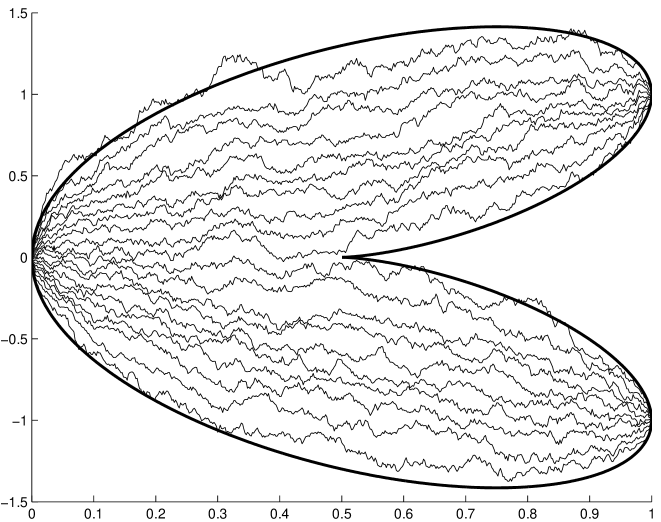
Figure 10. Non-intersecting Brownian paths that start at one point and end at two points. At any intermediate time the positions of the paths are distributed as the eigenvalues of a Gaussian random matrix ensemble with external source. As their number increases the paths fill out a region whose boundary has a cusp.

Consider $n$ independent Brownian motions (Brownian bridges) $x_{j}(t)$, $j=1,\dots,n$, on the line, starting at the origin at time $t=0$, half ending at $x=1$ and half at $x=-1$ at time $t=1$, and conditioned not to intersect for $t\in(0,1)$. Then at any time $t\in(0,1)$ the positions of $n$ non-intersecting Brownian bridges are distributed as the scaled eigenvalues,

$$\lambda_{j}=\frac{x_{j}}{\sqrt{t(1-t)}}\,,$$

of a Gaussian random matrix with the external source

$$a(t)=\sqrt{\frac{t}{1-t}}\,.$$

Fig.10 gives an illustration of the non-intersecting Brownian bridges. See also the paper [TW4] of Tracy and Widom on nonintersecting Brownian excursions.

In the Gaussian model the value $a=1$ is critical, and we will discuss its large $n$ asymptotics in the three cases:

1. $a>1$, two cuts,

2. $a<1$, one cut,

3. $a=1$, double scaling limit.

In the picture of the non-intersecting Brownian bridges this transforms to a critical time $t=\frac{1}{2}$, and there are two cuts for $t>\frac{1}{2}$, one cut for $t<\frac{1}{2}$, and the double scaling limit appears in a scaled neighborhood of $t=\frac{1}{2}$.

25. Gaussian model with external source. Main results

First we describe the limiting mean density of eigenvalues. The limiting mean density follows from earlier work of Pastur [Pas]. It is based on an analysis of the equation (Pastur equation)

$$\xi^{3}-z\xi^{2}+(1-a^{2})\xi+a^{2}z=0,$$ (25.1)

which yields an algebraic function $\xi(z)$ defined on a three-sheeted Riemann surface. The restrictions of $\xi(z)$ to the three sheets are denoted by $\xi_{j}(z)$, $j=1,2,3$. There are four real branch points if $a>1$ which determine two real intervals. The two intervals come together for $a=1$, and for $0<a<1$, there are two real branch points, and two purely imaginary branch points. Fig.11 depicts the structure of the Riemann surface $\xi(z)$ for $a>1$, $a=1$, and $a<1$.

Figure 11. The structure of the Riemann surface for the equation (25.1) for the values $a>1$ (left), $a=1$ (middle) and $a<1$ (right). In all cases the eigenvalues of $M$ accumulate on the interval(s) of the first sheet with a density given by (25.2).

In all cases we have that the limiting mean eigenvalue density $\rho(x)=\rho(x;a)$ is given by

$$\rho(x;a)=\frac{1}{\pi}{\operatorname{Im\,}}\xi_{1+}(x),\qquad x\in\mathbb{R},$$ (25.2)

where $\xi_{1+}(x)$ denotes the limiting value of $\xi_{1}(z)$ as $z\to x$ with ${\operatorname{Im\,}}z>0$. For $a=1$ the limiting mean eigenvalue density vanishes at $x=0$ and $\rho(x;a)\sim|x|^{1/3}$ as $x\to 0$.

We note that this behavior at the closing (or opening) of a gap is markedly different from the behavior that occurs in the usual unitary random matrix ensembles $Z_{n}^{-1}e^{-n{{\operatorname{Tr}\,}}V(M)}dM$ where a closing of the gap in the spectrum typically leads to a limiting mean eigenvalue density $\rho$ that satisfies $\rho(x)\sim(x-x^{*})^{2}$ as $x\to x^{*}$ if the gap closes at $x=x^{*}$. In that case the local eigenvalue correlations can be described in terms of $\psi$-functions associated with the Painlevé II equation, see above and [BI2, CK]. The phase transition for the model under consideration is different, and it cannot be realized in a unitary random matrix ensemble.

Theorem 25.1.

The limiting mean density of eigenvalues

$$\rho(x)=\lim_{n\to\infty}\frac{1}{n}K_{n}(x,x)$$ (25.3)

exists for every $a>0$. It satisfies

$$\rho(x)=\frac{1}{\pi}\left|\,{\operatorname{Im\,}}\xi(x)\right|,$$ (25.4)

where $\xi=\xi(x)$ is a solution of the cubic equation,

$$\xi^{3}-x\xi^{2}-(a^{2}-1)\xi+xa^{2}=0.$$ (25.5)

The support of $\rho$ consists of those $x\in\mathbb{R}$ for which (25.5) has a non-real solution.

1. For $0<a<1$, the support of $\rho$ consists of one interval $[-z_{1},z_{1}]$, and $\rho$ is real analytic and positive on $(-z_{1},z_{1})$, and it vanishes like a square root at the edge points $\pm z_{1}$, i.e., there exists a constant $\rho_{1}>0$ such that

   $$\rho(x)=\frac{\rho_{1}}{\pi}|x\mp z_{1}|^{1/2}(1+o(1))\qquad\mbox{as }x\to\pm z_{1},\,x\in(-z_{1},z_{1}).$$ (25.6)

2. For $a=1$, the support of $\rho$ consists of one interval $[-z_{1},z_{1}]$, and $\rho$ is real analytic and positive on $(-z_{1},0)\cup(0,z_{1})$, it vanishes like a square root at the edge points $\pm z_{1}$, and it vanishes like a third root at $0$, i.e., there exists a constant $c>0$ such that

   $$\rho(x)=c|x|^{1/3}\left(1+o(1)\right),\qquad\mbox{as }x\to 0.$$ (25.7)

3. For $a>1$, the support of $\rho$ consists of two disjoint intervals $[-z_{1},-z_{2}]\cup[z_{2},z_{1}]$ with $0<z_{2}<z_{1}$, $\rho$ is real analytic and positive on $(-z_{1},-z_{2})\cup(z_{2},z_{1})$, and it vanishes like a square root at the edge points $\pm z_{1}$, $\pm z_{2}$.

To describe the universality of local eigenvalue correlations in the large $n$ limit, we use a rescaled version of the kernel $K_{n}$:

$$\hat{K}_{n}(x,y)=e^{n(h(x)-h(y))}K_{n}(x,y)$$ (25.8)

for some function $h$. The rescaling is allowed because it does not affect the correlation functions $R_{m}$, which are expressed as determinants of the kernel. The function $h$ has the following form on $(-z_{1},-z_{2})\cup(z_{2},z_{1})$:

$$h(x)=-\frac{1}{4}x^{2}+{\operatorname{Re\,}}\int_{z_{1}}^{x}\xi_{1+}(s)ds,$$ (25.9)

where $\xi_{1}$ is a solution of the Pastur equation. The local eigenvalue correlations in the bulk of the spectrum in the large $n$ limit are described by the sine kernel. The bulk of the spectrum is the open interval $(-z_{1},z_{1})$ for $a<1$, and the union of the two open intervals, $(-z_{1},-z_{2})$ and $(z_{2},z_{1})$, for $a\geq 1$ ($z_{2}=0$ for $a=1$).

We have the following result:

Theorem 25.2.

For every $x_{0}$ in the bulk of the spectrum we have that

$$\lim_{n\to\infty} \frac{1}{n\rho(x_{0})}\hat{K}_{n}\left(x_{0}+\frac{u}{n\rho(x_{0})},x_{0}+\frac{v}{n\rho(x_{0})}\right)=\frac{\sin\pi(u-v)}{\pi(u-v)}.$$

At the edge of the spectrum the local eigenvalue correlations are described in the large $n$ limit by the Airy kernel:

Theorem 25.3.

For every $u,v\in{\mathbb{R}}$ we have

$$\lim_{n\to\infty} \frac{1}{(\rho_{1}n)^{2/3}}\hat{K}_{n}\left(z_{1}+\frac{u}{(\rho_{1}n)^{2/3}},z_{1}+\frac{v}{(\rho_{1}n)^{2/3}}\right)=\frac{{\operatorname{Ai}}(u){\operatorname{Ai}}^{\prime}(v)-{\operatorname{Ai}}^{\prime}(u){\operatorname{Ai}}(v)}{u-v}.$$

A similar limit holds near the edge point $-z_{1}$ and also near the edge points $\pm z_{2}$ if $a>1$.

As is usual in a critical case, there is a family of limiting kernels that arise when $a$ changes with $n$ and $a\to 1$ as $n\to\infty$ in a critical way. These kernels are constructed out of Pearcey integrals and therefore they are called Pearcey kernels. The Pearcey kernels were first described by Brézin and Hikami [BH4, BH5]. A detailed proof of the following result was recently given by Tracy and Widom [TW3].

Theorem 25.4.

We have for every fixed $b\in\mathbb{R}$,

$$\lim_{n\to\infty}\frac{1}{n^{3/4}}K_{n}\left(\frac{x}{n^{3/4}},\frac{y}{n^{3/4}};1+\frac{b}{2\sqrt{n}}\right)=K^{cusp}(x,y;b)$$ (25.10)

where $K^{cusp}$ is the Pearcey kernel

$$K^{cusp}(x,y;b)=\frac{p(x)q^{\prime\prime}(y)-p^{\prime}(x)q^{\prime}(y)+p^{\prime\prime}(x)q(y)-bp(x)q(y)}{x-y}$$ (25.11)

with

$$p(x)=\frac{1}{2\pi}\int_{-\infty}^{\infty}e^{-\frac{1}{4}s^{4}-\frac{b}{2}s^{2}+isx}ds\qquad\mbox{ and }\qquad q(y)=\frac{1}{2\pi}\int_{\Sigma}e^{\frac{1}{4}t^{4}+\frac{b}{2}t^{2}+ity}dt.$$ (25.12)

The contour $\Sigma$ consists of the four rays $\arg y=\pm\pi/4,\pm 3\pi/4$, with the orientation shown in Fig.12.

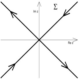
Figure 12. The contour $\Sigma$ that appears in the definition of $q(y)$.

The functions (25.12) are called Pearcey integrals [Pea]. They are solutions of the third order differential equations $p^{\prime\prime\prime}(x)=xp(x)+bp^{\prime}(x)$ and $q^{\prime\prime\prime}(y)=-yq(y)+bq^{\prime}(y)$, respectively.

Theorem 25.4 implies that local eigenvalue statistics of eigenvalues near $0$ are expressed in terms of the Pearcey kernel. For example we have the following corollary of Theorem 25.4.

Corollary 25.5.

The probability that a matrix of the ensemble (23.1), (23.43), with $a=1+bn^{-1/2}/2$ has no eigenvalues in the interval $[cn^{-3/4},dn^{-3/4}]$ converges, as $n\to\infty$, to the Fredholm determinant of the integral operator with kernel $K^{cusp}(x,y;b)$ acting on $L^{2}(c,d)$.

Similar expressions hold for the probability to have one, two, three, …, eigenvalues in an $O(n^{-3/4})$ neighborhood of $x=0$.

Tracy and Widom [TW3] and Adler and van Moerbeke [AvM3] gave differential equations for the gap probabilities associated with the Pearcey kernel and with the more general Pearcey process which arises from considering the non-intersecting Brownian motion model at several times near the critical time. See also [OR] where the Pearcey process appears in a combinatorial model on random partitions.

Brézin and Hikami and also Tracy and Widom used a double integral representation for the kernel in order to establish Theorem 25.4. We will describe the approach of [BK4], based on the Deift/Zhou steepest descent method for the Riemann-Hilbert problem for multiple Hermite polynomials. This method is less direct than the steepest descent method for integrals. However, an approach based on the Riemann-Hilbert problem may be applicable to more general situations, where an integral representation is not available. This is the case, for example, for the general (non-Gaussian) unitary random matrix ensemble with external source, (23.1), with a general potential $V$.

The proof of the theorems above is based on the construction of a parametrix of the RHP, and we will describe this construction for the cases $a>1$, $a<1$, and $a=1$.

26. Construction of a parametrix in the case $a>1$

Consider the Riemann surface given by equation (25.1) for $a>1$, see the left surface on Fig.11. There are three roots to this equation, which behave at infinity as

$$\xi_{1}(z) =z-\frac{1}{z}+O\left(\frac{1}{z^{3}}\right),\qquad\xi_{2,3}(z) =\pm a+\frac{1}{2z}+O\left(\frac{1}{z^{2}}\right).$$ (26.1)

We need the integrals of the $\xi$-functions,

$$\lambda_{k}(z)=\int^{z}\xi_{k}(s)ds,\qquad k=1,2,3,$$ (26.2)

which we take so that $\lambda_{1}$ and $\lambda_{2}$ are analytic on $\mathbb{C}\setminus(-\infty,z_{1}]$ and $\lambda_{3}$ is analytic on $\mathbb{C}\setminus(-\infty,-z_{2}]$. Then, as $z\to\infty$,

$$\lambda_{1}(z) =\frac{z^{2}}{2}-\ln z+l_{1}+O\left(\frac{1}{z^{2}}\right),\qquad\lambda_{2,3}(z) =\pm az+\frac{1}{2}\ln z+l_{2,3}+O\left(\frac{1}{z}\right),$$ (26.3)

where $l_{1}$, $l_{2}$, $l_{3}$ are some constants, which we choose as follows. We choose $l_{1}$ and $l_{2}$ such that

$$\lambda_{1}(z_{1})=\lambda_{2}(z_{1})=0,$$ (26.4)

and then $l_{3}$ such that

$$\lambda_{3}(-z_{2})=\lambda_{1+}(-z_{2})=\lambda_{1-}(-z_{2})-\pi i.$$ (26.5)

First Transformation of the RH Problem. Using the functions $\lambda_{j}$ and the constants $l_{j}$, $j=1,2,3$, we define

$$T(z) ={\operatorname{diag}}\left(e^{-nl_{1}},e^{-nl_{2}},e^{-nl_{3}}\right)Y(z){\operatorname{diag}}\left(e^{n(\lambda_{1}(z)-\frac{1}{2}z^{2})},e^{n(\lambda_{2}(z)-az)},e^{n(\lambda_{3}(z)+az)}\right).$$ (26.6)

Then $T_{+}(x)=T_{-}(x)j_{T}(x)$, $x\in\mathbb{R}$, where for $x\in[z_{2},z_{1}]$,

$$j_{T} =\begin{pmatrix}e^{n(\lambda_{1}-\lambda_{2})_{+}}&1&e^{n(\lambda_{3}-\lambda_{1-})}\\ 0&e^{n(\lambda_{1}-\lambda_{2})_{-}}&0\\ 0&0&1\end{pmatrix}$$ (26.7)

and for $x\in[-z_{1},-z_{2}]$,

$$j_{T} =\begin{pmatrix}e^{n(\lambda_{1}-\lambda_{3})_{+}}&e^{n(\lambda_{2+}-\lambda_{1-})}&1\\ 0&1&0\\ 0&0&e^{n(\lambda_{1}-\lambda_{3})_{-}}\end{pmatrix}.$$ (26.8)

Second transformation of the RH Problem: opening of lenses. The lens structure is shown on Fig.13.

Figure 13. The lenses for $a>1$.

Set in the right lens,

$$S(z)=\left\{\begin{aligned} {}&T(z)\begin{pmatrix}1&0&0\\ -e^{n(\lambda_{1}(z)-\lambda_{2}(z))}&1&-e^{n(\lambda_{3}(z)-\lambda_{2}(z))}\\ 0&0&1\end{pmatrix}\\ {}&\;\text{\rm in the upper lens region},\\ {}&T(z)\begin{pmatrix}1&0&0\\ e^{n(\lambda_{1}(z)-\lambda_{2}(z))}&1&-e^{n(\lambda_{3}(z)-\lambda_{2}(z))}\\ 0&0&1\end{pmatrix}\\ {}&\;\text{\rm in the lower lens region},\end{aligned}\right.$$ (26.9)

and, respectively, in the left lens,

$$S(z)=\left\{\begin{aligned} {}&T(z)\begin{pmatrix}1&0&0\\ 0&1&0\\ -e^{n(\lambda_{1}(z)-\lambda_{3}(z))}&-e^{n(\lambda_{2}(z)-\lambda_{3}(z))}&1\end{pmatrix}\\ {}&\;\text{\rm in the upper lens region},\\ {}&T(z)\begin{pmatrix}1&0&0\\ 0&1&0\\ e^{n(\lambda_{1}(z)-\lambda_{3}(z)))}&-e^{n(\lambda_{2}(z)-\lambda_{3}(z))}&1\end{pmatrix}\\ {}&\;\text{\rm in the lower lens region}.\end{aligned}\right.$$ (26.10)

Then

$$S_{+}(x) =S_{-}(x)j_{S}(x);\qquad j_{S}(x) =\begin{pmatrix}0&1&0\\ -1&0&0\\ 0&0&1\end{pmatrix},\quad x\in[z_{2},z_{1}],$$ (26.11)

and

$$S_{+}(x) =S_{-}(x)j_{S}(x);\qquad j_{S}(x) =\begin{pmatrix}0&0&1\\ 0&1&0\\ -1&0&0\end{pmatrix},\quad x\in[-z_{1},-z_{2}].$$ (26.12)

In addition, $S$ has jumps on the boundary of the lenses, which are exponentially small away of the points $\pm z_{1,2}$. The RH problem for $S$ is approximated by the model RH problem.

Model RH problem

• $M$ is analytic on ${\mathbb{C}}\setminus([-z_{1},-z_{2}]\cup[z_{2},z_{1}])$,

• $$M_{+}(x)=M_{-}(x)j_{S}(x),\quad x\in(-z_{1},-z_{2})\cup(z_{2},z_{1}),$$ (26.13)

• as $z\to\infty$,

  $$M(z)=I+O\left(\frac{1}{z}\right),$$ (26.14)

where the jump matrix is

$$j_{S}(x)=\left\{\begin{aligned} {}&\begin{pmatrix}0&1&0\\ -1&0&0\\ 0&0&1\end{pmatrix},\quad x\in(z_{2},z_{1})\\ {}&\begin{pmatrix}0&0&1\\ 0&1&0\\ -1&0&0\end{pmatrix},\quad x\in(-z_{1},-z_{2}).\end{aligned}\right.$$ (26.15)

Solution to the model RH problem has the form:

$$M(z)=A(z)B(z)C(z),$$ (26.16)

where

$$A(z)=\textrm{diag}\left(1,-\frac{i}{\sqrt{2}},-\frac{i}{\sqrt{2}}\right),\qquad B(z)=\begin{pmatrix}\xi_{1}^{2}(z)-a^{2}&\xi_{2}^{2}(z)-a^{2}&\xi_{3}^{2}(z)-a^{2}\\ \xi_{1}(z)+a&\xi_{2}(z)+a&\xi_{3}(z)+a\\ \xi_{1}(z)-a&\xi_{2}(z)-a&\xi_{3}(z)-a\end{pmatrix}$$ (26.17)

and

$$C(z)=\textrm{diag}\left(\frac{1}{\sqrt{Q(\xi_{1}(z))}},\frac{1}{\sqrt{Q(\xi_{2}(z))}},\frac{1}{\sqrt{Q(\xi_{3}(z))}}\right)$$ (26.18)

where

$$Q(z)=z^{4}-(1+2a^{2})z^{2}+(a^{2}-1)a^{2}.$$ (26.19)

Parametrix at edge points. We consider small disks $D(\pm z_{j},r)$ with radius $r>0$ and centered at the edge points, and look for a local parametrix $P$ defined on the union of the four disks such that

• $P$ is analytic on $D(\pm z_{j},r)\setminus({\mathbb{R}}\cup\Gamma)$,

• $$P_{+}(z)=P_{-}(z)j_{S}(z),\quad z\in({\mathbb{R}}\cup\Gamma)\cap D(\pm z_{j},r),$$ (26.20)

• as $n\to\infty$,

  $$P(z)=\left(I+O\left(\frac{1}{n}\right)\right)M(z)\quad\text{\rm uniformly for $z\in\partial D(\pm z_{j},r)$}.$$ (26.21)

Figure 14. Partition of a neighborhood of the edge point.

We consider here the edge point $z_{1}$ in detail. We note that as $z\to z_{1}$,

$$\lambda_{1}(z) =q(z-z_{1})+\frac{2\rho_{1}}{3}(z-z_{1})^{3/2}+O(z-z_{1})^{2}$$ (26.22)

$$\lambda_{2}(z) =q(z-z_{1})-\frac{2\rho_{1}}{3}(z-z_{1})^{3/2}+O(z-z_{1})^{2}$$

so that

$$\lambda_{1}(z)-\lambda_{2}(z)=\frac{4\rho_{1}}{3}(z-z_{1})^{3/2}+O(z-z_{1})^{5/2}$$ (26.23)

as $z\to z_{1}$. Then it follows that

$$\beta(z)=\left[\frac{3}{4}(\lambda_{1}(z)-\lambda_{2}(z))\right]^{2/3}$$ (26.24)

is analytic at $z_{1}$, real-valued on the real axis near $z_{1}$ and $\beta^{\prime}(z_{1})=\rho_{1}^{2/3}>0$. So $\beta$ is a conformal map from $D(z_{1},r)$ to a convex neighborhood of the origin, if $r$ is sufficiently small (which we assume to be the case). We take $\Gamma$ near $z_{1}$ such that

$$\beta(\Gamma\cap D(z_{1},r))\subset\{z\mid\arg(z)=\pm 2\pi/3\}.$$

Then $\Gamma$ and ${\mathbb{R}}$ divide the disk $D(z_{1},r)$ into four regions numbered I, II, III, and IV, such that $0<\arg\beta(z)<2\pi/3$, $2\pi/3<\arg\beta(z)<\pi$, $-\pi<\arg\beta(z)<-2\pi/3$, and $-2\pi/3<\arg\beta(z)<0$ for $z$ in regions I, II, III, and IV, respectively, see Fig.14.

Recall that the jumps $j_{S}$ near $z_{1}$ are given as

$$j_{S} =\begin{pmatrix}0&1&0\\ -1&0&0\\ 0&0&1\end{pmatrix}\qquad\text{\rm on }[z_{1}-r,z_{1})$$ (26.25)

$$j_{S} =\begin{pmatrix}1&0&0\\ e^{n(\lambda_{1}-\lambda_{2})}&1&e^{n(\lambda_{3}-\lambda_{2})}\\ 0&0&1\end{pmatrix}\;\text{\rm on the upper boundary of the lens in $D(z_{1},r)$ }$$

$$j_{S} =\begin{pmatrix}1&0&0\\ e^{n(\lambda_{1}-\lambda_{2})}&1&-e^{n(\lambda_{3}-\lambda_{2})}\\ 0&0&1\end{pmatrix}\;\text{\rm on the lower boundary of the lens in $D(z_{1},r)$}$$

$$j_{S} =\begin{pmatrix}1&e^{n(\lambda_{2}-\lambda_{1})}&e^{n(\lambda_{3}-\lambda_{1})}\\ 0&1&0\\ 0&0&1\end{pmatrix}\qquad\text{\rm on }(z_{1},z_{1}+r].$$

We write

$$\tilde{P}=\left\{\begin{array}[]{ll}P\begin{pmatrix}1&0&0\\ 0&1&-e^{n(\lambda_{3}-\lambda_{2})}\\ 0&0&1\end{pmatrix}&\text{\rm in regions I and IV}\\ P&\text{\rm in regions II and III.}\end{array}\right.$$ (26.26)

Then the jumps for $\tilde{P}$ are $\tilde{P}_{+}=\tilde{P}_{-}j_{\tilde{P}}$ where

$$j_{\tilde{P}} =\begin{pmatrix}0&1&0\\ -1&0&0\\ 0&0&1\end{pmatrix}\qquad\text{\rm on }[z_{1}-r,z_{1})$$ (26.27)

$$j_{\tilde{P}} =\begin{pmatrix}1&0&0\\ e^{n(\lambda_{1}-\lambda_{2})}&1&0\\ 0&0&1\end{pmatrix}\;\text{\rm on the upper side of the lens in }D(z_{1},r)$$

$$j_{\tilde{P}} =\begin{pmatrix}1&0&0\\ e^{n(\lambda_{1}-\lambda_{2})}&1&0\\ 0&0&1\end{pmatrix}\;\text{\rm on the lower side of the lens in }D(z_{1},r)$$

$$j_{\tilde{P}} =\begin{pmatrix}1&e^{n(\lambda_{2}-\lambda_{1})}&0\\ 0&1&0\\ 0&0&1\end{pmatrix}\qquad\text{\rm on }(z_{1},z_{1}+r].$$

We also need the matching condition

$$\tilde{P}(z)=\left(I+O\left(\frac{1}{n}\right)\right)M(z)\quad\text{\rm uniformly for $z\in\partial D(z_{1},r)$}.$$ (26.28)

The RH problem for $\tilde{P}$ is essentially a $2\times 2$ problem, since the jumps (26.27) are non-trivial only in the upper $2\times 2$ block. A solution can be constructed in a standard way out of Airy functions. The Airy function ${\operatorname{Ai}}(z)$ solves the equation $y^{\prime\prime}=zy$ and for any $\varepsilon>0$, in the sector $\pi+\varepsilon\leq\arg z\leq\pi-\varepsilon$, it has the asymptotics as $z\to\infty$,

$${\operatorname{Ai}}(z)=\frac{1}{2\sqrt{\pi}z^{1/4}}e^{-\frac{2}{3}z^{3/2}}\left(1+O(z^{-3/2})\right).$$ (26.29)

The functions ${\operatorname{Ai}}(\omega z)$, ${\operatorname{Ai}}(\omega^{2}z)$, where $\omega=e^{\frac{2\pi i}{3}}$, also solve the equation $y^{\prime\prime}=zy$, and we have the linear relation,

$${\operatorname{Ai}}(z)+\omega{\operatorname{Ai}}(\omega z)+\omega^{2}{\operatorname{Ai}}(\omega^{2}z)=0.$$ (26.30)

Write

$$y_{0}(z)={\operatorname{Ai}}(z),\quad y_{1}(z)=\omega{\operatorname{Ai}}(\omega z),\quad y_{2}(z)=\omega^{2}{\operatorname{Ai}}(\omega^{2}z),$$ (26.31)

and we use these functions to define

$$\Phi(z)=\left\{\begin{aligned} {}&\begin{pmatrix}y_{0}(z)&-y_{2}(z)&0\\ y_{0}^{\prime}(z)&-y_{2}^{\prime}(z)&0\\ 0&0&1\end{pmatrix},\quad\mbox{for $0<\arg z<2\pi/3$},\\ {}&\begin{pmatrix}-y_{1}(z)&-y_{2}(z)&0\\ -y_{1}^{\prime}(z)&-y_{2}^{\prime}(z)&0\\ 0&0&1\end{pmatrix},\quad\mbox{for $2\pi/3<\arg z<\pi$},\\ {}&\begin{pmatrix}-y_{2}(z)&y_{1}(z)&0\\ -y_{2}^{\prime}(z)&y_{1}^{\prime}(z)&0\\ 0&0&1\end{pmatrix},\quad\mbox{for $-\pi<\arg z<-2\pi/3$},\\ {}&\begin{pmatrix}y_{0}(z)&y_{1}(z)&0\\ y_{0}^{\prime}(z)&y_{1}^{\prime}(z)&0\\ 0&0&1\end{pmatrix},\quad\mbox{for $-2\pi/3<\arg z<0$}.\end{aligned}\right.$$ (26.32)

Then

$$\tilde{P}(z)=E_{n}(z)\Phi(n^{2/3}\beta(z)){\operatorname{diag}}\left(e^{\frac{1}{2}n(\lambda_{1}(z)-\lambda_{2}(z))},e^{-\frac{1}{2}n(\lambda_{1}(z)-\lambda_{2}(z))},1\right)$$ (26.33)

where $E_{n}$ is an analytic prefactor that takes care of the matching condition (26.28). Explicitly, $E_{n}$ is given by

$$E_{n}=\sqrt{\pi}M\begin{pmatrix}1&-1&0\\ -i&-i&0\\ 0&0&1\end{pmatrix}\begin{pmatrix}n^{1/6}\beta^{1/4}&0&0\\ 0&n^{-1/6}\beta^{-1/4}&0\\ 0&0&1\end{pmatrix}.$$ (26.34)

A similar construction works for a parametrix $P$ around the other edge points.

Third transformation. In the third and final transformation we put

$$R(z) =S(z)M(z)^{-1}\quad\text{\rm for $z$ outside the disks $D(\pm z_{j},r)$, $j=1,2$}$$ (26.35)

$$R(z) =S(z)P(z)^{-1}\quad\text{\rm for $z$ inside the disks.}$$

Then $R$ is analytic on ${\mathbb{C}}\setminus\Gamma_{R}$, where $\Gamma_{R}$ consists of the four circles $\partial D(\pm z_{j},r)$, $j=1,2$, the parts of $\Gamma$ outside the four disks, and the real intervals $(-\infty,-z_{1}-r)$, $(-z_{2}+r,z_{2}-r)$, $(z_{1}+r,\infty)$, see Fig.15.

Figure 15. The contour $\Gamma_{R}$ for $R$.

There are jump relations

$$R_{+}=R_{-}j_{R}$$ (26.36)

where

$$j_{R} =MP^{-1}\quad\text{\rm on the circles, oriented counterclockwise}$$ (26.37)

$$j_{R} =Mj_{S}M^{-1}\quad\text{\rm on the remaining parts of $\Gamma_{R}$.}$$

We have that $j_{R}=I+O(1/n)$ uniformly on the circles, and $j_{R}=I+O(e^{-cn})$ for some $c>0$ as $n\to\infty$, uniformly on the remaining parts of $\Gamma_{R}$. So we can conclude

$$j_{R}(z)=I+O\left(\frac{1}{n}\right)\quad\text{\rm as $n\to\infty$, uniformly on $\Gamma_{R}$.}$$ (26.38)

As $z\to\infty$, we have

$$R(z)=I+O(1/z).$$ (26.39)

From (26.36), (26.38), (26.39) and the fact that we can deform the contours in any desired direction, it follows that

$$R(z)=I+O\left(\frac{1}{n(|z|+1)}\right)\quad\mbox{as }n\to\infty.$$ (26.40)

uniformly for $z\in{\mathbb{C}}\setminus\Gamma_{R}$, see [Dei, DKMVZ, DKMVZ2, Kui].

27. Construction of a parametrix in the case $a<1$

27.1. $\lambda$-functions

Consider the Riemann surface given by equation (25.1) for $a<1$, see the right surface on Fig.11. There are three roots to this equation, which behave at infinity as in (26.1). We need the integrals of the $\xi$-functions, which we define as

$$\lambda_{1}(z) =\int_{z_{1}}^{z}\xi_{1}(s)ds,$$ (27.1)

$$\lambda_{2}(z) =\int_{z_{1}}^{z}\xi_{2}(s)ds,$$

$$\lambda_{3}(z) =\int_{-z_{1+}}^{z}\xi_{3}(s)ds+\lambda_{1-}(-z_{1}),$$

The path of integration for $\lambda_{3}$ lies in $\mathbb{C}\setminus((-\infty,0]\cup[-iz_{2},iz_{2}])$, and it starts at the point $-z_{1}$ on the upper side of the cut. All three $\lambda$-functions are defined on their respective sheets of the Riemann surface with an additional cut along the negative real axis. Thus $\lambda_{1},\lambda_{2},\lambda_{3}$ are defined and analytic on $\mathbb{C}\setminus(-\infty,z_{1}]$, $\mathbb{C}\setminus((-\infty,z_{1}]\cup[-iz_{2},iz_{2}])$, and $\mathbb{C}\setminus((-\infty,0]\cup[-iz_{2},iz_{2}])$, respectively. Their behavior at infinity is

$$\lambda_{1}(z) =\frac{1}{2}z^{2}-\log z+\ell_{1}+O(1/z)$$ (27.2)

$$\lambda_{2}(z) =az+\frac{1}{2}\log z+\ell_{2}+O(1/z)$$

$$\lambda_{3}(z) =-az+\frac{1}{2}\log z+\ell_{3}+O(1/z)$$

for certain constants $\ell_{j}$, $j=1,2,3$. The $\lambda_{j}$’s satisfy the following jump relations

$$\begin{array}[]{ll}\lambda_{1\mp}=\lambda_{2\pm}&\textrm{ on }(0,z_{1}),\\ \lambda_{1-}=\lambda_{3+}&\textrm{ on }(-z_{1},0),\\ \lambda_{1+}=\lambda_{3-}-\pi i&\textrm{ on }(-z_{1},0),\\ \lambda_{2\mp}=\lambda_{3\pm}&\textrm{ on }(0,iz_{2}),\\ \lambda_{2\mp}=\lambda_{3\pm}-\pi i&\textrm{ on }(-iz_{2},0),\\ \lambda_{1+}=\lambda_{1-}-2\pi i&\textrm{ on }(-\infty,-z_{1}),\\ \lambda_{2+}=\lambda_{2-}+\pi i&\textrm{ on }(-\infty,0),\\ \lambda_{3+}=\lambda_{3-}+\pi i&\textrm{ on }(-\infty,-z_{1}),\end{array}$$ (27.3)

where the segment $(-iz_{2},iz_{2})$ is oriented upwards.

27.2. First transformation $Y\mapsto U$

We define for $z\in\mathbb{C}\setminus(\mathbb{R}\cup[-iz_{2},iz_{2}])$,

$$U(z)={\operatorname{diag}}(e^{-n\ell_{1}},e^{-n\ell_{2}},e^{-n\ell_{3}})Y(z){\operatorname{diag}}(e^{n(\lambda_{1}(z)-\frac{1}{2}z^{2})},e^{n(\lambda_{2}(z)-az)},e^{n(\lambda_{3}(z)+az)}).$$ (27.4)

This coincides with the first transformation for $a>1$. Then $U$ solves the following RH problem.

• $U:\mathbb{C}\setminus(\mathbb{R}\cup[-iz_{2},iz_{2}])\to\mathbb{C}^{3\times 3}$ is analytic.

• $U$ satisfies the jumps

  $$U_{+}=U_{-}\begin{pmatrix}e^{n(\lambda_{1+}-\lambda_{1-})}&e^{n(\lambda_{2+}-\lambda_{1-})}&e^{n(\lambda_{3+}-\lambda_{1-})}\\ 0&e^{n(\lambda_{2+}-\lambda_{2-})}&0\\ 0&0&e^{n(\lambda_{3+}-\lambda_{3-})}\end{pmatrix}\qquad\textrm{ on }\mathbb{R},$$ (27.5)

  and

  $$U_{+}=U_{-}\begin{pmatrix}1&0&0\\ 0&e^{n(\lambda_{2+}-\lambda_{2-})}&0\\ 0&0&e^{n(\lambda_{3+}-\lambda_{3-})}\end{pmatrix}\qquad\textrm{on }[-iz_{2},iz_{2}].$$ (27.6)

• $U(z)=I+O(1/z)$ as $z\to\infty$.

27.3. Second transformation $U\mapsto T$: global opening of a lens on $[-iz_{2},iz_{2}]$

The second transformation is the opening of a lens on the interval $[-iz_{2},iz_{2}]$. We consider a contour $\Sigma$, which goes first from $(-iz_{2})$ to $iz_{2}$ around the point $z_{1}$, and then from $iz_{2}$ to $(-iz_{2})$ around the point $-z_{1}$, see Fig.16, and such that for $z\in\Sigma$,

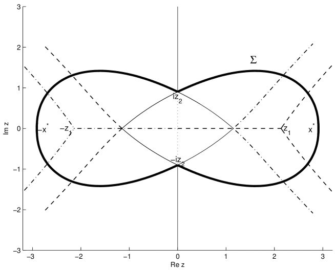
Figure 16. Contour $\Sigma$ which is such that ${\operatorname{Re\,}}\lambda_{2}<{\operatorname{Re\,}}\lambda_{3}$ on the part of $\Sigma$ in the left half-plane and ${\operatorname{Re\,}}\lambda_{2}>{\operatorname{Re\,}}\lambda_{3}$ on the part of $\Sigma$ in the right half-plane.

$$\pm\left({\operatorname{Re\,}}\lambda_{2}(z)-{\operatorname{Re\,}}\lambda_{3}(z)\right)>0,\quad\pm{\operatorname{Re\,}}z>0.$$ (27.7)

Observe that inside the curvilinear quadrilateral marked by a solid line on Fig.16, $\pm\left({\operatorname{Re\,}}\lambda_{2}(z)-{\operatorname{Re\,}}\lambda_{3}(z)\right)<0$, hence the contour $\Sigma$ has to stay outside of this quadrilateral. We set $T=U$ outside $\Sigma$, and inside $\Sigma$ we set

$$T =U\begin{pmatrix}1&0&0\\ 0&1&0\\ 0&-e^{n(\lambda_{2}-\lambda_{3})}&1\end{pmatrix}\qquad\textrm{for }{\operatorname{Re\,}}z<0\textrm{ inside }\Sigma,$$ (27.8)

$$T =U\begin{pmatrix}1&0&0\\ 0&1&-e^{n(\lambda_{3}-\lambda_{2})}\\ 0&0&1\end{pmatrix}\qquad\textrm{for }{\operatorname{Re\,}}z>0\textrm{ inside }\Sigma.$$

27.4. Third transformation $T\mapsto S$: opening of a lens on $[-z_{1},z_{1}]$

We open a lens on $[-z_{1},z_{1}]$, inside of $\Sigma$, see Fig.17, and we define $S=T$ outside of the lens and

$$S =T\begin{pmatrix}1&0&0\\ 0&1&0\\ -e^{n(\lambda_{1}-\lambda_{3})}&0&1\end{pmatrix}\qquad\textrm{in upper part of the lens in left half-plane,}$$ (27.9)

$$S =T\begin{pmatrix}1&0&0\\ 0&1&0\\ e^{n(\lambda_{1}-\lambda_{3})}&0&1\end{pmatrix}\qquad\textrm{in lower part of the lens in left half-plane,}$$

$$S =T\begin{pmatrix}1&0&0\\ -e^{n(\lambda_{1}-\lambda_{2})}&1&0\\ 0&0&1\end{pmatrix}\qquad\textrm{in upper part of the lens in right half-plane,}$$

$$S =T\begin{pmatrix}1&0&0\\ e^{n(\lambda_{1}-\lambda_{2})}&1&0\\ 0&0&1\end{pmatrix}\qquad\textrm{in lower part of the lens in right half-plane.}$$

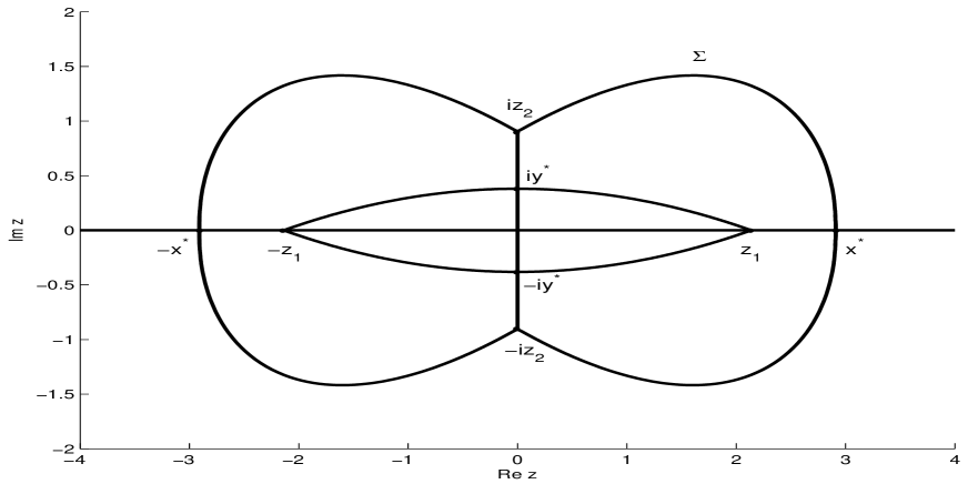
Figure 17. Opening of a lens around $[-z_{1},z_{1}]$.

Then $S$ satisfies the following RH problem:

• $S$ is analytic outside the real line, the vertical segment $[-iz_{2},iz_{2}]$, the curve $\Sigma$, and the upper and lower lips of the lens around $[-z_{1},z_{1}]$.

• $S$ satisfies the following jumps on the real line

  $$S_{+} =S_{-}\begin{pmatrix}1&e^{n(\lambda_{2+}-\lambda_{1-})}&e^{n(\lambda_{3+}-\lambda_{1-})}\\ 0&1&0\\ 0&0&1\end{pmatrix}\qquad\textrm{on }(-\infty,-x^{*}]$$ (27.10)

  $$S_{+} =S_{-}\begin{pmatrix}1&0&e^{n(\lambda_{3+}-\lambda_{1-})}\\ 0&1&0\\ 0&0&1\end{pmatrix}\qquad\textrm{on }(-x^{*},-z_{1}]$$ (27.11)

  $$S_{+} =S_{-}\begin{pmatrix}0&0&1\\ 0&1&0\\ -1&0&0\end{pmatrix}\qquad\textrm{on }(-z_{1},0)$$ (27.12)

  $$S_{+} =S_{-}\begin{pmatrix}0&1&0\\ -1&0&0\\ 0&0&1\end{pmatrix}\qquad\textrm{on }(0,z_{1})$$ (27.13)

  $$S_{+} =S_{-}\begin{pmatrix}1&e^{n(\lambda_{2}-\lambda_{1})}&0\\ 0&1&0\\ 0&0&1\end{pmatrix}\qquad\textrm{on }[z_{1},x^{*})$$ (27.14)

  $$S_{+} =S_{-}\begin{pmatrix}1&e^{n(\lambda_{2}-\lambda_{1})}&e^{n(\lambda_{3}-\lambda_{1})}\\ 0&1&0\\ 0&0&1\end{pmatrix}\qquad\textrm{on }[x^{*},\infty).$$ (27.15)

  $S$ has the following jumps on the segment $[-iz_{2},iz_{2}]$,

  $$S_{+} =S_{-}\begin{pmatrix}1&0&0\\ 0&0&1\\ 0&-1&e^{n(\lambda_{3+}-\lambda_{3-})}\end{pmatrix}\qquad\textrm{on }(-iz_{2},-iy^{*})$$ (27.16)

  $$S_{+} =S_{-}\begin{pmatrix}1&0&0\\ 0&0&1\\ e^{n(\lambda_{1}-\lambda_{3-})}&-1&e^{n(\lambda_{3+}-\lambda_{3-})}\end{pmatrix}\qquad\textrm{on }(-iy^{*},0)$$ (27.17)

  $$S_{+} =S_{-}\begin{pmatrix}1&0&0\\ 0&0&1\\ -e^{n(\lambda_{1}-\lambda_{3-})}&-1&e^{n(\lambda_{3+}-\lambda_{3-})}\end{pmatrix}\qquad\textrm{on }(0,iy^{*})$$ (27.18)

  $$S_{+} =S_{-}\begin{pmatrix}1&0&0\\ 0&0&1\\ 0&-1&e^{n(\lambda_{3+}-\lambda_{3-})}\end{pmatrix}\qquad\textrm{on }(iy^{*},iz_{2}).$$ (27.19)

  The jumps on $\Sigma$ are

  $$S_{+} =S_{-}\begin{pmatrix}1&0&0\\ 0&1&0\\ 0&e^{n(\lambda_{2}-\lambda_{3})}&1\end{pmatrix}\qquad\textrm{on }\{z\in\Sigma\mid{\operatorname{Re\,}}z<0\}$$ (27.20)

  $$S_{+} =S_{-}\begin{pmatrix}1&0&0\\ 0&1&e^{n(\lambda_{3}-\lambda_{2})}\\ 0&0&1\end{pmatrix}\qquad\textrm{on }\{z\in\Sigma\mid{\operatorname{Re\,}}z>0\}.$$ (27.21)

  Finally, on the upper and lower lips of the lens, we find jumps

  $$S_{+} =S_{-}\begin{pmatrix}1&0&0\\ 0&1&0\\ e^{n(\lambda_{1}-\lambda_{3})}&0&1\end{pmatrix}\qquad\textrm{on the lips of the lens in the left half-plane}$$ (27.22)

  $$S_{+} =S_{-}\begin{pmatrix}1&0&0\\ e^{n(\lambda_{1}-\lambda_{2})}&1&0\\ 0&0&1\end{pmatrix}\qquad\textrm{on the lips of the lens in the right half-plane.}$$ (27.23)

• $S(z)=I+O(1/z)$ as $z\to\infty$.

As $n\to\infty$, the jump matrices have limits. Most of the limits are the identity matrix, except for the jumps on $(-z_{1},z_{1})$, see (27.12) and (27.13), and on $(-iz_{2},iz_{2})$, see (27.16)–(27.19). The limiting model RH problem can be solved explicitly. The solution is similar to the case $a>1$, and it is given by formulas (26.16)-(26.19), with cuts of the function $\sqrt{P(z)}$ on the intervals $[-z_{1},z_{1}]$ and $[-iz_{2},iz_{2}]$.

27.5. Local parametrix at the branch points for $a<1$.

Near the branch points the model solution $M$ will not be a good approximation to $S$. We need a local analysis near each of the branch points. In a small circle around each of the branch points, the parametrix $P$ should have the same jumps as $S$, and on the boundary of the circle $P$ should match with $M$ in the sense that

$$P(z)=M(z)\left(I+O(1/n)\right)$$ (27.24)

uniformly for $z$ on the boundary of the circle.

The construction of $P$ near the real branch points $\pm z_{1}$ makes use of Airy functions and it is the same as the one given above for the case $a>1$. The parametrix near the imaginary branch points $\pm iz_{2}$ is also constructed with Airy functions. We give the construction near $iz_{2}$. There are three contours, parts of $\Sigma$, meeting at $iz_{2}$: left, right and vertical, see Fig.17. We want an analytic $P$ in a neigborhood of $iz_{2}$ with jumps

$$P_{+} =P_{-}\begin{pmatrix}1&0&0\\ 0&1&0\\ 0&e^{n(\lambda_{2}-\lambda_{3})}&1\end{pmatrix}\qquad\textrm{on left contour}$$ (27.25)

$$P_{+} =P_{-}\begin{pmatrix}1&0&0\\ 0&1&e^{n(\lambda_{3}-\lambda_{2})}\\ 0&0&1\end{pmatrix}\qquad\textrm{on right contour}$$

$$P_{+} =P_{-}\begin{pmatrix}1&0&0\\ 0&0&1\\ 0&-1&e^{n(\lambda_{3+}-\lambda_{3-})}\end{pmatrix}\qquad\textrm{on vertical part.}$$

In addition we need the matching condition (27.24). Except for the matching condition (27.24), the problem is a $2\times 2$ problem. We define

$$f(z)=\left[\frac{3}{4}(\lambda_{2}-\lambda_{3})(z)\right]^{2/3}$$ (27.26)

such that

$$\arg f(z)=\pi/3,\qquad\textrm{ for }z=iy,\,y>z_{2}.$$

Then $s=f(z)$ is a conformal map, which maps $[0,iz_{2}]$ into the ray $\arg s=-\frac{2\pi}{3}$, and which maps the parts of $\Sigma$ near $iz_{2}$ in the right and left half-planes into the rays $\arg s=0$ and $\arg s=\frac{2\pi}{3}$, respectively. The local parametrix has the form,

$$P(z)=E(z)\Phi\left(n^{2/3}f(z)\right)\begin{pmatrix}1&0&0\\ 0&e^{\frac{1}{2}n(\lambda_{2}-\lambda_{3})}&0\\ 0&0&e^{-\frac{1}{2}n(\lambda_{2}-\lambda_{3})}\end{pmatrix}$$ (27.27)

where $E$ is analytic. The model matrix-valued function $\Phi$ is defined as

$$\Phi =\begin{pmatrix}1&0&0\\ 0&y_{0}&-y_{2}\\ 0&y_{0}^{\prime}&-y_{2}^{\prime}\end{pmatrix}\qquad\textrm{for }0<\arg s<2\pi/3,$$ (27.28)

$$\Phi =\begin{pmatrix}1&0&0\\ 0&y_{0}&y_{1}\\ 0&y_{0}^{\prime}&y_{1}^{\prime}\end{pmatrix}\qquad\textrm{for }-2\pi/3<\arg s<0,$$

$$\Phi =\begin{pmatrix}1&0&0\\ 0&-y_{1}&-y_{2}\\ 0&-y_{1}^{\prime}&-y_{2}^{\prime}\end{pmatrix}\qquad\textrm{for }2\pi/3<\arg s<4\pi/3,$$

where $y_{0}(s)={\operatorname{Ai}}(s)$, $y_{1}(s)=\omega{\operatorname{Ai}}(\omega s)$, $y_{2}(s)=\omega^{2}{\operatorname{Ai}}(\omega^{2}s)$ with $\omega=2\pi/3$ and ${\operatorname{Ai}}$ the standard Airy function. In order to achieve the matching (27.24) we define the prefactor $E$ as

$$E=ML^{-1}$$ (27.29)

with

$$L=\frac{1}{2\sqrt{\pi}}\begin{pmatrix}1&0&0\\ 0&n^{-1/6}f^{-1/4}&0\\ 0&0&n^{1/6}f^{1/4}\end{pmatrix}\begin{pmatrix}1&0&0\\ 0&1&i\\ 0&-1&i\end{pmatrix}$$ (27.30)

where $f^{1/4}$ has a branch cut along the vertical segment $[0,iz_{2}]$ and it is real and positive where $f$ is real and positive. The matching condition (27.24) now follows from the asymptotics of the Airy function and its derivative.

A similar construction gives the parametrix in the neighborhood of $-iz_{2}$.

27.6. Fourth transformation $S\mapsto R$

Having constructed $N$ and $P$, we define the final transformation by

$$R(z) =S(z)M(z)^{-1}\qquad\textrm{away from the branch points,}$$ (27.31)

$$R(z) =S(z)P(z)^{-1}\qquad\textrm{near the branch points}.$$

Since jumps of $S$ and $N$ coincide on the interval $(-z_{1},z_{1})$ and the jumps of $S$ and $P$ coincide inside the disks around the branch points, we obtain that $R$ is analytic outside a system of contours as shown in Fig.18.

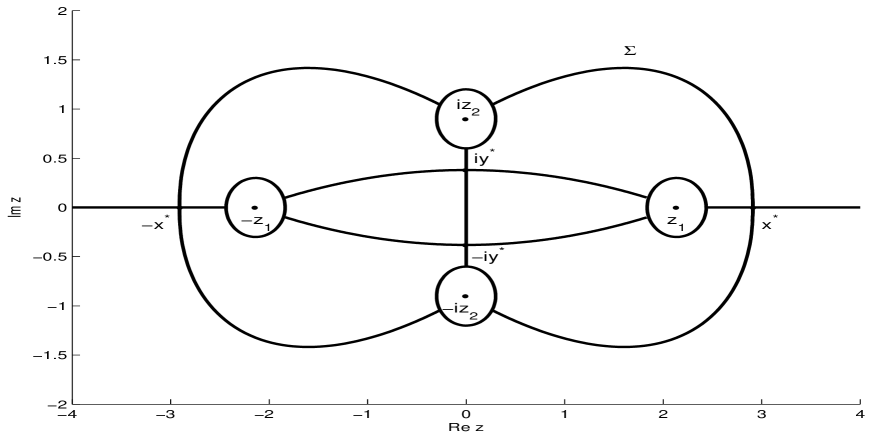
Figure 18. $R$ has jumps on this system of contours.

On the circles around the branch points there is a jump

$$R_{+}=R_{-}(I+O(1/n)),$$ (27.32)

which follows from the matching condition (27.24). On the remaining contours, the jump is

$$R_{+}=R_{-}(I+O(e^{-cn}))$$ (27.33)

for some $c>0$. Since we also have the asymptotic condition $R(z)=I+O(1/z)$ as $z\to\infty$, we may conclude as that

$$R(z)=I+O\left(\frac{1}{n(|z|+1)}\right)\qquad\mbox{ as }n\to\infty,$$ (27.34)

uniformly for $z\in\mathbb{C}$.

28. Double scaling limit at $a=1$

This section is based on the paper [BK4].

28.1. Modified Pastur equation

The analysis in the cases $a>1$ and $0<a<1$ was based on the Pastur equation (25.1), and it would be natural to use (25.1) also in the case $a=1$. Indeed, that is what we tried to do, and we found that it works for $a\equiv 1$, but in the double scaling regime $a=1+\frac{b}{2\sqrt{n}}$ with $b\neq 0$, it led to problems that we were unable to resolve in a satisfactory way. A crucial feature of our present approach is a modification of the equation (25.1) when $a$ is close to $1$, but different from $1$. At $x=0$ we wish to have a double branch point for all values of $a$ so that the structure of the Riemann surface is as in the middle figure of Figure 11 for all $a$.

For $c>0$, we consider the Riemann surface for the equation

$$z=\frac{w^{3}}{w^{2}-c^{2}}$$ (28.1)

where $w$ is a new auxiliary variable. The Riemann surface has branch points at $z^{*}=\frac{3\sqrt{3}}{2}c$, $-z^{*}$ and a double branch point at $0$. There are three inverse functions $w_{k}$, $k=1,2,3$, that behave as $z\to\infty$ as

$$w_{1}(z) =z-\frac{c^{2}}{z}+O\left(\frac{1}{z^{3}}\right)$$ (28.2)

$$w_{2}(z) =c+\frac{c^{2}}{2z}+O\left(\frac{1}{z^{2}}\right)$$

$$w_{3}(z) =-c+\frac{c^{2}}{2z}+O\left(\frac{1}{z^{2}}\right)$$

and which are defined and analytic on $\mathbb{C}\setminus[-z^{*},z^{*}]$, $\mathbb{C}\setminus[0,z^{*}]$ and $\mathbb{C}\setminus[-z^{*},0]$, respectively.

Then we define the modified $\xi$-functions

$$\xi_{k}=w_{k}+\frac{p}{w_{k}},\qquad\mbox{for }k=1,2,3,$$ (28.3)

which we also consider on their respective Riemann sheets. In what follows we take

$$c=\frac{a+\sqrt{a^{2}+8}}{4}\quad\mbox{ and }\quad p=c^{2}-1.$$ (28.4)

Note that $a=1$ corresponds to $c=1$ and $p=0$. In that case the functions coincide with the solutions of the equation (25.1) that we used in our earlier works. From (28.1), (28.3), and (28.4) we obtain the modified Pastur equation

$$\xi^{3}-z\xi^{2}+(1-a^{2})\xi+a^{2}z+\frac{(c^{2}-1)^{3}}{c^{2}z}=0,$$ (28.5)

where $c$ is given by (28.4). This equation has three solutions, with the following behavior at infinity:

$$\xi_{1}(z) =z-\frac{1}{z}+O\left(\frac{1}{z^{3}}\right),$$ (28.6)

$$\xi_{2,3}(z) =\pm a+\frac{1}{2z}+O\left(\frac{1}{z^{2}}\right),$$

and the cuts as in the middle figure of Fig.11. At zero the functions $\xi_{k}$ have the asymptotics,

$$\xi_{k}(z)=\left\{\begin{array}[]{ll}\displaystyle-\omega^{2k}z^{1/3}f_{2}(z)-\omega^{k}z^{-1/3}g_{2}(z)+\frac{z}{3}&\mbox{ for }{\operatorname{Im\,}}z>0,\\[10.0pt] \displaystyle-\omega^{k}z^{1/3}f_{2}(z)-\omega^{2k}z^{-1/3}g_{2}(z)+\frac{z}{3}&\mbox{ for }{\operatorname{Im\,}}z<0,\end{array}\right.$$ (28.7)

where the functions $f_{2}(z),g_{2}(z)$ are analytic at the origin and real for real $z$, with

$$f_{2}(0)=c^{2/3}+\frac{1}{3}c^{-4/3}(c^{2}-1),\qquad g_{2}(0)=c^{-2/3}(c^{2}-1).$$ (28.8)

We define then the functions $\lambda_{k}$ as

$$\lambda_{k}(z)=\int_{0+}^{z}\xi_{k}(s)ds$$ (28.9)

where the path of integration starts at $0$ on the upper side of the cut and is fully contained (except for the initial point) in $\mathbb{C}\setminus(-\infty,z^{*}]$, and we define the first transformation of the RHP by the same formula (26.6) as for the case $a>1$. For what follows, observe that the $\lambda$-functions have the following asymptotics at the origin:

$$\lambda_{k}(z)=\left\{\begin{array}[]{ll}\displaystyle-\frac{3}{4}\omega^{2k}z^{4/3}f_{3}(z)-\frac{1}{2}\omega^{k}z^{2/3}g_{3}(z)+\frac{z^{2}}{6}&\mbox{ for }{\operatorname{Im\,}}z>0,\\[10.0pt] \displaystyle\lambda_{k-}(0)-\frac{3}{4}\omega^{k}z^{4/3}f_{3}(z)-\frac{1}{2}\omega^{2k}z^{2/3}g_{3}(z)+\frac{z^{2}}{6}&\mbox{ for }{\operatorname{Im\,}}z<0,\end{array}\right.$$ (28.10)

where the function $f_{3}$ and $g_{3}$ are analytic at the origin and

$$f_{3}(0)=f_{2}(0)=c^{2/3}+\frac{1}{3}c^{-4/3}(c^{2}-1),\quad g_{3}(0)=3g_{2}(0)=3c^{-2/3}(c^{2}-1),$$ (28.11)

Figure 19. Lens structure for the double scaling limit.

The second transformation, the opening of lenses is given by formulas (26.9), (26.10). The lens structure is shown on Fig.19. The model solution is defined as

$$M(z)=\begin{pmatrix}M_{1}(w_{1}(z))&M_{1}(w_{2}(z))&M_{1}(w_{3}(z))\\ M_{2}(w_{1}(z))&M_{2}(w_{2}(z))&M_{2}(w_{3}(z))\\ M_{3}(w_{1}(z))&M_{3}(w_{2}(z))&M_{3}(w_{3}(z))\end{pmatrix}$$ (28.12)

where $M_{1}$, $M_{2}$, $M_{3}$ are the three scalar valued functions

$$M_{1}(w)=\frac{w^{2}-c^{2}}{w\sqrt{w^{2}-3c^{2}}},\quad M_{2}(w)=\frac{-i}{\sqrt{2}}\frac{w+c}{w\sqrt{w^{2}-3c^{2}}},\quad M_{3}(w)=\frac{-i}{\sqrt{2}}\frac{w-c}{w\sqrt{w^{2}-3c^{2}}}.$$ (28.13)

The construction of a parametrix $P$ at the edge points $\pm z^{*}$ can be done with Airy functions in the same way as for $a>1$.

28.2. Parametrix at the origin

The main issue is the construction of a parametrix at the origin, and this is where the Pearcey integrals come in. The Pearcey differential equation $p^{\prime\prime\prime}(\zeta)=\zeta p(\zeta)+bp^{\prime}(\zeta)$ admits solutions of the form

$$p_{j}(\zeta)=\int_{\Gamma_{j}}e^{-\frac{1}{4}s^{4}-\frac{b}{2}s^{2}+is\zeta}ds$$ (28.14)

for $j=0,1,2,3,4,5$, where

$$\begin{array}[]{ll}\Gamma_{0}=(-\infty,\infty),&\Gamma_{1}=(i\infty,0]\cup[0,\infty),\\ \Gamma_{2}=(i\infty,0]\cup[0,-\infty),&\Gamma_{3}=(-i\infty,0]\cup[0,-\infty),\\ \Gamma_{4}=(-i\infty,0]\cup[0,\infty),&\Gamma_{5}=(-i\infty,i\infty)\end{array}$$ (28.15)

or any other contours that are homotopic to them as for example given in Fig.20. The formulas (28.15) also determine the orientation of the contours $\Gamma_{j}$.

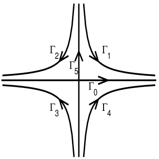
Figure 20. The contours $\Gamma_{j}$, $j=0,1,\ldots,5$, equivalent to those in (28.15), that are used in the definition of the Pearcey integrals $p_{j}$.

Define $\Phi=\Phi(\zeta;b)$ in six sectors by

$$\Phi =\begin{pmatrix}-p_{2}&p_{1}&p_{5}\\ -p_{2}^{\prime}&p_{1}^{\prime}&p_{5}^{\prime}\\ -p_{2}^{\prime\prime}&p_{1}^{\prime\prime}&p_{5}^{\prime\prime}\end{pmatrix}\qquad\textrm{ for }0<\arg\zeta<\pi/4$$ (28.16)

$$\Phi =\begin{pmatrix}p_{0}&p_{1}&p_{4}\\ p_{0}^{\prime}&p_{1}^{\prime}&p_{4}^{\prime}\\ p_{0}^{\prime\prime}&p_{1}^{\prime\prime}&p_{4}^{\prime\prime}\end{pmatrix}\qquad\textrm{ for }\pi/4<\arg\zeta<3\pi/4$$ (28.17)

$$\Phi =\begin{pmatrix}-p_{3}&-p_{5}&p_{4}\\ -p_{3}^{\prime}&-p_{5}^{\prime}&p_{4}^{\prime}\\ -p_{3}^{\prime\prime}&-p_{5}^{\prime\prime}&p_{4}^{\prime\prime}\end{pmatrix}\qquad\textrm{ for }3\pi/4<\arg\zeta<\pi$$ (28.18)

$$\Phi =\begin{pmatrix}p_{4}&-p_{5}&p_{3}\\ p_{4}^{\prime}&-p_{5}^{\prime}&p_{3}^{\prime}\\ p_{4}^{\prime\prime}&-p_{5}^{\prime\prime}&p_{3}^{\prime\prime}\end{pmatrix}\qquad\textrm{ for }-\pi<\arg\zeta<-3\pi/4$$ (28.19)

$$\Phi =\begin{pmatrix}p_{0}&p_{2}&p_{3}\\ p_{0}^{\prime}&p_{2}^{\prime}&p_{3}^{\prime}\\ p_{0}^{\prime\prime}&p_{2}^{\prime\prime}&p_{3}^{\prime\prime}\end{pmatrix}\qquad\textrm{ for }-3\pi/4<\arg\zeta<-\pi/4$$ (28.20)

$$\Phi =\begin{pmatrix}p_{1}&p_{2}&p_{5}\\ p_{1}^{\prime}&p_{2}^{\prime}&p_{5}^{\prime}\\ p_{1}^{\prime\prime}&p_{2}^{\prime\prime}&p_{5}^{\prime\prime}\end{pmatrix}\qquad\textrm{ for }-\pi/4<\arg\zeta<0$$ (28.21)

We define the local parametrix $Q$ in the form

$$Q(z)=E(z)\Phi(n^{3/4}\zeta(z);n^{1/2}b(z))e^{n\Lambda(z)}e^{-nz^{2}/6},\qquad\Lambda={\operatorname{diag}}(\lambda_{1},\lambda_{2},\lambda_{3}),$$ (28.22)

where $E$ is an analytic prefactor, and

$$\zeta(z)=\zeta(z;a)=z\left[f_{3}(z;a)\right]^{3/4}$$ (28.23)

and

$$b(z)=b(z;a)=\frac{g_{3}(z;a)}{f_{3}(z;a)^{1/2}}.$$ (28.24)

The functions $f_{3}$, $g_{3}$ appear in (28.10), in the asymptotics of the $\lambda$-functions. In (28.23) and (28.24) the branch of the fractional powers is chosen which is real and positive for real values of $z$ near $0$. The prefactor $E(z)$ is defined as

$$E(z)=-\sqrt{\frac{3}{2\pi}}ie^{-nb(z)^{2}/8}M(z)K(\zeta(z))^{-1}\begin{pmatrix}n^{1/4}&0&0\\ 0&1&0\\ 0&0&n^{-1/4}\end{pmatrix},$$ (28.25)

where

$$K(\zeta)=\left\{\begin{array}[]{ll}\begin{pmatrix}\zeta^{-1/3}&0&0\\ 0&1&0\\ 0&0&\zeta^{1/3}\end{pmatrix}\begin{pmatrix}-\omega&\omega^{2}&1\\ -1&1&1\\ -\omega^{2}&\omega&1\end{pmatrix}&\qquad\mbox{ for }{\operatorname{Im\,}}\zeta>0,\\[20.0pt] \begin{pmatrix}\zeta^{-1/3}&0&0\\ 0&1&0\\ 0&0&\zeta^{1/3}\end{pmatrix}\begin{pmatrix}\omega^{2}&\omega&1\\ 1&1&1\\ \omega&\omega^{2}&1\end{pmatrix}&\qquad\mbox{ for }{\operatorname{Im\,}}\zeta<0.\end{array}\right.$$ (28.26)

28.3. Final transformation

We fix $b\in\mathbb{R}$ and let $a=1+\frac{b}{2\sqrt{n}}$ and we define

$$R(z)=\left\{\begin{array}[]{ll}S(z)M(z)^{-1},&\textrm{ for $z\in\mathbb{C}\setminus\Sigma_{S}$ outside the disks $D(0,n^{-1/4})$ and $D(\pm\frac{3\sqrt{3}}{2},r)$},\\[10.0pt] S(z)P(z)^{-1},&\textrm{ for }z\in D(\pm\frac{3\sqrt{3}}{2},r)\setminus\Sigma_{S},\\[10.0pt] S(z)Q(z)^{-1},&\textrm{ for }z\in D(0,n^{-1/4})\setminus\Sigma_{S}.\end{array}\right.$$ (28.27)

Then $R(z)$ is analytic inside the disks and also across the real interval between the disks. Thus, $R(z)$ is analytic outside the contour $\Sigma_{R}$ shown in Fig.21.

Figure 21. The contour $\Sigma_{R}$. The matrix-valued function $R$ is analytic on $\mathbb{C}\setminus\Sigma_{R}$. The disk around $0$ has radius $n^{-1/4}$ and is shrinking as $n\to\infty$. The disks are oriented counterclockwise and the remaining parts of $\Sigma_{R}$ are oriented from left to right.

On the contour $\Sigma_{R}$ the function $R(z)$ has jumps, so that $R_{+}(z)=R_{-}(z)j_{R}(z)$, where

$$j_{R}(z) =I+O(n^{-1})\qquad\mbox{uniformly for }\left|z\mp\frac{3\sqrt{3}}{2}\right|=r,$$ (28.28)

$$j_{R}(z) =I+O(n^{-1/6})\quad\mbox{ uniformly for }|z|=n^{-1/4},$$ (28.29)

and there exists $c>0$ so that

$$j_{R}(z) =I+O\left(\frac{e^{-cn^{2/3}}}{1+|z|^{2}}\right)\quad\mbox{ uniformly for $z$ on the remaining parts of $\Sigma_{R}$.}$$ (28.30)

Also, as $z\to\infty$, we have $R(z)=I+O(1/z)$. This implies that

$$R(z)=I+O\left(\frac{n^{-1/6}}{1+|z|}\right)$$ (28.31)

uniformly for $z\in\mathbb{C}\setminus\Sigma_{R}$.

29. Concluding remarks

The Riemann-Hilbert approach is a new powerful method for random matrix models and orthogonal polynomials. In this paper we reviewed the approach and some of its applications. Let us mention some recent developments. The RH approach to orthogonal polynomials with complex exponential weights is considered in the recent work of Bertola and Mo [BM]. The RHP for discrete orthogonal polynomials and its applications is developed in the monograph [BKMM] of Baik, Kriecherbauer, McLaughlin and Miller. Applications of random matrix models to the exact solution of the six-vertex model with domain wall boundary conditions are considered in the works of Zinn-Justin [ZJ3] and Colomo and Pronko [CP]. The RH approach to the six-vertex model with domain wall boundary conditions is developed in the work of Bleher and Fokin [BF]. The RHP for a two matrix model is considered in the works of Bertola, Eynard, Harnad [BEH2] and Kuijlaars and McLaughlin [KuM2]. The universality results for the scaling limit of correlation functions for orthogonal and symplectic ensembles of random matrices are obtained in the works of Stojanovic [Sto], Deift and Gioev [DG1],[DG2], Costin, Deift and Gioev [CDG], Deift, Gioev, Kriecherbauer, and Vanlessen [DGKV].

References

- [ABK] A.I. Aptekarev, P.M. Bleher, and A.B.J. Kuijlaars, Large limit of Gaussian random matrices with external source, part II, Commun. Math. Phys. 259 (2005), 367–389.
- [Apt] A.I. Aptekarev, Multiple orthogonal polynomials, J. Comput. Math. Appl. 99, (1998), 423–447.
- [ABV] A.I. Aptekarev, A. Branquinho, and W. Van Assche, Multiple orthogonal polynomials for classical weights, Trans. Amer. Math. Soc. 355 (2003), 3887–3914.
- [AvM1] M. Adler and P. van Moerbeke, Hermitian, symmetric and symplectic random ensembles: PDEs for the distribution of the spectrum. Ann. of Math. (2) 153 (2001), no. 1, 149–189.
- [AvM2] M. Adler and P. van Moerbeke, PDEs for the joint distributions of the Dyson, Airy and sine processes. Ann. Probab. 33 (2005), no. 4, 1326–1361.
- [AvM3] M. Adler and P. van Moerbeke, PDE’s for the Gaussian ensemble with external source and the Pearcey distribution. Preprint, arxiv:math.PR/0509047.
- [BB] M. J. Bowick and E. Brézin, Universal scaling of the tail of the density of eigenvalues in random matrix models, Phys. Letts. B 268 (1991), 21–28.
- [BDE] G. Bonnet, F. David, B. Eynard, Breakdown of universality in multi-cut matrix models, J.Phys. A: Math. Gen. 33 (2000) 6739-6768.
- [BDJ] J. Baik, P. Deift, and K. Johansson, On the distribution of the length of the longest increasing subsequence of random permutations, J. Am. Math. Soc. 12 (1999) 1119-1178.
- [BDJT] R.C. Brower, N. Deo, S. Jain, and C-I Tan, Symmetry breaking in the double-well hermitian matrix models, Nucl. Phys. B405 (1993), 166–187.
- [BDT] R. Beals, P. A. Deift, and C. Tomei, Direct and inverse scattering on the line. Mathematical Surveys and Monographs 28. AMS Providence, Rhode Island (1988).
- [BE] P. Bleher and B. Eynard, Double scaling limit in random matrix models and a nonlinear hierarchy of differential equations, J. Phys. A: Math. Gen. 36 (2003) 3085-3105.
- [BEH1] M. Bertola, B. Eynard and J. Harnad, Partition functions for matrix models and isomonodromic tau functions, J. Phys. A. Math, Gen. 36 (2003) 3067-3983.
- [BEH2] M. Bertola, B. Eynard and J. Harnad, Differential systems for biorthogonal polynomials appearing in 2-matrix models and the associated Riemann-Hilbert problem, Comm. Math. Phys. 243 no.2 (2003) 193-240.
- [BEH3] M. Bertola, B. Eynard and J. Harnad, Semiclassical orthogonal polynomials, matrix models and isomonodromic tau functions, Comm. Math. Phys. 263 (2006) 401–437.
- [BF] P. Bleher and V. Fokin, Exact solution of the six-vertex model with domain wall boundary conditions. Disordered phase. Comm. Math. Phys. 268 (2006), no. 1, 223–284.
- [BH1] E. Brézin and S. Hikami, Spectral form factor in a random matrix theory, Phys. Rev. E 55 (1997), 4067–4083.
- [BH2] E. Brézin and S. Hikami, Correlations of nearby levels induced by a random potential, Nuclear Physics B 479 (1996), 697–706.
- [BH3] E. Brézin and S. Hikami, Extension of level spacing universality, Phys. Rev. E 56 (1997), 264–269.
- [BH4] E. Brézin and S. Hikami, Universal singularity at the closure of a gap in a random matrix theory, Phys. Rev. E 57 (1998) 4140–4149.
- [BH5] E. Brézin and S. Hikami, Level spacing of random matrices in an external source, Phys. Rev. E 58 (1998), 7176–7185.
- [BHZ] E. Brézin, S. Hikami, and A. Zee, Universal correlations for deterministic plus random hamiltonians, Phys. Rev. E 51 (1995), 5442.
- [BI1] P. Bleher and A. Its, Semiclassical asymptotics of orthogonal polynomials, Riemann-Hilbert problem, and universality in the matrix model. Ann. Math. 150 (1999), 185-266.
- [BI2] P. Bleher and A. Its, Double scaling limit in the random matrix model: the Riemann-Hilbert approach. Commun. Pure Appl. Math., 56 (2003), 433-516.
- [BI3] P. Bleher and A.Its, Asymptotics of the partition function of a random matrix model. Ann. Inst. Fourier 55 (2005), 1943–2000.
- [BIPZ] E. Brézin, C. Itzykson, G. Parisi, and J.-B. Zuber, Planar diagrams Commun. Math. Phys. 59 (1978), 35–51.
- [BIZ] D. Bessis, C. Itzykson, and J.-B. Zuber, Quantum field theory techniques in graphical enumeration, Adv. Applied Math. 1 (1980), 109–157.
- [BK1] P.M. Bleher and A.B.J. Kuijlaars, Random matrices with external source and multiple orthogonal polynomials, Int. Math. Research Notices 2004, no 3 (2004), 109–129.
- [BK2] P.M. Bleher and A.B.J. Kuijlaars, Large limit of Gaussian random matrices with external source, part I, Commun. Math. Phys. 252 (2004), 43–76.
- [BK3] P.M. Bleher and A.B.J. Kuijlaars, Integral representations for multiple Hermite and multiple Laguerre polynomials, Ann. Inst. Fourier 55 (2005), 2001–2004.
- [BK4] P.M. Bleher and A.B.J. Kuijlaars, Large limit of Gaussian random matrices with external source, part III: Double scaling limit, Commun. Math. Phys. 270 (2006), 481 517.
- [BKMM] J. Baik, T. Kriecherbauer, K.T.-R. McLaughlin, and P.D. Miller, Discrete orthogonal polynomials: Asymptotics and applications (AM-164), Princeton University Press, 2006.
- [BM] M. Bertola and M. Y. Mo, Commuting difference operators, spinor bundles and the asymptotics of pseudo-orthogonal polynomials with respect to varying complex weights, arXiv:math-ph/0605043.
- [BPS] A. Boutet de Monvel, L. A. Pastur, and M. Shcherbina, On the statistical mechanics approach in the random matrix theory. Integrated density of states, J. Statist. Phys. 79 (1995), 585–611.
- [BrK] E. Brézin and V. A. Kazakov, Exactly solvable field theories of closed strings, Phys. Lett. B 236 (1990), 144–150.
- [BZ] E. Brézin and A. Zee, Universality of the correlations between eigenvalues of large random matrices, Nuclear Physics B 402 (1993), 613–627.
- [CDG] O. Costin, P. Deift and D. Gioev, On the proof of universality for orthogonal and symplectic ensembles in random matrix theory. Preprint, arXiv:math-ph/0610063.
- [CDM] C. Crnkovic, M. Douglas, and G. Moore. Loop equations and the topological phase of multi-cut matrix models, Int. J. Mod. Phys. A7 (1992) 7693-7711.
- [ChG] Y. Chen and T. Grava. Eigenvalue correlations on hyperelliptic Riemann suefaces, J. Phys. A: Math. Gen. 35 (2002) L45-L49.
- [CI1] Y. Chen and M. Ismail. Ladder operators and differential equations for orthogonal polynomials, J. Phys. A: Math. Gen. 30 (1997) 7817-7829.
- [CI2] Y. Chen and M. Ismail. Thermodynamic relations of the Hermitian matrix ensembles, J. Phys. A: Math. Gen. 30 (1997) 6633-6654.
- [CG] K. Clancey and I. Gohberg, Factorization of matrix functions and singular integral operators. Operator Theory. 3, Birkhäuser Verlag Basel (1981).
- [CK] T. Claeys and A.B.J. Kuijlaars, Universality of the double scaling limit in random matrix models, Commun. Pure Appl. Math. 59 (2006) 1573-1603.
- [CKV] T. Claeys, A.B.J. Kuijlaars, and M. Vanlessen, Multi-critical unitary random matrix ensembles and the general Painlevé II equation, arxiv:math-ph/0508062 (to appear in Ann. Math.).
- [CP] F. Colomo and A. G. Pronko, Square ice, alternating sign matrices, and classical orthogonal polynomials, J. Stat. Mech. Theory Exp. 2005, no. 1, 005, 33 pp. (electronic).
- [DDJT] K. Demeterfi, N. Deo, S. Jain, and C.-I Tan, Multiband structure and critical behavior of matrix models, Phys. Rev. D, 42 (1990) 4105-4122.
- [Dei] P. Deift, Orthogonal Polynomials and Random Matrices: a Riemann-Hilbert Approach. Courant Lecture Notes in Mathematics, 3. Amer. Math. Soc., Providence RI, 1999.
- [DG1] P. Deift and D. Gioev, Universality in random matrix theory for orthogonal and symplectic ensembles. Preprint, arXiv: math-ph/0411057.
- [DG2] P. Deift and D. Gioev, Universality at the edge of the spectrum for unitary, orthogonal and symplectic ensembles of random matrices. Preprint, arXiv: math-ph/0507023, to appear in Comm. Pure Appl. Math.
- [DGKV] P. Deift, D. Gioev, T. Kriecherbauer, and M. Vanlessen, Universality for orthogonal and symplectic Laguerre-type ensembles. Preprint, arXiv:math-ph/0612007.
- [DGZ] Ph. Di Francesco, P. Ginsparg, and J. Zinn-Justin, D gravity and random matrices, Phys. Rep. 254 (1995) no. 1-2, 133 pp.
- [DiF] P. Di Francesco, Matrix model combinatorics: applications to folding and coloring. In: “Random Matrices and Their Applications”, MSRI Publications 40. Eds. P. Bleher and A. Its, Cambridge Univ. Press (2001), 111-170.
- [DK] E. Daems and A.B.J. Kuijlaars, A Christoffel-Darboux formula for multiple orthogonal polynomials, J. Approx. Theory 130 (2004), 190–202.
- [DKM] P. A. Deift, T. Kriecherbauer, K. T-R. McLaughlin, New results on equilibrium measure for logarithmic potentials in the presence of an external field. J. Approx. Theory 95 (1998), 388-475.
- [DKMVZ] P. Deift, T. Kriecherbauer, K.T-R McLaughlin, S. Venakides, and X. Zhou, Strong asymptotics of orthogonal polynomials with respect to exponential weights, Comm. Pure Appl. Math. 52 (1999), 1491–1552.
- [DKMVZ2] P. A. Deift, T. Kriecherbauer, K. T-R. McLaughlin, S. Venakides, and Z. Zhou, Uniform asymptotics for polynomials orthogonal with respect to varying exponential weights and applications to universality questions in random matrix theory. Commun. Pure Appl. Math. 52 (1999), 1335-1425.
- [DS] M. Douglas, S. Shenker, Strings in less than one dimension. Nuclear Phys. B 335 (1990), no. 3, 635–654.
- [DSS] M. Douglas, N. Seiberg, and S. Shenker, Flow and instability in quantum gravity, Phys. Lett. B 244 (1990), 381–386.
- [Dub] B. A. Dubrovin, Theta functions and non-linear equations, Russian Math. Surveys 36:2 (1981), 11–92.
- [DuK] M. Duits and A. Kuijlaars, Painleve I asymptotics for orthogonal polynomials with respect to a varying quartic weight, Nonlinearity 19 (2006), 2211-2245.
- [DZ] P. Deift and X. Zhou, A steepest descent method for oscillatory Riemann-Hilbert problems. Asymptotics for the MKdV equation, Ann. Math. 137 (1993), 295–368.
- [Dys] F. J. Dyson, Correlation between the eigenvalues of a random matrix, Commun. Math. Phys. 19, 235–250 (1970).
- [EM] N.M. Ercolani and K.D.T-R McLaughlin, Asymptotics of the partition function for random matrices via Riemann-Hilbert techniques and applications to graphical enumeration. Int. Math. Res. Not. 14 (2003), 755–820.
- [EMP] N.M. Ercolani, K.D.T-R McLaughlin, and V.U. Pierce, Random matrices, graphical enumeration and the continuum limit of Toda lattices. Preprint, arXiv:math-ph/0606010.
- [Eyn1] B. Eynard, Eigenvalue distribution of large random matrices, from one matrix to several coupled matrices, Nucl. Phys. B 506 (1997), 633-664.
- [Eyn2] B. Eynard, A concise expression for the ODE’s of orthogonal polynomials. Preprint, arXiv:math-ph/0109018.
- [FIK] A. S. Fokas, A. R. Its, and A. V. Kitaev, The isomonodromy approach to matrix models in 2D quantum gravity, Commun. Math. Phys. 147, 395–430 (1992).
- [FK] H.M. Farkas and I. Kra, Riemann Surfaces (Graduate Texts in Mathematics), 2nd ed., Springer, 1991.
- [FIK0] A. R. Its, A. V. Kitaev, A. S. Fokas, Matrix models of two-dimensional quantum gravity and isomonodromy solutions of “discrete Painlevé equations”. Zap. Nauch. Sem. LOMI 187 3 - 30 (1991) (Russian), translation in J. Math. Sci. 73, 4 415 - 429 (1995)
- [For] P. J. Forrester, The spectrum edge of random matrix ensembles, Nucl. Phys. B402, 709–728 (1993).
- [GM] D. Gross and A. Migdal, Nonperturbative two-dimensional quantum gravity, Phys. Rev. Lett. 64 (1990) 127-130; A nonperturbative treatment of two-dimensional quantum gravity, Nucl. Phys. B 340 (1990) 333–365.
- [GW] D. Gross and E. Witten, Possible third-order phase transition in the large- lattice gauge theory, Phys. Rev. D 21 (1980) 446-453.
- [HMPN] T. Hollowood, L. Miramontes, A. Pasquinucci, and C. Nappi, Hermitian versus anti-hermitian one-matrix models and their hierarchies, Nucl. Phys. B 373 (1992) 247-280.
- [IKO] A.R. Its, A.B.J. Kuijlaars, and J. Östensson, Critical edge behavior in unitary random matrix ensembles and the thirty fourth Painleve transcendent, arXiv:0704.1972.
- [IN] A. Its and V. Novokshenov, The isomonodromic deformation method in the theory of Painlevé equations, Lecture Notes in Math. 1191 (1986), Springer-Verlag, New York.
- [IZ] C. Itzykson and J.-B. Zuber, The planar approximation. II, J. Math. Phys., 21, 411–421 (1980).
- [Joh] K. Johansson, On fluctuations of eigenvalues of random hermitian matrices, Duke Math. J. 91 (1988), 151–204.
- [Kit] A. Kitaev, Turning points of linear systems and double asymptotics of Painlevé transcendents, Diff. Geom. Lie Groups Mech. 12, LOMI 187 (1991) 53-74.
- [KrM] T. Kriecherbauer, K. T-R. McLaughlin, Strong asymptotics of polynomials orthogonal with respect to Freud weights. Internat. Math. Res. Notices 6 (1999), 299-333.
- [Kui] A.B.J. Kuijlaars, Riemann-Hilbert analysis for orthogonal polynomials, in: Orthogonal Polynomials and Special Functions (E. Koelink and W. Van Assche eds), Lecture Notes in Mathematics Vol. 1817, Springer-Verlag, 2003, pp. 167–210.
- [KuM1] A.B.J. Kuijlaars and K.T-R McLaughlin, Generic behavior of the density of states in random matrix theory and equilibrium problems in the presence of real analytic external fields. Comm. Pure Appl. Math. 53 (2000), 736–785.
- [KuM2] A.B.J. Kuijlaars and K.T-R McLaughlin, A Riemann-Hilbert problem for biorthogonal polynomials, J. Comput. Appl. Math. 178 (2005) 313 - 320.
- [LiS] G. Litvinchuk and T. Spitkovskii, Factorization of measurable matrix functions. Birkhäuser Verlag, Basel, 51 (1987).
- [Meh] M. L. Mehta, Random Matrices, 2nd ed., Academic Press, Boston, 1991.
- [Moo1] G. Moore, Matrix models of 2D gravity and isomonodromic deformations, Progr. Theor. Phys. Suppl., 102 (1990), 255.
- [Moo2] G. Moore, Geometry of the string equations, Commun. Math. Phys. 133 (1990) 261-304.
- [OR] A. Okounkov and N. Reshetikhin, Random skew plane partitions and the Pearcey process, arxiv:math.CO/0503508.
- [Pas] L.A. Pastur, The spectrum of random matrices (Russian), Teoret. Mat. Fiz. 10 (1972), 102–112.
- [PaS] L. Pastur and M. Shcherbina, Universality of the local eigenvalue statistics for a class of unitary invariant random matrix ensembles, Journ. Statist. Phys. 86, 109–147 (1997).
- [Pea] T. Pearcey, The structure of an electromagnetic field in the neighborhood of a cusp of a caustic, Philos. Mag. 37 (1946), 311–317.
- [PeS] V. Periwal and D. Shevitz, Exactly solvable unitary matrix models: multicritical potentials and correlations, Nucl. Phys. B333 (1990), 731.
- [ST] E.B. Saff and V. Totik, Logarithmic Potentials with External Field, Springer-Verlag, 1997.
- [Sto] A. Stojanovic, Universality in orthogonal and symplectic invariant matrix models with quartic potential. Math. Phys. Anal. Geom. 3 (2000), 339 373. Errata: ibid., 7 (2004), 347 349.
- [Sze] G. Szego, Orthogonal Polynomials. Fourth edition. Colloquium Publications, vol. 23, AMS, Providence, RI, 1975.
- [TW1] C. A. Tracy and H. Widom, Introduction to random matrices, In: Geometric and quantum aspects of integrable systems (Scheveningen, 1992), 103–130, Lecture Notes in Phys. 424, Springer, Berlin, 1993.
- [TW2] C. A. Tracy and H. Widom, Level-spacing distribution and the Airy kernel, Commun. Math. Phys. 159 (1994) 151–174.
- [TW3] C. Tracy and H. Widom, The Pearcey process, Commun. Math. Phys. 263 (2006) 381-400.
- [TW4] C. Tracy and H. Widom, Nonintersecting Brownian excursions, arXiv:math/0607321arXiv:math/0607321 (to appear in Ann. Appl. Probab.).
- [VAGK] W. Van Assche, J.S. Geronimo, and A.B.J. Kuijlaars, Riemann-Hilbert problems for multiple orthogonal polynomials, pp. 23–59 in: ”NATO ASI Special Functions 2000. Current Perspective and Future Directions”, (J. Bustoz, M.E.H. Ismail, S.K. Suslov eds.), Nato Science Series II Vol.30, Kluwer Academic Publishers, Dordrecht, 2001.
- [Wit] E. Witten, Two-dimensional gravity and intersection theory on moduli spaces, Surveys in differential geometry (Cambridge, MA, 1990), 243–310, Lehigh Univ., Bethlehem, PA, 1991.
- [Zh] X. Zhou, Riemann-Hilbert problem and inverse scattering, SIAM J. Math. Anal. 20, 966–986 (1989).
- [ZJ1] P. Zinn-Justin, Random Hermitian matrices in an external field, Nuclear Physics B 497 (1997), 725–732.
- [ZJ2] P. Zinn-Justin, Universality of correlation functions of Hermitian random matrices in an external field, Comm. Math. Phys. 194 (1998), 631–650.
- [ZJ3] P. Zinn-Justin, Six-vertex model with domain wall boundary conditions and one-matrix model. Phys. Rev. E 62 (2000), 3411-3418.