Global disease spread: statistics and estimation of arrival times

Abstract

We study metapopulation models for the spread of epidemics in which different subpopulations (cities) are connected by fluxes of individuals (travelers). This framework allows to describe the spread of a disease on a large scale and we focus here on the computation of the arrival time of a disease as a function of the properties of the seed of the epidemics and of the characteristics of the network connecting the various subpopulations. Using analytical and numerical arguments, we introduce an easily computable quantity which approximates this average arrival time. We show on the example of a disease spread on the world-wide airport network that this quantity predicts with a good accuracy the order of arrival of the disease in the various subpopulations in each realization of epidemic scenario, and not only for an average over realizations. Finally, this quantity might be useful in the identification of the dominant paths of the disease spread.

,

1 Introduction

In our modern world, the existence of various transportation means has strongly affected the way in which infectious diseases spread among humans. In fact, it has become unavoidable to take into account in the study of the geographical spread of epidemics the various long-range heterogeneous connections typical of modern transportation networks, This naturally gives rise to a very complicated evolution of epidemics characterized by heterogeneous outbreaks patterns (Cohen,, 2000; Cliff & Haggett,, 2004; Colizza et al., 2006a, ; Colizza et al., 2006b, ), as recently documented at the world-wide level in the SARS case (http://www.who.int/csr/sars/en).

Such complex phenomenon can be tackled at different granularity levels, including very detailed agent-based simulations, complicated social and spatial structures, complex contact networks, etc. (Anderson & May,, 1992; Hethcote & Yorke,, 1984; Kretzschmar & Morris,, 1996; Keeling,, 1999; Pastor-Satorras & Vespignani, 2001a, ; Pastor-Satorras & Vespignani, 2001b, ; May & Lloyd, 2001; Ferguson et al.,, 2003; Meyers et al.,, 2005; Chowell et al.,, 2003; Eubank et al.,, 2004). In particular, a very important class of models in modern epidemiology describes the propagation between different interconnected subpopulations with the help of the so-called metapopulation models. In these models, the disease spreads inside each subpopulation (often assumed homogeneously mixed) and is transmitted between different subpopulations by a “coupling” depending on the model. In the case of human infectious diseases, this coupling is caused by the movements of individuals and depends on the transportation means relevant at the spatial scale chosen for the description of the spread.

In the context of large scale spread, air-transportation represents a major channel of epidemic propagation, as pointed out in the modeling approach to global epidemic diffusion of Rvachev and Longini (Rvachev & Longini,, 1985; Baroyan et al.,, 1969) and by similar studies on the behavior of specific outbreaks such as pandemic influenza, HIV or SARS (Longini,, 1988; Grais et al.,, 2003; Brownstein et al.,, 2006; Flahault & Valleron,, 1992; Hufnagel et al.,, 2004; Colizza et al., 2006a, ; Colizza et al., 2006b, ; Colizza et al., 2007a, ). In this case, the relevant metapopulation model considers as subpopulations the inhabitants of the various world cities and the air travel of infectious individuals results in the spread of the disease from one city to another.

Taking into account the global airline transportation infrastructure in metapopulation models has recently become possible thanks to the availability and analysis of large scale databases (Barrat et al.,, 2004; Guimerà et al.,, 2005), and to the always increasing computer capacities. The word wide airport network (WAN) is described by a complex weighted graph, in which the airports are the vertices and the weighted links represent the presence of direct flight connections among them (the weights corresponding to the number of available seats on each connection). This network, which consists of more than $3000$ nodes and $18000$ links, displays small-world properties as well as strongly heterogeneous topology and traffic properties. For many different dynamical phenomena occurring on complex networks (Albert & Barabási,, 2002; Dorogovtsev & Mendes,, 2003; Pastor-Satorras & Vespignani,, 2004; Boccaletti et al.,, 2006), the presence of such emerging properties has been shown to imply the breakdown of the standard results. This is particularly true for epidemiology  (Pastor-Satorras & Vespignani, 2001a, ; Pastor-Satorras & Vespignani, 2001b, ; May & Lloyd, 2001) where classical results about epidemic thresholds do not apply if the heterogeneity of the network is too large. This therefore calls for a systematic investigation of the epidemic spread in the framework of metapopulation models defined on complex networks such as the world airport network. Such investigations can be carried out in various parallel and complementary directions. On the one hand, the availability of large scale datasets has recently allowed for the development of tools for intensive computational epidemiology (Colizza et al., 2006a, ; Colizza et al., 2006b, ; Colizza et al., 2007a, ), which can be used for example for scenario evaluations (Colizza et al., 2007a, ) and risk assessment. On the other hand, these computational tools can also be used for the study of fundamental properties of these metapopulation models, and to understand the main mechanisms of the disease spread and the role of the various complex properties of the transport network. In particular, Colizza et al., 2006a ; Colizza et al., 2006b have investigated how the properties of the global air travel network affect the heterogeneity and the predictability of spreading patterns. Very recently moreover, the effect on the epidemic threshold of both the network properties and the endogenous reaction was studied using analytical and numerical tools typical of statistical physics (Colizza et al., 2007b, ; Colizza & Vespignani,, 2007).

In this paper, we tackle the problem of determining the arrival time of an epidemics spread in a metapopulation model consisting in subpopulations (cities) coupled by a transportation network. We stress that this study is different from the ones of Crépey et al., (2006) and Barthélemy et al., (2005), in which each node of the network is an individual (and not a full subpopulation), and where links represent the possibility of the contamination between individuals. The main result of the present paper is to exhibit an easily computable quantity depending only on the networks characteristics and which approximates the average arrival time. This quantity is only an approximation of the exact arrival time but we show on the example of the world-wide disease spread that it allows to rank the cities according to the arrival of the disease.

The paper is organized as follows. We present in section 2 the Rvachev-Longini metapopulation model for the epidemics spreading, and in section 3, we study the arrival time of a disease for simple topologies such as a one-dimensional line of cities. We then extend these results to the case of complex networks and we propose a quantity which is a good approximation to the average arrival time in the various nodes or subpopulations connected through an arbitrary network of connections. We finally show in section 4, using numerical simulations of epidemic spreading on the worldwide airport network, that our approximation is not only valid for the average arrival time, but is also able to give the order of arrival of the disease in the various cities with a good precision for each spreading realization. A brief account of some of the results presented here can be found in (Gautreau et al.,, 2007).

2 The Rvachev-Longini metapopulation model

The Rvachev-Longini model (Rvachev & Longini,, 1985) was initially introduced to describe the spread of the 1968-69 Hong-Kong flu at the worldwide level. This metapopulation model uses two different levels of description: the various subpopulations are given by the inhabitants of the $58$ large cities corresponding to the $58$ largest airports, and homogeneous mixing is assumed at the individual city level. In this model, the propagation of the disease from one subpopulation to another is due to individuals traveling on the air-transportation network between these airports (Rvachev & Longini,, 1985).

The evolution of the number $I_{i}$ of infectious individuals in each city $i$ can thus be written as the sum of two terms

$$\partial_{t}I_{i}=K(\{X_{i}\})+\Omega(\{I_{j}\})\ ,$$ (1)

where the first term $K$ of the rhs describes the (epidemic) reaction process inside each subpopulation (city), due to the interaction of individuals in the various possible states $X$ ($X=S,L,I,R...$ depending on the population compartimentalization into Susceptible, Latent, Infected, Recovered… individuals). The second term of the rhs represents the incoming and outgoing fluxes of infectious individuals to and from other cities $j$. This model therefore considers a simplified mechanistic approach with a markovian assumption in which individuals are not labeled according to their original subpopulation, and where at each time step the same traveling probability applies to all individuals in the subpopulation, without any memory of their previous locations (Rvachev & Longini,, 1985; Hufnagel et al.,, 2004; Colizza et al., 2006a, ; Colizza et al., 2006b, ). The travel term $\Omega$ depends therefore on the air-transportation network: if the weight $w_{ij}$ represents the number of passengers traveling from $i$ to $j$ per unit of time ($w_{ij}=0$ if there is no direct connection between $i$ and $j$), and $N_{i}$ the population of the city $i$, it is reasonable to assume that the probability per unit time that an individual in city $i$ travels to city $j$ is given by $w_{ij}/N_{i}$. In the case of a simple SI model, the time evolution of the number $I_{i}$ of infectious infividuals in city $i$ is therefore given by:

$$\partial_{t}I_{i}=\lambda I_{i}\left(t\right)\frac{N_{i}-I_{i}\left(t\right)}{N_{i}}+\sum_{j}\frac{w_{ji}}{N_{j}}I_{j}-\sum_{j}\frac{w_{ij}}{N_{i}}I_{i}\ ,$$ (2)

where $\lambda$ is the transmission rate. Similar equations can be written for the other compartments in the various possible models (SIS, SIR…), by modifying the first term $K$ of the rhs in Eq. (2) accordingly.

This original formulation has an important drawback. Indeed, it is deterministic, since it considers only expectation values, while both epidemic spreading and travel of individuals are inherently stochastic processes. The number of infectious individuals is then treated as a continuous variable and, even if the initial condition (at $t=0$) of the spreading consists in one single infectious individual in a given city $i_{0}$, all cities have a non-zero density of infectious at any time $t>0$. In order to tackle the problem of the arrival time of the spread in the various subpopulations, this pathology has to be accounted for. A first possibility, already presented by Rvachev & Longini, (1985), to avoid this unrealistic situation consists in considering that each travel term $w_{ij}I_{i}/N_{i}$ is present only when $w_{ij}I_{i}/N_{i}>1$, i.e. in putting a threshold term $\theta(w_{ij}I_{i}/N_{i}-1)$, corresponding to the fact that the expected number of travelers has to be larger than unity. In this approach however the “quantity” of individuals traveling is still a continuous variable. Another possibility, which consists in treating all quantities as integers and going back to the microscopic stochastic processes, can be necessary for detailed modeling purposes (Colizza et al., 2007a, ). This solution is however computationally quite demanding, so that we will consider in all numerical simulations performed in this paper an intermediate framework: the travel term is treated as in the stochastic generalization described by Colizza et al., 2006a ; Colizza et al., 2006b (see also Hufnagel et al., (2004)), where the number of individuals traveling on each connection is an integer variable randomly extracted at each time step. More precisely, each of the $[I_{i}]$ (the integer part of $I_{i}$) infectious individuals has a probability $p_{ij}=w_{ij}\Delta t/N_{i}$ to go from $i$ to $j$ in the time interval $\Delta t$. The numbers $\xi_{ij}$ of infectious individuals traveling on the various connections existing from $i$ to other cities $j$ are given by a set of stochastic variables which follow then a multinomial distribution (Colizza et al., 2006b, )

$$P\left(\{\xi_{ij}\}\mid\{I_{i}\}\right)=\frac{[I_{i}]!}{\left([I_{i}]-\sum_{j}\xi_{ij}\right)!\prod_{j}\xi_{ij}!}\times\prod_{j}p_{ij}^{\xi_{ij}}\left(1-\sum_{j}p_{ij}\right)^{[I_{i}]-\sum_{j}\xi_{ij}}$$ (3)

where the mean and variance of the stochastic variables are $\langle\xi_{ij}\left([I_{i}]\right)\rangle=w_{ij}\Delta t[I_{i}]/N_{i}$ and $Var\left(\xi_{ij}\right)=\frac{w_{ij}}{N_{i}}\Delta t\left(1-\frac{w_{ij}}{N_{i}}\Delta t\right)[I_{i}]$. On the other hand, the endogenous growth (inside each city) will be treated for simplicity as a deterministic evolution of densities of infectious and susceptible individuals. We have moreover checked numerically that the inclusion of stochastic effects described by noise terms in the evolution equations (Colizza et al., 2006a, ; Colizza et al., 2006b, ) do not change our results. Finally, we will present the results essentially for the simple SI model, since arrival times will basically depend on the first stage of the disease development. We have however carried out numerical simulations as well in the SIS and SIR case, with consistent results (see section 4).

It is interesting to note that in realistic cases such as a disease propagation on the WAN, most weights are symmetric ($w_{ij}=w_{ji}$) (Barrat et al.,, 2004) but the probabilities of travel from one city to another are not ($p_{ij}\neq p_{ji}$). The travel therefore effectively occurs as a random diffusion on a directed weighted complex network. Moreover, an important difference with the case of random walks on complex networks (Noh & Rieger,, 2003) comes from the endogenous evolution inside each subpopulation. Indeed, as soon as an infectious individual reaches a city, a contamination process starts and the number of random infectious walkers is not constant. Such an intricate behavior has also important consequences on the existence of epidemic thresholds, as studied recently by Colizza et al., 2007b .

As a last general remark, we note that the simple topological distance between nodes should naturally play a role in the context of arrival times, but does not contain all the information needed to characterize such a process, nor does a priori the optimal weighted distance, which takes into account the weights (Wu et al.,, 2006) but not the populations nor the endogenous epidemic evolution. Moreover, since most transportation networks are small-world networks (even when taking into account weights), many cities lie at the same topological distance from a given seed, but will be reached at very different times.

3 Arrival times statistics

In this section, we study the arrival time of the first infectious individual in the various cities, starting with very simple topologies for the transportation network.

3.1 Two cities : arrival time distribution

We start with the case of two connected cities ($0$ and $1$). We denote the link weight by $w_{01}=w$, the population of the first city by $N_{0}=N$, the number of infectious individuals in city $0$ by $I_{0}=I$. The probability to jump from $0$ to $1$ during the time interval $\Delta t$ is $p=\frac{w}{N}\Delta t$. The initial condition is given by $I_{0}(t=0)=I^{0}$, $I_{1}(t=0)=0$, i.e., infectious individuals are present only in city $0$. We consider that the travel events occur as instantaneous jumps (of probability $p$ for each individual) at discretized times. The probability that the first infectious individual arrives at time $t_{1}=t=n\Delta t$ in city $1$ is then given by

$$P\left(t_{1}=n\Delta t\right)=\left(1-\left(1-p\right)^{{[I_{0}(n\Delta t)]}}\right)\times\prod_{i=1}^{n-1}\left(1-p\right)^{{[I_{0}(i\Delta t)]}}\ ,$$ (4)

which expresses the fact that at least one successful “jump” from $0$ to $1$ of an infectious individual occurs at time $n\Delta t$, and none at previous times. In Eq. (4), the quantity $[I_{0}]$ denotes the integer part of $I_{0}$. In order to obtain the probability density of the arrival time in city $1$, we first note that in real-world systems the number of travelers is usually small with respect to the total population of a city: $p=w\Delta t/N\ll 1$ (with any reasonable $\Delta t$). In this limit, Eq. (4) becomes

$$P\left(t_{1}=t\right)=p[I_{0}(t)]e^{-p\sum_{0<i<n}{[I_{0}\left(i\Delta t\right)]}}\ .$$ (5)

We will also assume that the travel probability is sufficiently small so that the number of infectious individuals $I_{0}(t)$ in the city $0$ grows substantially before the city $1$ is contaminated. Writing $1\ll I_{0}(t)\ll N$ (the second inequality is due to the fact that in realistic cases only small fractions of the population are contaminated), we thus consider the following approximation: $[I](t)\approx I_{0}(t)\approx I^{0}e^{\lambda t}$ (as long as $t<t_{1}$). Using as well the standard approximation $\Delta t\sum_{0<i<n}[I_{0}\left(i\Delta t\right)]=\int_{0}^{t}I_{0}\left(\tau\right)d\tau$, we obtain for $I^{0}=1$

$$P(t)dt=\frac{w}{N}e^{\lambda t-\frac{w}{N\lambda}e^{\lambda t}}\Theta(t)dt\ ,$$ (6)

where $\Theta(t)$ is the Heavyside function which ensures the positivity of the arrival time. The distribution (6) is a Gumbel distribution with average $\langle t_{1}\rangle=\frac{1}{\lambda}\left(\ln\left(\frac{N\lambda}{w}\right)-\gamma\right)$, where $\gamma$ is the Euler constant. The contribution of the negative $t$ in the distribution has to be negligible before $1$, which reads $\int_{-\infty}^{0}P\left(t\right)dt=\frac{w}{N\lambda}\ll 1$. This range of validity corresponds also to the hypothesis of $\lambda\langle t_{1}\rangle\gg 1$ (the time to increase $I_{0}$ by one individual is small with respect to the time scale of the epidemic arrival in city $1$).

Figure 1 displays the results of numerical simulations of the propagation between two cities, using discrete stochastic travel events as described in section 2. The whole distribution of arrival times in the second city shows a very good agreement with the form (6), obtained through the continuous approximations detailed above. When $w/(N\lambda)$ is not small enough, stronger deviations are obtained; this is expected since the hypothesis $1\ll I_{0}(t)$ for $t<t_{1}$ is less valid. Nonetheless, the overall shape of the distribution is still in good agreement (Inset of Fig. 1).

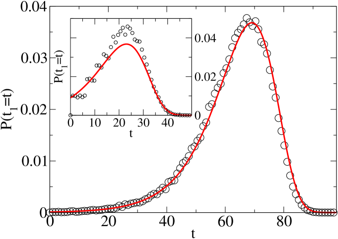
Figure 1: Two cities model, distribution of arrival times $t^{\left(1\right)}$ in numerical simulations with $\frac{w}{N\lambda}=10^{-2}$. Inset : distribution of $t^{\left(1\right)}$ with $\frac{w}{N\lambda}=10^{-1}$. The continuous line is the analytical approximation given by Eq. (6). Here and in the following, unless specified, $N=10^{6}$ and $\lambda=0.1$.

3.2 One-dimensional line

We now consider a one-dimensional line of subpopulations $i\geq 0$, with an initial condition given by one infectious individual in city $0$. We denote by $w_{i}$ the travel flux between city $i$ and city $i+1$, $t_{i}$ the arrival time of the first infectious in city $i$, and $\Delta_{i}=t_{i}-t_{i-1}$ ($t_{0}=0$). The quantity $t_{n}$ is thus the sum of the random variables $\Delta_{i}$ for $i=1,...,n$, and the average is given by $\langle t_{n}\rangle=\sum_{i=1,...,n}\langle\Delta_{i}\rangle$. These random variables $\Delta_{i}$ are a priori correlated and not identically distributed which implies that the central limit theorem can not be used in general.

Homogeneous line

In the case of a homogeneous line with uniform populations and weights ($N_{i}=N$, $w_{i}=w$), one expects that the distributions of $\Delta_{n}$ becomes independent of $n$ at large $n$, with a well-defined average $\lim_{n\to\infty}\langle\Delta_{n}\rangle=\langle\Delta\rangle$, so that $t_{n}\approx n\langle\Delta\rangle$. The issue then is the computation of $\langle\Delta\rangle$. Two time scales only are present: $N/w$ which represents the average time for an individual to travel from one city to the next, and $1/\lambda$ which represents the typical transmission time of the disease. Dimensional analysis thus implies that the adimensional quantity $\lambda\langle\Delta\rangle$ has the form

$$\lambda\langle\Delta\rangle=F\left(\frac{w}{N\lambda}\right)\ .$$ (7)

In order to estimate the unknown function $F$, a first possibility is to consider that at large $n$ the spread consists in an evolving epidemic front obeying the continuous equation $\partial_{t}I(x,t)=\lambda SI+w\partial^{2}_{x}I(x,t)$. Looking for a traveling wave solution (Murray,, 2004) leads to a front speed $v=2\sqrt{\frac{\lambda w}{N}}$, and thus to

$$\langle\Delta\rangle_{front}\approx\frac{1}{2\lambda}\sqrt{\frac{N\lambda}{w}}\ .$$ (8)

Another possibility consists in using the results of the previous subsection, and assume that the average of $\Delta_{n}$ remains close to the arrival time in the first city $\langle\Delta_{n}\rangle\approx\langle\Delta_{1}\rangle=\langle t_{1}\rangle$ which yields

$$\langle\Delta\rangle_{Gumbel}=\frac{1}{\lambda}\left[\ln\left(\frac{N\lambda}{w}\right)-\gamma\right]\ .$$ (9)

This approximation neglects the fact that $I_{n-1}(t)$ increases between $t_{n-1}$ and $t_{n}$ due both to the endogeneous growth in city $n-1$ and to the arrival of infectious individuals from city $n-2$, while for the computation of $\langle t_{1}\rangle$, only the endogeneous growth of $I_{0}$ has to be considered. It can therefore be expected that $\langle\Delta\rangle_{Gumbel}$ will overestimate the real $\langle\Delta\rangle$.

Finally, we can also consider a deterministic formulation, in which travel between $i$ and $i+1$ occurs only if there are enough infectious individuals in $i$, i.e. $I_{i}(t)$ has reached a certain threshold $\theta$, and is then treated as continuous. In this framework, each city is considered infected only if the number of infectious individuals is above $\theta$, and $t_{n}$ is defined as the first time that $I_{n}$ reaches the threshold: $I_{n}(t_{n})=\theta$. Between $t_{n-1}$ and $t_{n}$, no travel can therefore occur out of $n$, and we can write $\partial_{t}I_{n}=\lambda I_{n}+\frac{w}{N}I_{n-1}$. During $[t_{n-1},t_{n}]$, under the realistic hypothesis that $I_{n}\ll N_{n}$, and that $I_{n-1}$ is in a first approximation given by $I_{n-1}=e^{\lambda\left(t-t_{n-1}\right)}$, we obtain the equation $1=\frac{w}{N}\Delta_{n}e^{\lambda\Delta_{n}}$. The difference between the arrival times in two successive cities is therefore given by

$$\langle\Delta\rangle_{det}=\frac{1}{\lambda}W\left(\frac{N\lambda}{w}\right)$$ (10)

where $W$ is known as the Lambert W function.

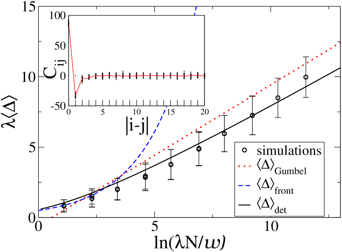
Figure 2: Slope $\langle\Delta\rangle$ of $\langle t_{n}\rangle$ vs $n$ on a line of length $500$. The average $\langle t_{n}\rangle$ is taken over $500$ realizations of the spreading, and the slope is measured at large $n$ (only the cities with $n\geq 100$ are considered). The error bars represent the variance of $\Delta$. $\lambda\in[10^{-2},1]$ and $w\in[10,10^{5}]$, $N=10^{6}$. Full line: $\langle\Delta\rangle_{det}$. Dotted line: $\langle\Delta\rangle_{Gumbel}$. Dashed line: $\langle\Delta\rangle_{front}$. Inset: Correlations $C_{ij}=\langle\Delta_{i}\Delta_{j}\rangle-\langle\Delta_{i}\rangle\langle\Delta_{j}\rangle$ versus $\mid i-j\mid$ on a line of length $500$, the average is done over $500$ realizations.

In order to test these various analytical approaches, we consider numerical simulations of the stochastic model described in section 2, for identical cities of population $N=10^{6}$ located on a one-dimensional line, with uniform travel fluxes $w$ between successive cities. The measured average arrival times are, as expected, proportional to $n$ at large $n$ (not shown). Figure 2 displays the corresponding slope as $\lambda\langle\Delta\rangle$ versus $\ln(\lambda N/w)$. Various values of $N$, $\lambda$ and $w$ with the same ratio $\lambda N/w$ yield the same $\lambda\langle\Delta\rangle$, as predicted from the theoretical dimensional analysis (7). As shown in Fig. 2, $\langle\Delta\rangle_{front}$ is in agreement with the simulations only at small $\lambda N/w$: the slowest the travel, the less a spatial continuous approximation is valid. On the other hand, both $\langle\Delta\rangle_{det}$ and $\langle\Delta\rangle_{Gumbel}$ display reasonable agreement, and in particular correctly capture the increase with $\ln(\lambda N/w)$ for large $\lambda N/w$. As expected, $\langle\Delta\rangle_{Gumbel}$ slightly overestimates $\langle\Delta\rangle$. We also show in the inset of Fig. 2 the correlations between the $\Delta_{n}$’s. These correlations vanish rapidly with the distance along the line. Negative correlations can however be observed between $\Delta_{n-1}$ and $\Delta_{n}$. Such phenomenon can be understood as follows. Assume that, in a given spreading realization, $\Delta_{n-1}$ is small. In this case, $I_{n-2}\left(t_{n-1}\right)$ will be unusually small too. The “reservoir” of infectiousness defined by city $n-2$ will thus transmit less infectious individuals to $n-1$ at times $t>t_{n-1}$, and therefore the subsequent contamination of city $n$ will be slower, leading to a larger $\Delta_{n}$.

The numerical simulations allow also to measure the whole distributions of arrival times and of their intervals. In Fig. 3, we show $P(\Delta_{n})$ for different values of $n$. The Gumbel shape is only valid for $n=1$, and for large $n$ more symmetric (Gaussian-like) distributions are obtained. On the other hand, Fig. 4 shows that the distribution of the arrival times themselves display asymmetric Gumbel-like shapes even at large $n$.

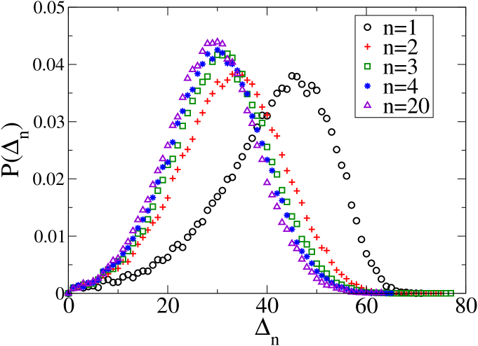
Figure 3: Distribution of $\Delta_{n}=t_{n}-t_{n-1}$ for various values of $n$. For small $n$, the distribution is close to a Gumbel and for large $n$, it evolves to a Gaussian. $w/(N\lambda)=10^{-2}$, $N=10^{6}$, $\lambda=0.1$.

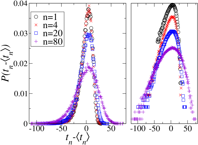
Figure 4: Distribution of $t_{n}$ for various values of $n$. The distribution remains close to Gumbel shapes even at large $n$. The plot on the right is in log-scale on the y-axis and the curves are shifted vertically for clarity. $w/(N\lambda)=10^{-2}$, $N=10^{6}$, $\lambda=0.1$.

General populations and weights

We now consider the general case of heterogeneous populations $N_{i}$ and fluxes $w_{i}$. The application of the same considerations as in the case of a homogeneous line leads to $\langle t_{n}\rangle=\sum_{i=1}^{n}\langle\Delta_{i}\rangle$. Since our main goal is to understand the case of complex networks which usually have the small-world property (i.e. a small diameter varying typically as $\log N$), we will now focus on the properties of $t_{n}$ at small $n$. Assuming that the average of $\Delta_{i}$ remains close to the formula for the arrival time in the first city ($\langle\Delta_{i}\rangle\approx\langle t_{1}(\lambda,w_{i},N_{i})\rangle$), we obtain

$$\lambda\langle t_{n}\rangle\approx\chi_{n}\equiv\ln\left[\prod_{i=0}^{n-1}\frac{N_{i}\lambda e^{-\gamma}}{w_{i}}\right]\ .$$ (11)

This expression links the expected arrival time in city $n$ of a stochastic spreading event to the quantity $\chi_{n}$ which depends on the properties of the line on which the spreading propagates. It is symmetric by permutations of weights and populations, and Figure 5 shows in fact that the whole distribution of arrival times, obtained through numerical simulations of the discrete stochastic dynamics, and not only its average, respects this symmetry. In the numerical simulations, heterogeneous populations and travel fluxes are uniformly distributed ($w_{i}\in[10,2000]$ and $N_{i}\in[10^{5},2.10^{7}]$). Figure 5 shows that the distribution of arrival times is invariant when one replaces (i) all the random weights by their geometrical mean $\overline{w}=(\prod_{i=0\dots n}w_{i})^{1/n}$; (ii) all the random populations by their geometrical mean $\overline{N}=(\prod_{i=0\dots n}N_{i})^{1/n}$; (iii) all weights by $\overline{w}$ and all populations by $\overline{N}$. The ratios of the average arrival times for these different sets $\langle t(\{w_{i}\},\{N_{i}\})\rangle/\langle t(\overline{w},\{N_{i}\})\rangle$, $\langle t(\{w_{i}\},\{N_{i}\})\rangle/\langle t(\{w_{i}\},\overline{N})\rangle$ and $\langle t(\{w_{i}\},\{N_{i}\})\rangle/\langle t(\bar{w},\bar{N})\rangle$ stay very close to $1$, with deviations at most of the order of $5\%$.

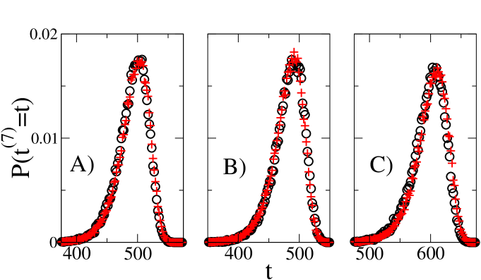
Figure 5: (A-C) Black circles indicate the arrival time distribution on a line at the city $\#$7 obtained for a fixed random set of populations $\{N_{i}\}$ and weights $\{w_{i}\}$ ($3$ different sets are used in the $3$ graphs). Red crosses correspond to the same distribution obtained A) with uniform travel $w_{i}=\bar{w}$, and populations $\{N_{i}\}$; B) with uniform populations $N_{i}=\bar{N}$, and weights $\{w_{i}\}$; C) with uniform populations $N_{i}=\bar{N}$ and uniform weights $w_{i}=\bar{w}$.

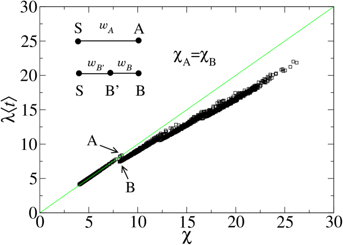
Figure 6: $\lambda\langle t\rangle$ vs $\chi$ for $5$ cities connected on a line. Each point correspond to the average arrival time in one of the city of the line, for one realization of the weights $w$, averaged over $10^{3}$ realizations of the epidemic spread. Results are presented for $100$ different random sets $\{w_{i}\}$.

We test in Fig. 6 the relation (11) which predicts the average arrival time measured in numerical simulations of the stochastic model. We use for simplicity uniform populations $N=10^{6}$, and we measure, for each fixed set of weights, the arrival time in each city, averaged over $10^{3}$ stochastic realizations of the spread. Figure 6 displays $\lambda\langle t_{i}\rangle$ versus $\chi_{i}$ for the various cities of a $5$ cities line, for $100$ different random sets of weights (each point corresponds to one given set of weights). We first note that $\lambda\langle t_{i}\rangle$ is a monotonous function of $\chi_{i}$. The figure also clearly shows that $\chi$ systematically overestimates the average arrival time. This is due, as already explained in the discussion of Eq. (9), to the fact that the use of $\langle\Delta\rangle_{Gumbel}$ neglects correlations, and in particular the travel between cities $n-2$ and $n-1$ for the estimate of the arrival time in $n$. Since this travel term increases $I_{n-1}$, it increases the probability that an infectious travels from $n-1$ to $n$, and therefore reduces $t_{n}$. This overestimation effect is not present for the first group of points that lie on the diagonal of the figure and correspond to cities directly connected to the seed. For this first group of cities, the average arrival time is indeed correctly given by $\chi$. On the other hand, the small overestimation can already be observed for cities at distance $2$ of the seed. For example, points $A$ and $B$ highlighted in Fig. 6 have the same $\chi_{B}=\chi_{A}=\chi$. Point $A$ corresponds to a city directly connected to the seed $S$, with a flux of $w_{A}$ passengers per unit time, such that $\chi_{A}=\ln(N\lambda/w_{A})-\gamma$, while point $B$ is obtained for a city which lies at topological distance two from the seed, with a city $B^{\prime}$ in between and such that $\chi_{B}=\ln\left(\frac{N\lambda}{w_{B}e^{\gamma}}\right)+\ln\left(\frac{N\lambda}{w_{B^{\prime}}e^{\gamma}}\right)$. The two cases correspond to the same value of $\chi$, but to different average arrival times: the arrival time in $B$ is smaller than in $A$, even if $\chi_{A}=\chi_{B}$, because relation (11) neglects the travel of additional infectious individuals between $S$ and $B^{\prime}$ to compute $\langle t_{B}\rangle$. Despite this systematic effect, Fig. 6 shows that relation (11) allows to define a quantity which depends only of the populations and passenger fluxes, and such that the average arrival time of the spreading is a monotonous function of this quantity. In the following, we will investigate how to generalize this quantity to more complex topologies.

3.3 From the one-dimensional line to complex networks

Equation (11) gives an estimate of the average arrival time in a city $n$ connected to the seed of the spreading through links with certain fluxes, and corresponds to a sum of the quantity $\ln(N\lambda/w)-\gamma$ along the links followed by the disease from the seed to city $n$. In a network, the sum can be computed along any of the paths linking the seed $s$ to any other city $j$. Since these different paths correspond a priori to different fluxes and to different arrival times, a natural approach consists in approximating the average arrival time in $j$, starting from a given seed $s$, by the minimum of (11) over all possible paths:

$$\lambda\langle t_{j}\rangle\approx\chi\left(j|s\right)\equiv\min_{\{P_{s,j}\}}\sum_{\left(k,l\right)\in P_{s,j}}\left[\ln\left(\frac{N_{k}\lambda}{w_{kl}}\right)-\gamma\right]$$ (12)

where $s$ is the seed, $\{P_{s,j}\}$ is the set of all possible paths connecting $s$ to $j$, and the sum is performed over the links $\left(k,l\right)$ along each path. In other terms, we have introduced a new weight on each oriented link $\left(k,l\right)$ of the network: $\ln\left(\frac{N_{k}\lambda}{w_{kl}}\right)-\gamma$. The quantity $\chi\left(j|s\right)$ is then the weighted distance between the seed $s$ and the node $j$ on this non-symmetric network (such a quantity can easily be computed for any topology using the Dijkstra algorithm (Dijkstra,, 1959)). Note that since the weights are real-valued, it is highly improbable that two different paths with the same sum of weights exist, so that equation (12) selects a unique path between $s$ and $j$.

Differences between propagation on a one-dimensional line and on a network can be expected from the two following important topological differences between these structures: (i) paths go through nodes with degree larger than $2$ and (ii) there are usually more than one path between two points. We first focus on the effect of the intermediate nodes with possibly large degrees through which the disease propagates. To this aim, we consider the simple topology consisting of a node $0$ connected to $k$ neighbors (as shown in the inset of Fig. 7). The infectious individuals, when they arrive at the central node, have multiple possible travel destinations. The probability for each destination to become infected is thus decreased; if the seed is in $0$ for instance, the initial infectious individual may even travel to a different peripherical node before creating an endogenous epidemic growth in the hub. This effect can be quantified by measuring the average arrival time of the disease in a given peripheral city $i$ in various situations. We first consider the case of a spreading phenomenon starting in a randomly chosen peripheral node, $i_{0}\neq i$, and compare the average arrival time in $i$ with the average arrival time in the one-dimensional situation in which only cities $i_{0}$, $0$ and $i$ are present. The ratio of these two times is displayed in Fig. 7 (‘seed: not hub’) as a function of the degree $k$ of the central node. We also show in the same figure the ratio of arrival times when the seed is $0$, i.e. the hub itself (”seed: hub”), and the topology is either the one of the inset, or the simple two-cities configuration in which only $0$ and $i$ are present and connected. In all cases, the arrival time in $i$ is increased by the presence of other possible connections from the hub. The effect is stronger for larger degree when the seed is the hub itself. The multiplicity of possible destinations therefore not only decreases the predictability of the spread (Colizza et al., 2006a, ), but also increases the average disease arrival time in a given city.

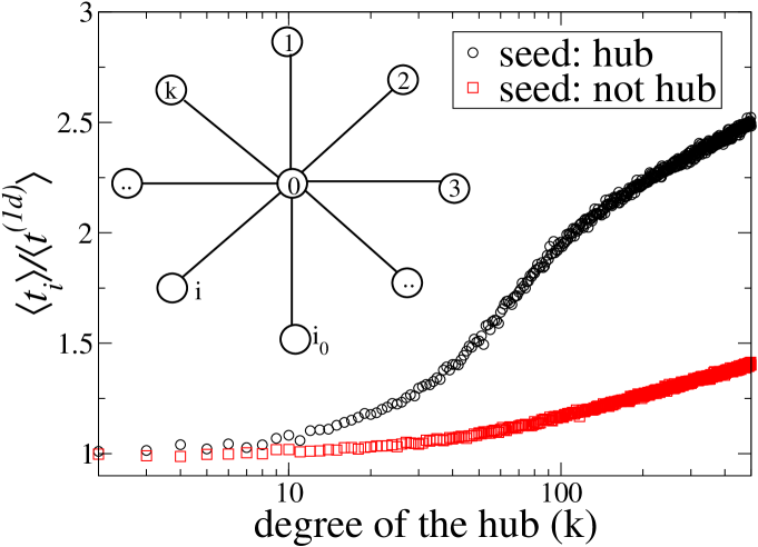
Figure 7: Ratio $\langle t_{i}\rangle/\langle t_{i}^{(1d)}\rangle$ of the average arrival time in a fixed peripheral city $i$ of the network shown in the inset and the average arrival time in the $1d$ case, vs the degree of the hub, $k$. Averages are done over $1000$ realizations of the spreading, with parameter $\frac{w}{N\lambda}=10^{-2}$. Circles: the seed is the hub; squares: the seed is one of the peripheral cities.

Another important point distinguishes a propagation in a network from a one dimensional line: namely, that multiple paths can often be found between two given nodes. In fact, it has already been shown by Crépey et al., (2006) in the case in which nodes represent individuals and not subpopulations, that the average arrival time is decreased by the presence of multiple paths, and that not only the shortest paths contribute to the spread between the seed and other nodes. To quantify this effect in metapopulation models, we consider the simple topology depicted in Fig. 8: a node $A$ (population $N_{A}$) is connected to a node $B$ by two different paths of length two. The first path connects $A$ with weight $w_{1}$ to an intermediate city $C$ of population $N$, which is in its turn connected to $B$ with weight $w_{2}$. The second path has weights $w^{\prime}_{1}$ and $w^{\prime}_{2}$, and the intermediate city $C^{\prime}$ has population $N^{\prime}$. We denote the probability that the disease spread reaches the city $B$ at time $t$ by $P\left(t\right)$ if the two paths are present, by $P_{ACB}\left(t\right)$ if only the first path through $C$ (weights $w_{1}$, $w_{2}$) is present, and by $P_{AC^{\prime}B}\left(t\right)$ if only the second path (through $C^{\prime}$, weights $w^{\prime}_{1}$, $w^{\prime}_{2}$) is present. Since the epidemics reaches $B$ from $A$ through one path or the other, $P(t)$ can be expressed as

$$P\left(t\right)=\left(1-\int_{0}^{t}P_{ACB}\left(\tau\right)d\tau\right)P_{AC^{\prime}B}\left(t\right)+\left(1-\int_{0}^{t}P_{AC^{\prime}B}\left(\tau\right)d\tau\right)P_{ACB}\left(t\right)$$ (13)

The data shown in Fig. 4 suggest that we can assume that $P_{ACB}$ and $P_{AC^{\prime}B}$ are Gumbel distributions, of averages $\chi_{ACB}=\ln\left(\frac{N_{A}\lambda}{w_{1}}\right)+\ln\left(\frac{N\lambda}{w_{2}}\right)-2\gamma$ and $\chi_{AC^{\prime}B}=\ln\left(\frac{N_{A}\lambda}{w^{\prime}_{1}}\right)+\ln\left(\frac{N^{\prime}\lambda}{w^{\prime}_{2}}\right)-2\gamma$, respectively. We introduce the quantities $w_{eq}=\frac{w_{1}w_{2}e^{\gamma}}{N\lambda}$ and $w^{\prime}_{eq}=\frac{w^{\prime}_{1}w^{\prime}_{2}e^{\gamma}}{N^{\prime}\lambda}$. The quantity $w_{eq}$ can be seen as the travel flux which, if $A$ and $B$ were directly connected, would yield the same arrival time distribution than the real two links $AC$ and $CB$ with weights $w_{1}$ and $w_{2}$: $\chi_{ACB}=\ln\left(\frac{N_{A}\lambda}{w_{eq}}\right)-\gamma$. We then have

$$P_{ACB}\left(t\right)=\frac{w_{eq}}{N_{A}}e^{\lambda t-\frac{w_{eq}}{N_{A}\lambda}e^{\lambda t}}$$ (14)

$$P_{AC^{\prime}B}\left(t\right)=\frac{w^{\prime}_{eq}}{N_{A}}e^{\lambda t-\frac{w^{\prime}_{eq}}{N_{A}\lambda}e^{\lambda t}}$$ (15)

and finally from Eq. (13) (using the fact that the weights are small with respect to the quantities $N\lambda$, $N^{\prime}\lambda$, $N_{A}\lambda$)

$$P\left(t\right)=\frac{w_{eq}+w^{\prime}_{eq}}{N_{A}}\exp\left(\lambda t-\frac{w_{eq}+w^{\prime}_{eq}}{N_{A}\lambda}e^{\lambda t}\right)\ .$$ (16)

We note that $P(t)$ is also a Gumbel distribution, and the average of the arrival time in $B$, $\langle t_{mp}\rangle$ (mp=multiple paths), can be easily calculated:

$$\lambda\langle t_{mp}\rangle=\chi_{mp}\equiv\ln\left(\frac{N_{A}\lambda}{w_{eq}+w^{\prime}_{eq}}\right)-\gamma\ ,$$ (17)

so that the existence of two paths results in the law

$$e^{-\chi_{mp}}=e^{-\chi_{ACB}}+e^{-\chi_{AC^{\prime}B}}\ .$$ (18)

We have checked this prediction by numerical simulations of stochastic spreading in the small network formed by nodes $A$, $B$, $C$ and $C^{\prime}$, in the simple case of $N_{A}=N=N^{\prime}$ and $w_{1}=w_{2}\equiv w$, $w^{\prime}_{1}=w^{\prime}_{2}\equiv w^{\prime}$. Figure 8 displays the ratio of the average arrival time in $B$, for a spread seeded in $A$, to the average arrival time in $B$ when only one path (the one with weights $w$) is present. We consider only $w^{\prime}\leq w$ since the situation with $w^{\prime}\geq w$ is obtained by exchanging the two paths. As $w^{\prime}\to 0$, this ratio goes to $1$, while, in the other extreme case $w^{\prime}\to w$, a decrease of the average arrival time close to $10\%$ is obtained. Moreover, the prediction (18), shown as continuous line, is in excellent agreement with the numerical data.

Interestingly, when more than two paths are present, Eq. (18) can easily be generalized to a sum over all possible paths (not necessarily of length $2$): $\lambda\langle t_{mp}\rangle=\chi_{mp}$ with

$$e^{-\chi_{mp}}=\sum_{paths}e^{-\chi_{path}}\ ,$$ (19)

where $\chi_{path}$ is computed on each path by Eq. (11). Figure 9 presents a comparison of numerical results with this analytical prediction, for various path multiplicities, showing a very good agreement. Similar results are obtained for paths of larger lengths.

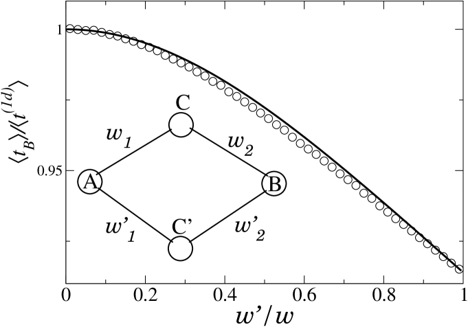
Figure 8: Ratio of the average arrival time in $B$ (the seed is $A$) and the average arrival time in the $1d$ case (when only the path $ACB$ is connected), versus $w^{\prime}/w$ (in the simulations $w_{1}=w_{2}=w$, $w^{\prime}_{1}=w^{\prime}_{2}=w^{\prime}$, and $N=N^{\prime}=N_{A}$). Averages are done over $1,000$ realizations of the spreading, with $w=10^{3}$ and $\frac{w}{N\lambda}=10^{-2}$. All cities have the same population $N=10^{6}$. Full line: theoretical prediction (17).

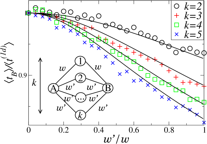
Figure 9: Ratio of the average arrival time in $B$ (the seed is $A$ with degree $k$) to the average arrival time in the $1d$ case (when only the path $A1B$ is connected), vs $w^{\prime}/w$. Averages are done over $1,000$ realizations of the spread, with $w=10^{3}$ and $\frac{w}{N\lambda}=10^{-2}$. All cities have the same population, $N=10^{6}$. Numerical results (symbols) are compared to the theoretical model given by Eq. (19) (full lines) for different values of $k$.

We have also investigated numerically, on simple topologies but with random weights, how well the average arrival time in a city is correlated with $\chi_{mp}$ computed as in (19). In particular, Fig. 10 displays the average arrival time in city $B$, connected to the seed $A$ of the spreading by $k$ paths of length $l$ and random weights, as a function of both $\chi_{B}$ given by Eq. (12) (i.e. computed along the path that minimizes $\chi$) and $\chi_{mp}$ which takes into account all paths. While $\chi_{mp}$ is slightly more strongly correlated with $\langle t\rangle$ than $\chi_{B}$, and closer to its actual value, the improvement is not striking. We have also developed an algorithm to compute $\chi_{mp}$ on a complex network, by taking into account the contributions of all paths of topological lengths $d$ and $d+1$ (where $d$ is the length of the shortest path, in terms of topology, between the seed and the considered city). While the algorithmic complexity is increased (we used techniques based on the Brandes algorithm (Brandes,, 2001)) with respect to the computation of (12), the obtained improvement was again significative but not striking.

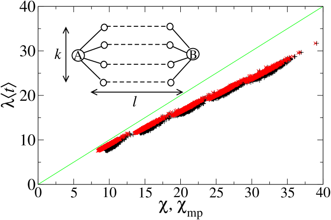
Figure 10: Correlations between the average time $\langle t\rangle$ of arrival in $B$ and $\chi\left(B\right)$ (black), and between $\langle t\rangle$ and $\chi_{mp}\left(B\right)$ (red), for the network represented in the inset. The different points correspond to different values of $k$ (from $2$ to $5$), different path lengths $l$ (from $2$ to $6$) and different realizations of the disorder of the links ($100$ different sets of $\{w\}$ for each structure). Averages are done over $1,000$ realizations of the spreading.

4 The world-wide airport network

We now proceed to numerical simulations of the metapopulation model on the Worldwide airport network, which displays various levels of complexity and heterogeneity (Barrat et al.,, 2004; Guimerà et al.,, 2005; Colizza et al., 2006a, ; Colizza et al., 2006b, ). At the topological level, the degree distribution is broad and can be approximated by a power-law; the links’ weights (fluxes) are also broadly distributed and span several orders of magnitude. Finally, the world city populations are also broadly distributed according to Zipf’s law (Zipf,, 1949). All these heterogeneity levels have been shown to play relevant roles in the spread of epidemics at the worldwide level (Colizza et al., 2006a, ; Colizza et al., 2006b, ). We perform the numerical simulations of the stochastic spreading on the network containing the $2,400$ largest airports, which takes into account $98\%$ of the total traffic (the WAN comprises $3,100$ airports, but we consider here only the links verifying $\ln\left(\frac{N\lambda}{w}\right)>0$, which amounts to the removal of the smallest airports; in particular, a certain number of nodes have a larger traffic than inhabitants, which leads to a local breakdown of the relation between $p_{ij}$ and the local population and travel flow).

4.1 Average arrival time

Figure 11 displays the average arrival time in the various cities, $\lambda\langle t_{i}\rangle$, as a function of $\chi_{i}$ as defined by (12). For each given seed, averages are done over $1,000$ stochastic realizations of the disease spread. The figure clearly shows that the value of $\chi$ determines the average arrival time (the two quantities are very strongly correlated) and various cities with the same $\chi$ are reached at the same time by the propagation. As in the case of the simple topologies studied above, $\chi$ in fact systematically overestimates the correct average arrival time, but can still be considered as a very good approximation.

Figure 11 also highlights the effect of hubs, analyzed in the previous section. Frankfurt is indeed the node with the largest degree in the network, and the arrival times at a given value of $\chi$ is larger than for other seeds with a smaller degree. This effect remains however quite small and is essentially limited to the first reached cities. The arrival times seem to be closer to our Ansatz. This stems from the delay introduced by the large degree of the initial seed, as discussed in the previous section, which increases all the arrival times, therefore slightly shifting the data upwards and partially compensating for the fact that $\chi$ overestimates these times. We finally note how very similar results are obtained for the SIR model. As expected, the important time scale in the SIR (as well as in the SIS) is $\lambda-\mu$: this quantity controls the endogenous growth of the epidemic at small times. We have investigated a wide range of values for $\lambda-\mu$, as well as for $\lambda$ in the simple SI case. The arrival time is well determined by $\chi$ as long as the condition $w/N\lambda<<1$ given in section 3 is satisfied.

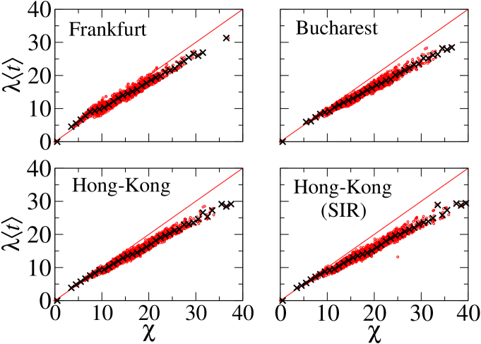
Figure 11: $\lambda\langle t\rangle$ versus $\chi$ on the WAN for diseases starting in different cities. Each red dot corresponds to a city and averages are done over $1,000$ realizations of the spread. Crosses are an average over cities with the same $\chi$. The starting seeds are Frankfurt (degree $240$), Bucharest (degree $56$) and Hong-Kong (degree $109$). When the initial seed is a hub, the average arrival time is larger, especially in the first reached cities, due to the effect of the degree. We also show $\lambda\langle t\rangle$ versus $\chi$ for a SIR model seeded in Hong-Kong.

Figure 11 conveys the result that the average arrival times are not exactly given by $\chi$, but are at least determined to a large extent, given a seed, by this quantity. An immediate application of this result is given by a possible prediction of the order of arrival of the disease in different cities. In order to compare the list of cities ranked by the average arrival time and the same list ordered according to $\chi$, we compute the indicator known as Kendall’s $\tau$. This indicator allows a quantitative analysis of the correlations between two rankings of $n$ objects (Numerical Recipes,, 2004) and is given by

$$\tau=\frac{n_{c}-n_{d}}{n(n-1)/2}$$ (20)

where $n_{c}$ is the number of pairs whose order does not change in the two different lists and $n_{d}$ is the number of pairs whose order is inverted. This quantity is normalized between $-1$ and $1$: $\tau=1$ corresponds to identical rankings while $\tau=0$ is the average for two uncorrelated rankings, and $\tau=-1$ is a perfect anticorrelation.

We present in the first column of Table 1 the values of $\tau$ for the lists of cities ordered according respectively to the average arrival time of the spread and to the values of $\chi$, for various seeds. The second column of the table gives the values of $\tau$ when the lists are ordered by average arrival time and by $\chi_{mp}$. In both cases the values are extremely high (two random permutations of a list of size $N=2,400$ would give an indicator normally distributed with mean $0$ and variance $\frac{4N+10}{9N(N-1)}=2.10^{-4}$ (Numerical Recipes,, 2004)). In order to better emphasize this strong correlation between the ordered list, we also display in Table 1 the $\tau$ of Kendall between the city list ordered by average arrival time and by different distances from the propagation seed. As noted in the introduction, the topological distance $d$ from the seed is not completely irrelevant, but other weighted distances which take into account the diversity of fluxes and populations could be expected to be more strongly correlated with the arrival time. In particular, a first possibility consists in defining the effective ”length” of each edge as the inverse of the weight, $\ell_{ij}=1/w_{ij}$: the disease will spread more easily on an edge if many passengers travel across it. The corresponding weighted distance between nodes on the network is noted $d_{1/w}$. Since the ratios $N/w$ moreover appear naturally in the travel probabilities, we also consider that a directed length $N_{i}/w_{ij}$ can be defined on each edge, and the distance between each node and the seed can as well be computed ($d_{N/w}$). The results indicate significant correlations between the average arrival times and these various distances. The correlations are however much stronger with $\chi$ and $\chi_{mp}$, showing that these quantities can be used with a good confidence as an estimate of the average arrival time order. Very similar results are obtained for SIS or SIR models, with respectively $\tau_{SIS}\{\langle t\rangle,\chi\}\approx 0.875$ and $\tau_{SIR}\{\langle t\rangle,\chi\}\approx 0.866$, for a spreading process seeded in Hong-Kong.

Seed	$\{\langle t\rangle,\chi\}$	$\{\langle t\rangle,\chi_{mp}\}$	$\{\langle t\rangle,d\}$	$\{\langle t\rangle,d_{N/w}\}$	$\{\langle t\rangle,d_{1/w}\}$
FRA	0.856	0.917	0.299	0.311	0.3
HKG	0.874	0.934	0.212	0.275	0.262
OTP	0.866	0.938	0.301	0.304	0.284
SJK	0.883	0.906	0.292	0.287	0.275

Table 1: Kendall’s $\tau$ for the list of cities ranked by arrival order and the list obtained with different indicators. Each line corresponds to a different seed: Frankfurt (FRA, degree $240$), Hong-Kong (HKG, degree $109$). Bucharest (OTP, degree $56$) and Sao Jose dos Campos (SJK, Brazil, degree $6$).

4.2 Arrival order for a given realization

The previous results are valid for the average arrival times, and it is legitimate to ask about their relevance to the case of a single spreading event. Indeed, in the real-world there is not such a thing as averages over different realizations. The natural extension of our results therefore consists in checking if the quantity $\chi$ can predict the order in which the disease will reach the various nodes (cities) of the network in each stochastic realization of the spread. More precisely we can compute, for each pair of nodes $(i,j)$ in the network, and for a given infection seed, the probability that the arrival times in $i$ and $j$ for the same realization of the spread, $t_{i}$ and $t_{j}$, are correctly ordered by their values of $\chi$, i.e. that they verify $(t_{i}-t_{j})(\chi_{i}-\chi_{j})>0$. We use the notation $\Delta\chi\left(i,j\right)=\mid\chi_{j}-\chi_{i}\mid$ and Fig. 12 displays the probability $f_{c}$ that a couple of nodes with a $\chi$-difference $\Delta\chi\left(i,j\right)=\Delta\chi$ are reached by the disease in the order predicted by their values of $\chi$. If $\Delta\chi\left(i,j\right)=0$, no prediction can be made and we obtain indeed $f_{c}=0.5$. On the other hand, if $\Delta\chi(i,j)$ is large ($>10$), the two nodes are reached in the correctly predicted order in every realization of the spread.

Since not all node pairs have very different values of $\chi$ (and thus a large value of $\Delta\chi$), we also show as in Fig. 12 the cumulative distribution $p_{>}(\Delta\chi)$ of the number of couples of nodes with a given value of $\Delta\chi$. For instance, for a spreading process seeded in Hong-Kong (degree $109$), $75\%$ of the couples have $\Delta\chi>2$, and these pairs are correctly sorted with a probability larger than $80\%$, instead of only $50\%$ on average if no information is available. Figure 12 moreover shows that the precision is higher when the seed has a small degree. On the other hand, if the seed is Frankfurt (of degree $240$, data not shown), the situation is slightly worsened, as can be expected from the smaller global predictability of the spread starting from a hub (Colizza et al., 2006a, ), due to the many possible travel destinations available for the infectious individuals. In this case, $80\%$ of the couples have $\Delta\chi>2$, and these pairs are correctly sorted with a probability larger than $70\%$; the probability $f_{c}$ is larger than $90\%$ for $47\%$ of the pairs. Similar results are obtained when the endogenous growth of the disease is described by SIS or SIR models.

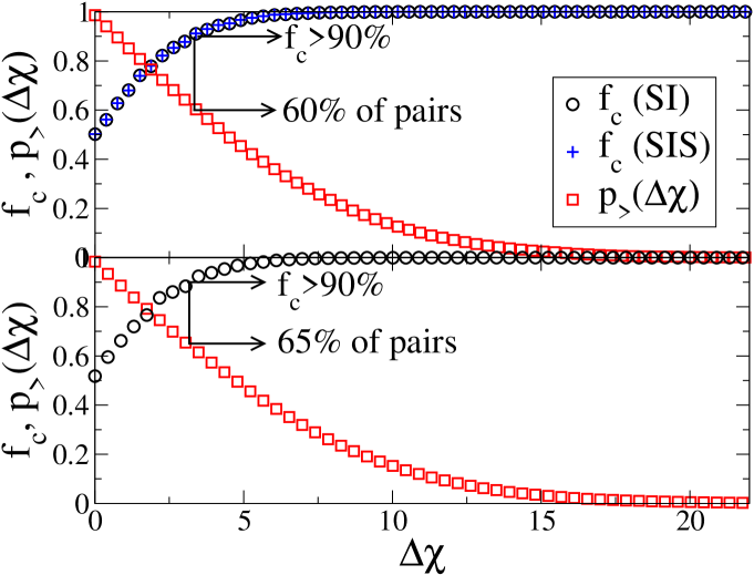
Figure 12: Fraction of couples of nodes correctly ranked as a function of their $\Delta\chi$ (circles), in each realization of the spread, and cumulative distribution (squares) of the values of $\Delta\chi$ (i.e., fraction of couples of cities $(i,j)$ with $\Delta\chi(i,j)=\mid\chi\left(j\right)-\chi\left(i\right)\mid>\Delta\chi$). Top: the seed is Hong-Kong, a node of degree $109$, and the curves of $f_{c}$ for both SI (circles) and SIR (crosses) processes are shown. Bottom: the seed has degree $6$ (Sao Jose dos Campos, Brazil).

We also present in Fig. 13 the same quantities $f_{c}$ and $p_{>}(\Delta\chi)$ for couples of nodes having the same topological distance from the seed. While this topological distance is indeed too simple a quantity to be really useful in the prediction of arrival times, it can seem reasonable that a node at distance $1$ from the seed will anyway be reached before a node at distance $5$. If large values of $\Delta\chi$ were obtained only for nodes at very different topological distances from the seed, the prediction shown in Fig. 12 would not be particularly relevant. We see in Fig. 13 that nodes at the same topological distance from the seed can have very different values of $\chi$ and be therefore reached by the disease in an order which can be almost certainly predicted by measuring their values of $\chi$. For example, Fig. 13 shows that more than $70\%$ of the couples are well ranked with a probability larger than $70\%$, even if the two nodes are at the same topological distance ($d=2$, $3$, $4$ or $5$) from the seed. Results are presented for a seed with large degree, and slightly better results are obtained for smaller degree seeds.

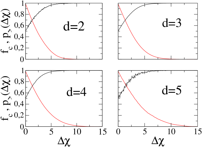
Figure 13: Same quantities as in Fig. 12, but each graph concerns only couples of nodes at the same topological distance from the seed, $d$. From top left to bottom right : $d=2$, $d=3$, $d=4$ and $d=5$. The seed is Frankfurt (degree $240$).

Finally, another quantitative indication of the relevance of the quantity $\chi$ is obtained, similarly to the previous subsection, by comparing the list of cities ordered either by $\chi$ or by the arrival time of the spread in a given realization (and not the average arrival time as in the previous section). Kendall’s $\tau$ is therefore now a quantity which fluctuates from one realization to the other (for a given seed), and the corresponding histograms are shown, for various seeds, in Fig. 14. The values obtained are systematically larger than $0.5$, denoting a strong correlation between the lists ordered according to the arrival time and $\chi$. Moreover, the figure highlights how seeds with larger degrees lead to smaller values of $\tau$. This is in agreement with the slightly better prediction capacities displayed in Fig. 12 when the seed has small degree. Interestingly, this result can also be related to the issue of predictability studied by Colizza et al., 2006a ; Colizza et al., 2006b : the predictability of a spreading process, as measured by the similarity between two stochastic realizations with the same initial conditions, has indeed been shown to be larger when the seed has a small degree.

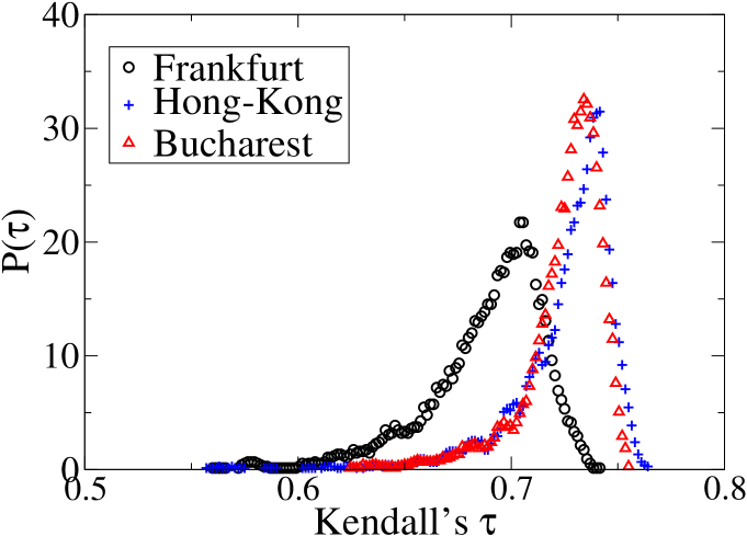
Figure 14: Histogram of Kendall’s $\tau$ for the list of cities sorted according either to the arrival time in a given realization or to $\chi$. Different seeds yield different histograms.

5 Conclusion

In this paper, we have studied a metapopulation model for the spread of epidemics on a large scale in which subpopulations (cities) are linked by fluxes of passengers. Such models are particularly useful for the analysis of epidemics which propagate worldwide along the airline connections (Rvachev & Longini,, 1985; Hufnagel et al.,, 2004; Colizza et al., 2006a, ; Colizza et al., 2006b, ; Colizza et al., 2007a, ). They couple endogenous evolutions of epidemics inside each subpopulation with diffusion along the network of connections, which opens interesting new perspectives (Colizza et al., 2007b, ). In this study, we have focused on the issue of arrival times of epidemics, as a function of the seed and of the network’s characteristics. We have proposed a quantity easily computable on any network which depends only on the links weights and nodes populations, and which accounts for the average arrival time of the spread in each city. This quantity allows to sort the various subpopulations according to the order of arrival of each single realization of the spread with a very good accuracy. We note that this quantity is given by a certain weighted distance computed on a directed weighted graph, and in particular that this distance selects a shortest weighted path between the seed and the various nodes. This result could therefore shed some light on the existence and properties of “epidemic pathways” whose relevant role was already suggested by Colizza et al., 2006a ; Colizza et al., 2006b and which certainly deserve further work. In particular, the role and relative importance of the multiple paths should be investigated. These predictive tools could play an important role in the set-up of containment measures and policies. It would also be interesting to adapt the proposed quantity to more refined or sophisticated compartmental models (Elveback et al.,, 1976; Watts et al.,, 2005), or to generalize it to different scales such as the urban scale, where nodes are places like home, work or malls (Eubank et al.,, 2004).

6 Acknowledgments

It is a pleasure to thank Vittoria Colizza and Alessandro Vespignani for discussions. A.G. and M.B. also thank the School of Informatics, Indiana University where part of this work was performed. We are particularly grateful to Vittoria Colizza for sharing with us the data on the city populations and we also thank IATA (http://www.iata.org) for making their database available to us. A.G. and A.B. are partially supported by the EU under contract 001907 (DELIS).

References

- Albert & Barabási, (2002) Albert, R. & Barabási, A.-L. (2002). Statistical mechanics of complex networks. Rev. Mod. Phys. 74, 47–97.
- Anderson & May, (1992) Anderson, R. M. & May, R. M. (1992). Infectious diseases in humans. Oxford: Oxford University Press.
- Baroyan et al., (1969) Baroyan, O.V., Genchikov, L.A., Rvachev, L.A. & Shashkov, V.A. (1969). An attempt at large-scale influenza epidemic modelling by means of a computer. Bull. Internat. Epidemiol. Assoc., 18, 22-31.
- Barrat et al., (2004) Barrat, A., Barthélemy, M., Pastor-Satorras, R. & Vespignani, A. (2004). The architecture of complex weighted networks. Proc. Natl. Acad. Sci. USA, 101, 3747–3752.
- Barthélemy et al., (2005) Barthélemy, M., Barrat, A., Pastor-Satorras, R. & Vespignani, A. (2005). Dynamical patterns of epidemic outbreaks in complex heterogeneous networks. J. Theor. Bio. 235, 275.
- Boccaletti et al., (2006) Boccaletti, S., Latora, V., Moreno, Y., Chavez, M. & Wang, D.-U. (2006) Complex networks: structure and dynamics. Phys. Rep. 424, 175.
- Brandes, (2001) Brandes, U. (2001) A Faster Algorithm for Betweenness Centrality. J. math. sociol. 25, 163-177.
- Brownstein et al., (2006) Brownstein, J.S., Wolfe, C.J. & Mandl, K.D. (2006) Empirical Evidence for the Effect of Airline Travel on Inter-Regional Influenza Spread in the United States. PLoS 3, e401.
- Chowell et al., (2003) Chowell, G., Hyman, J.M., Eubank, S. & Castillo-Chavez, C. (2003), Scaling laws for the movement of people between locations in a large city Phys. Rev. E 68, 066102.
- Cliff & Haggett, (2004) Cliff, A. & Haggett, P. (2004). Time, travel and infection. British Medical Bulletin, 69. 87-99.
- Cohen, (2000) Cohen, M.L. (2000). Changing patterns of infectious disease. Nature 406, 762-767.
- (12) Colizza, V., Barrat, A., Barthélemy, M. & Vespignani A. (2006a). The role of the airline transportation network in the prediction and predictability of global epidemics. Proc. Natl. Acad. Sci. USA 103, 2015-2020.
- (13) Colizza, V., Barrat, A., Barthélemy, M. & Vespignani A. (2006b). The modeling of global epidemics: stochastic dynamics and predictability Bull. Math. Biol. 68, 1893 (2006).
- (14) Colizza, V., Barrat, A., Barthélemy, M. & Vespignani A. (2007a) Modeling the world-wide spread of pandemic influenza: baseline case and containment interventions PLoS Medicine 4, e13.
- (15) Colizza, V., Pastor-Satorras, R. & Vespignani, A. (2007b). Reaction-diffusion processes and meta-population models in heterogeneous networks. Nature Physics 3, 276-282.
- Colizza & Vespignani, (2007) Colizza, V., & Vespignani, A. (2007). Epidemic modeling in metapopulation systems with heterogeneous coupling pattern: theory and simulations. preprint arXiv:0706.3647.
- Crépey et al., (2006) Crépey, P., Alvarez, F.P., & Barthelemy, M. (2006). Epidemic variability in complex networks. Phys Rev E 73, 046131.
- Dijkstra, (1959) Dijkstra, E.W. (1959). A note on two problems in connexion with graphs. Numerische Mathematik 1, 83-89.
- Dorogovtsev & Mendes, (2003) Dorogovtsev, S. N. & Mendes, J. F. F. (2003). Evolution of networks: From biological nets to the Internet and WWW. Oxford: Oxford University Press.
- Elveback et al., (1976) Elveback, L.R., Fox, J.P., Ackerman, E., Langworthy, A., Boyd, M. & Gatewood, L. (1976). An influenza simulation model for immunization studies. Am J epidemiol 103, 152-165.
- Eubank et al., (2004) Eubank, S., Guclu, H., Kumar, A., Marathe, M. V., Srinivasan, A., Toroczkai, Z. & Wang, N. (2004). Modelling disease outbreaks in realistic urban social networks. Nature, 429, 180–184.
- Ferguson et al., (2003) Ferguson, N. M., Keeling, M. J., Edmunds, W. J., Gani, R., Greenfell, B. T. & Anderson, R. M. (2003). Planning for smallpox outbreaks. Nature, 425, 681–685.
- Flahault & Valleron, (1992) Flahault, A. & Valleron, A.-J. (1992). A method for assessing the global spread of HIV-1 infection based on air-travel Math. Popul. Stud. 3, 161-171.
- Gautreau et al., (2007) Gautreau, A. Barrat, A., & Barthélemy, M. (2007), Arrival Time Statistics in Global Disease Spread. J. Stat. Mech. L09001.
- Grais et al., (2003) Grais, R.F., Hugh Ellis, J., & Glass, G.E. (2003), Assessing the impact of airline travel on the geographic spread of pandemic influenza. European Journal of Epidemiology 18, 1065-1072.
- Guimerà et al., (2005) Guimerà, R., Mossa, S., Turtschi, A. & Amaral, L.A.N. (2005). The worldwide air transportation network: Anomalous centrality, community structure, and cities’ global roles. Proc. Natl. Acad. Sci. USA 102, 7794..
- Hethcote & Yorke, (1984) Hethcote, H. W. & Yorke, J. A. (1984). Gonorrhea: transmission and control. Lect. Notes Biomath. 56, 1–105.
- Hufnagel et al., (2004) Hufnagel, L., Brockmann, D. & Geisel, T. (2004). Forecast and control of epidemics in a globalized world. Proc. Natl. Acad. Sci. (USA) 101, 15124-15129.
- Keeling, (1999) Keeling, M. (1999). The Effects of Local Spatial Structure on Epidemiological Invasions. Proc. R. Soc. Lond. B 266, 859-867.
- Kretzschmar & Morris, (1996) Kretzschmar, M. & Morris, M. (1996). Measures of concurrency in networks and the spread of infectious disease. Math. Biosci. 133, 165-195.
- Longini, (1988) Longini, I.M. (1988). A mathematical model for predicting the geographic spread of new infectious agents. Mathematical Biosciences 90, 367-383.
- May & Lloyd (2001) May, R. M. & Lloyd, A. L. (2001). Infection dynamics on scale-free networks. Phys. Rev. E 64, 066112.
- Meyers et al., (2005) Meyers, L.A, Pourbohloul B., Newman, M.E.J., Skowronski, D.M. & Brunham,R.C. (2005). Network theory and SARS: predicting outbreak diversity. Journal of Theor. Biol. 232 71-81.
- Murray, (2004) Murray, J.D. (2004). Mathematical Biology II. 3rd edition, Springer.
- Noh & Rieger, (2003) Noh, J. D. & Rieger, H. (2004) Random Walks on Complex Networks. Phys. Rev. Lett. 92, 118701.
- Numerical Recipes, (2004) Numerical Recipes (2004). Numerical Recipes in C : the Art of Scientific Computing. Cambridge University Press.
- (37) Pastor-Satorras, R. & Vespignani, A. (2001a). Epidemic spreading in scale-free networks. Phys. Rev. Lett. 86, 3200–3203.
- (38) Pastor-Satorras, R. & Vespignani, A. (2001b). Epidemic dynamics and endemic states in complex networks. Phys. Rev. E, 63, 066117.
- Pastor-Satorras & Vespignani, (2004) Pastor-Satorras, R. & Vespignani, A. (2004). Evolution and structure of the Internet: A statistical physics approach. Cambridge: Cambridge University Press.
- Rvachev & Longini, (1985) Rvachev, L.A. & Longini, I.M. (1985). A mathematical model for the global spread of influenza. Mathematical Biosciences 75, 3-22.
- Watts et al., (2005) Watts, D.J., Muhamad, R., Medina, D.C. & Dodds, P.S. (2005). Multiscale, resurgent epidemics in a hierarchical metapopulation model. Proc. Natl. Acad. Sci. USA 102, 11157-11162.
- Wu et al., (2006) Wu, Z., Braunstein, L. A., Colizza, V., Cohen, R., Havlin, S. & Stanley, H. E. (2006). Optimal paths in complex networks with correlated weights: The worldwide airport network. Phys. Rev. E 74, 056104.
- Zipf, (1949) Zipf, G. K. (1949). Human behavior and the principle of least effort. Addison-Wesley Press Cambridge, Massachussets.