Magnetoconductance of interacting electrons in quantum wires: Spin density functional theory study

Abstract

We present systematic quantitative description of the magnetoconductance of split-gate quantum wires focusing on formation and evolution of the odd (spin-resolved) conductance plateaus. We start from the case of spinless electrons where the calculated magnetoconductance in the Hartree approximation shows the plateaus quantized in units of 2$e^{2}/h$ separated by transition regions whose width grows as the magnetic field is increased. We show that the transition regions are related to the formation of the compressible strips in the middle of the wire occupied by electrons belonging to the highest (spin-degenerate) subband. Accounting for the exchange and correlation interactions within the spin density functional theory (DFT) leads to lifting of the spin degeneracy and formation of the spin-resolved plateaus at odd values of $e^{2}/h.$ The most striking feature of the magnetoconductance is that the width of the odd conductance steps in the spin DFT calculations is equal to the width of the transition intervals between the conductance steps in the Hartree calculations. A detailed analysis of the evolution of the Hartree and the spin-DFT subband structure provides an explanation of this finding. Our calculations also reveal the effect of the collapse of the odd conductance plateaus for lower fields. We attribute this effect to the reduced screening efficiency in the confined (wire) geometry when the width of the compressible strip in the center becomes much smaller than the extend of the wave function. A detailed comparison to the experimental data demonstrates that the spin-DFT calculations reproduce not only qualitatively, but rather quantitatively all the features observed in the experiment. This includes the dependence of the width of the odd and even plateaus on the magnetic field as well as the estimation of the subband index corresponding to the last resolved odd plateau in the magnetoconductance.

I Introduction

The quantized conductance of a two-dimensional electron gas (2DEG) in the quantum Hall regime has generated a tremendous attention since its discovery in 1980vonKlitzing . For a theoretical description of the integer quantum Hall (IQH) effect, the concept of edge states combined with the Landauer-Buttiker formalism is widely usededges ; BvH . This approach is proved to be especially appealing for the description of electron transport in the quantum Hall regime in confined geometries like quantum wires or quantum point contacts (QPCs)vanWees ; BvH .

Some aspects of the quantized conductance in the confined geometries in the IQH regime can be understood in a one-electron picture. This includes, for example, magnetic depopulation of the subbands in a quantum wireBerggren , and selective population and detection of edge channels by QPCs resulting in the observation of anomalous IQH effectvanWees ; BvH . In the one-electron picture the two-terminal magnetoconductance $G$ of a quantum wire or a QPC exhibits quantized plateaus in units of $2e^{2}/h$ (for spinless electrons) separated by transition regions of an essentially zero width. The experiments, however, show that an extend of these transition regions can be comparable to the width of the plateausBvH ; vanWees ; Wrobel ; experiment . This indicates that an accurate description of the magnetoconductance in the IQH regime even without accounting for spin effects requires approaches that go beyond a simple one-electron picture of non-interacting electrons. A quantitative electrostatic theory of interacting electrons in quantum wires was proposed by Chklovskii, Matveev and ShklovskiiChklovskiiII . They demonstrated that in a strong magnetic field, alternating strips of compressible and incompressible liquids are formed in the center of the wire. They also evaluated the two-terminal magnetoconductance of the wire. In contrast to the one-electron description, the magnetoconductance of interacting electron was shown to exhibits very narrow quantized plateaus separated by much broader rises where the conductance was not quantized. This conclusion (being opposite to the prediction of the one-electron picture) is also in apparent disagreement with the experiments. This indicates that even for spinless electrons in the IQH regime an accurate quantitative description of the magnetoconductance requires many-body quantum mechanical treatment.

At low temperature in clean high-mobility samples the spin degeneracy is lifted and the additional plateaus at odd values of $e^{2}/h$ become resolvedBvH ; experiment . This is due to the exchange and correlations effects leading to the strong enhancement of the electron $g$ factor above its bulk valueUemura . The effect of the many-body interactions on the spin splitting in quantum wires in the IQH regime has been a subject of numerous studiesKinaret ; Dempsey ; Tokura ; Manolescu ; Takis ; Takis2 ; Stoof ; Kramer ; Studart ; Ihnatsenka ; Ihnatsenka2 ; Ihnatsenka3 ; hysteresis ; HF . These studies have focused on various aspects of 2DEG in confined geometries including the structure of compressible/incompressible strips, suppression or enhancement of the $g$ factor, subband spin splitting, spatial spin separation and other. We however have not been able to find in the literature any systematic quantitative treatment of the magnetoconductance of the structures at hand. Surprisingly enough, even after two decades of the studies of IQH systems in the confined geometry, the question of the fundamental importance addressing the formation of the odd plateaus in the magnetoconductance and corresponding quantitative description of the plateau widths still remains unanswered. As discussed above, the structure of the magnetoconductance plateaus remains poorly understood even for the case of spinless electrons. Recent advances in the field such as demonstration of the Mach–ZehnderJi , Aharonov-BohmGoldman_AB , and Laughlin quasiparticle interferometersGoldman or prospects of the topological quantum computingTopQuantComp has led to a renewed interested to the magnetoconductance in the quantum wires and related structures. Even though many of the the above systems operate in the fractional quantum Hall regime where the correlation effects become dominant, a detailed understanding of the magnetoconductance in the IQH regime is the necessary prerequisite for the understanding of the magnetotransport in the fractional regime.

In our previous publications we provided a systematic quantitative description of the structure and spin polarization of edge states and magnetosubband evolution in the quantum wire based on the self-consistent Green’s function techniques combined with the spin density functional theory (DFT)Ihnatsenka ; Ihnatsenka2 ; Ihnatsenka3 or Hartree-Fock approachHF . The main aim of this paper is to present a systematic quantitative description of the two-terminal magnetonductance of the quantum wire with the focus on the formation and evolution of the exchange-induced odd conductance plateaus. The motivation for the present paper is the recent experimental studies of the spin-resolved magnetoconductance of the narrow channels in the IQH regimeexperiment . One of the remarkable finding of this experiment is the collapse of the spin splitting in the confined geometries for lower field. The spin-DFT magnetotransport calculations presented in this paper not only capture essential features observed in the experiment, but demonstrate rather good quantitative agreement with the calculated and observed magnetoconductances. This includes the width and the position of the magnetoconductance plateaus (both odd and even), as well as predictions for the critical magnetic field where the odd plateaus disappear in the magnetoconductance. We therefore conclude that the spin DFT approach represents the powerful tool to study large realistic quantum Hall systems containing hundreds or thousands of electrons, providing detailed and reliable microscopic information on wavefunctions, electron densities and currents as well as the conductance.

II Basics

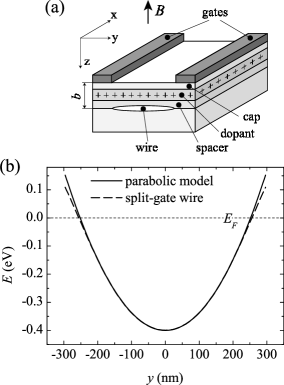
Figure 1: (a) Schematic diagram of a split-gate quantum wire. (b) The bare electrostatic parabolic confining potential $V_{conf}(y)$ (Eq. (1)) with $V_{0}=-0.4$ eV, $\hbar\omega_{0}=3.8$ meV (solid lines). Dashed lines shows the calculated electrostatic confinement for a realistic split-gate quantum wires depicted in (a) with the distance between the gates $a=500$ nm, the gate voltage $V_{g}=-2$ V, $\delta-$donor concentration $n_{d}=6\cdot 10^{23}$ m^-3, the donor and electron distance to the surface are 100 nm and 200 nm respectively and the Schottky barrier $V_{Schottky}=0.8$ eV (The potentials from the gates and the donors are calculated on the basis of Eqs. (2) and (3) of Ref. Ihnatsenka, ).

We consider an infinitely long wire in a perpendicular magnetic field $B$, see Fig. 1. The bare electrostatic confinement (due to the split gates, the donor layer and the Schottky barrier) can be approximated by a parabolic potential,

$$V_{conf}(y)=V_{0}+\frac{m^{\ast}}{2}\left(\omega_{0}y\right)^{2},$$ (1)

where $V_{0}$ is the bottom of the potential, $\omega_{0}$ defines the potential slope, and $m^{\ast}=0.067m_{e}$ is the electron effective mass in GaAs. [The comparison of the model parabolic potential with the calculated potential in a realistic split gate wire is shown in Fig. 1(b)]. By varying $V_{0}$ and $\omega_{0}$ we can change the wire width and the electron density; in our calculations we set the Fermi energy $E_{F}=0$.

In order to calculate the magnetoconductance of the quantum wire, its subband structure and the wavefunctions we use the Green’s function techniqueIhnatsenka ; Ihnatsenka2 where the electron interaction and the spin effects are included self-consistently within the framework of the Kohn-Sham density function theory in the local spin density approximationGiuliani_Vignale . (The reliability of the the spin density functional theory for electronic structure and magnetotransport calculations in quantum wires, dots and related structures is discussed in details in Refs. HF, ; conductance, ).

We start from the Hamiltonian $H=\sum_{\sigma}\left(H_{0}+V^{\sigma}(y)\right),$ where $H_{0}$ is the kinetic energy in the Landau gauge,

$$H_{0}=-\frac{\hbar^{2}}{2m^{\ast}}\left\{\left(\frac{\partial}{\partial x}-\frac{eiBy}{\hbar}\right)^{2}+\frac{\partial^{2}}{\partial y^{2}}\right\},$$ (2)

and the total confining potential $V^{\sigma}(y),$

$$V^{\sigma}(y)=V_{conf}(y)+V_{H}(y)+V_{xc}^{\sigma}(y)+V_{Z}^{\sigma}$$ (3)

includes the bare electrostatic confinement $V_{conf}(y)$ (given by Eq. (1)), the Hartree potential $V_{H}(y),$ the exchange-correlation potential $V_{xc}^{\sigma}(y),$ and the Zeeman term, $V_{Z}^{\sigma}=g\mu_{b}B\sigma,$ where $\sigma=\pm\frac{1}{2}$ describes the spin-up and spin-down states, $\uparrow$ ,$\downarrow;$ $\mu_{b}=e\hbar/2m_{e}$ is the Bohr magneton, and the bulk $g$ factor of GaAs is $g=-0.44.$ The Hartree potential $V_{H}(y)$ due to the electron density $n(y)=\sum_{\sigma}n^{\sigma}(y)$ (including the mirror charges) readsIhnatsenka

$$V_{H}(y)=-\frac{e^{2}}{4\pi\varepsilon_{0}\varepsilon_{r}}\int_{-\infty}^{+\infty}dy^{\prime}n(y^{\prime})\ln\frac{\left(y-y^{\prime}\right)^{2}}{\left(y-y^{\prime}\right)^{2}+4b^{2}},$$ (4)

with $b$ being the distance from the electron gas to the surface (we choose $b=200$ nm). The exchange and correlation potential $V_{xc}(y)$ in the local spin density approximation is given by the functional derivative

$$V_{xc}^{\sigma}(y)=\frac{\delta}{\delta n^{\sigma}}\left\{n\epsilon_{xc}\left(n,\zeta(y)\right)\right\}$$ (5)

where $\zeta(y)=\frac{n^{\uparrow}-n^{\downarrow}}{n^{\uparrow}+n^{\downarrow}}$ is the local spin-polarization. In the present paper we use the parameterization of the exchange and correlation energy $\epsilon_{xc}$ given by Tanatar and Ceperly (TC)TC . Note that we also performed calculations on the basis of the parametrization recently provided by Attaccalite et al. AMGB and found only marginal difference with the results based on the TC functional.

The spin-resolved electron density in the wire can be expressed via the Green’s function $G^{\sigma}(y,y,E)$

$$n^{\sigma}(y)=-\frac{1}{\pi}\text{Im}\left[\int_{-\infty}^{\infty}dE\,G^{\sigma}(y,y,E)f_{FD}(E-E_{F})\right],$$ (6)

where $f_{FD}(E-E_{F})$ is the Fermi-Dirac distribution function. The Green’s function, the Bloch states, the electron and current densities are calculated self-consistently using the technique described in detail in Ref. [Ihnatsenka, ]. Knowledge of the wave vectors $k_{\alpha}^{\sigma}$ for different Bloch states $\alpha$ allows us to recover the subband structure, i.e. to calculate an overage position $y_{\alpha}^{\sigma}$ of the wave functions for different modes $\alpha$ for the given energy $E$ Davies_book ,

$$y_{\alpha}^{\sigma}=\frac{\hbar k_{\alpha}^{\sigma}}{eB}.$$ (7)

We calculate the spin-resolved conductance of the wire on the basis of the linear-response Landauer formula,

$$G^{\sigma}=\frac{e^{2}}{h}\sum_{\alpha}\int_{E_{th\,\alpha}^{\sigma}}^{\infty}dE\left(-\frac{\partial f\left(E-E_{F}\right)}{\partial E}\right),$$ (8)

where summation is performed over all propagating modes $\alpha$ for the spin $\sigma,$ with $E_{th\,\alpha}^{\sigma}$ being the propagation threshold for $\alpha$-th mode. The current density for a mode $\alpha$ is calculated as Ihnatsenka

$$J_{\alpha}^{\sigma}(y)=\frac{e^{2}}{h}V\int dE\frac{j_{\alpha}^{\sigma}(y,E)}{v_{\alpha}^{\sigma}}\left(-\frac{\partial f\left(E-E_{F}\right)}{\partial E}\right),$$ (9)

with $v_{\alpha}^{\sigma}$ and $j_{\alpha}^{\sigma}(y,E)$ being respectively the group velocity and the quantum-mechanical particle current density for the state $\alpha$ at the energy $E$, and $V$ being the applied voltage. All the calculations presented in this paper are performed for the temperature $T=100$ mK. In order to speed up the calculation we use the modified Broyden methodBroyden that allows one to reduce the number of iterations need to achieve a self-consistent solution from $\sim 2000$ to only $\sim 50$ .

III Result and discussions

III.1 Hartree and spin DFT approximations

We start our analysis of the magnetoconductance and the magnetosubband structure in quantum wires from the case of the Hartree approximation when the exchange and correlation interactions are not included in the effective potential (i.e. when $V_{xc}^{\sigma}(y)$ is set to zero in Eq. (3)). Note that the total potential $V^{\sigma}(y)$ also includes the Zeeman term leading to the spin splitting even in the Hartree case. The effect of the Zeeman term is however negligibly small in the considered field intervals. We will thus refer to the Hartree case as for the case of spinless electrons. The results obtained in the Hartree approximation will provide a basis for understanding of the effect of the exchange and correlation within the spin DFT approximation.

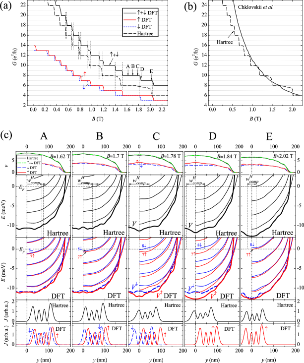
Figure 2: (a) Conductance of the quantum wire calculated within the spin DFT and in the Hartree approximation (the later is shifted by $-2e^{2}/h$ for clarity). The vertical lines are drawn to emphasize that the width of the odd conductance steps in the spin DFT calculations is equal to the width of the transition intervals between the conductance steps in the Hartree calculations. (b) Comparison of between the Hartree magnetoconductance and the magnetoconductance calculated according to the Chklovskii et al. conjecture $G_{Ch}=\frac{2e^{2}}{h}\nu(0)$. (c) Evolution of the magnetosubband structure in the interval $6e^{2}/h<G<8e^{2}/h$ (second and third row). Fat solid lines indicate the total confining potential. The first row shows the electron density profiles (local filling factors) $\nu(y)=n(y)/n_{B}$ $(n_{B}=eB/h)$. Two lower rows show the current densities for the last two subbands ($N=7,8$). Parameters of the wire are the same as in Fig. 1, $T=100$mK.

Figure 2(a),(b) shows the magnetoconductance of a representative wire with the effective width $w\approx 350$ nm and the electron density in the center of the wire $n(0)=3.2\cdot 10^{15}$ m^-2 calculated within the Hartree and the spin DFT approximations. The Hartree magnetoconductance shows the plateaus quantized in units of 2$e^{2}/h$ separated by transition regions whose width grows as the magnetic field is increased. For large fields the width of the transition regions is comparable or can even exceed the width of the neighboring plateaus. For low fields, $B\lesssim B_{\text{crit}},$ the width of the transition regions practically shrinks to zero; for the quantum wire at hand this critical field is $B_{\text{crit}}\sim 0.6$T, corresponding to the subband index $N\approx 17,$ see Fig. 2(a). Note that in a standard one-electron picture of edge states the magnetoconductance of a clean wire (without impurities) is strictly quantized in units of $2e^{2}/h$ (for spinless electrons), with vanishing width of the transition regions. Formation of the transition region between the plateaus is shown to be related to development of the compressible strip in the middle of the wireChklovskiiII .

Let us now turn to the spin-resolved magnetoconductance calculated by the spin DFT. The most striking feature of the wire magnetoconductance is that the width of the odd conductance steps in the spin DFT calculations is equal to the width of the transition intervals between the conductance steps in the Hartree calculations, see Fig. 2(a). We will demonstrate below that the characteristic features in the spin-resolved conductance of the quantum wires calculated on the basis of the spin DFT (including the dependence of the width of the odd plateaus on the magnetic field and collapse of the odd plateaus at lower fields $B\lesssim B_{\text{crit}}$) can be understood from the analysis of the compressible strip structure for spinless electrons and the corresponding magnetoconductance and the magnetosubband structure evolution in the Hartree approximation.

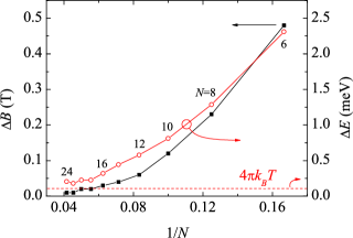
Figure 3: Solid line: The width of the transition regions between the Hartree plateaus (which is equal to the width of the odd plateaus in the spin DFT calculations) as a function of $1/N$, with $N$ being the subband number (indicated in the plot). Thin line: The subband splitting in the wire center $\Delta E=E$ (the definition of $\Delta E$ is illustrated in Fig. 4). Parameters of the wire are the same as in Fig. 1, $T=100$mK.

Before we proceed to the analysis of the evolution of the magnetosubband structure, it is instrumental to outline how the exchange interaction induces the spin splitting (see for details Refs. Ihnatsenka, ; Ihnatsenka2, ). The spin splitting is most pronounced in the compressible strips. Indeed, the Hartree compressible strips are formed for partially occupied states in the vicinity of $E_{F}$ when the Fermi-Dirac occupation $f_{FD}<1$ (i.e. in the window $|E-E_{F}|<2\pi kT$). When the states are partially occupied, the system behaves like a metal, where the electrons can easily readjust their density to screen the external potential. It is important to stress that the compressible strips, being partially occupied, allow for different population of the spin-up and spin-down states. In the DFT calculations, this population difference (triggered by the Zeeman splitting) is strongly enhanced by the exchange interaction. This leads to the lifting of the subband degeneracy and to the spatial separation between the spin-up and spin-down states.

III.2 The magnetosubband structure and the magnetoconductance

In order to get insight into evolution of the odd conductance plateaus let us inspect the Hartree and the spin DFT magnetosubband structure. Let us, for example, concentrate at the field region where $6e^{2}/h<G<8e^{2}/h$, i.e. when the magnetoconductance clearly shows the spin splitting. The magnetosubband structure for several representative fields in this region is shown in Fig. 2(c). In all subsequent discussions we will focus on the two highest subbands (in this case $N=8$ and $N=7$), because the depopulation of these two subbands determines the features in the conductance steps (note that all the remaining subbands are fully filled). At $B=1.62$T the subbands $N=7,8$ are fully occupied and thus the total conductance $G=8e^{2}/h$. The Hartree calculations for spinless electrons show the presence of a narrow compressible strip of the width $w_{comp}^{H}$, see Fig. 2 A. When the exchange interaction is included, the subbands split which leads to the spatial separation between the spin-up and spin-down states. (The spatial spin separation due to the suppression of the Hartree compressible strips was discussed in detail in Ref. Ihnatsenka2, ).

When magnetic field is increased the subbands are pushed up in energy (see Fig. 2 B; $B=1.7$T). The compressible strip in the Hartree calculations becomes wider (because the confinement is smoother in the wire center), and it moves closer to the center of the wire. The exchange interaction quenches the compressible strip causing the splitting of the spin-up and spin-down subbands. However, despite of the lifting of the spin degeneracy the subband bottoms are still below $E_{F}$ at the wire center. Because of this, the two spin split subbands $N=7,8$ remain fully (and equally) populated and the conductance remains on the plateau $G=8e^{2}/h$.

When the magnetic field is increased to $B=1.78$T (Fig. 2 C), the Hartree compressible strip reaches the middle of the wire. This means that the subbands become partially occupied because their bottoms are now within the window $|E-E_{F}|<2\pi kT$ (where $f_{FD}<1$). As a result, the conductance of the spinless Hartree electrons starts to decrease and the transition region between the plateaus starts to form. With further increase of the magnetic field the Hartree compressible strip in the middle of the wire shrinks, and at $B\approx 2.05$T the subbands depopulate completely, as they are pushed above the window $|E-E_{F}|=2\pi kT$. We conclude the discussion of the evolution of the Hartree subbands by re-emphasizing the fact that the transition between the conductance steps starts when the compressible strip reaches the center of the wire and it ends when the compressible strip disappears and two highest (spin-degenerate) magnetosubband are pushed above $E_{F}$. Note that even though this discussion was focused on the transition between $G=8e^{2}/h$ and $6e^{2}/h$-plateaus in the Hartree conductance, the same scenario of the Hartree subband depopulation holds for all other subbands.

Let us now examine how the exchange interaction affects the transition region between the Hartree plateaus $G=8e^{2}/h$ and $6e^{2}/h$. Similarly to the cases of lower fields discussed above (Fig. 2 A, B), the exchange interaction causes the subband repulsion and the spatial spin separation of the wavefunctions (the latter being equal to the width of the Hartree compressible strips, see the lower panel of Fig. 2(c)). For $B=1.78$T the Hartree compressible strip covers the central part of the wire. As a result, the bottom of the higher energy (spin-down $N=8$) subband is situated within the window $|E-E_{F}|<2\pi kT$ (and thus this subband is only partially populated), whereas $N=7$ (spin-down) subband is pushed below $E_{F}$ and thus remains fully populated (Fig. 4 C, spin DFT calculations). Thus, at $B=1.78$T the transition to the odd plateau $G=7e^{2}/h$ starts to form. The exchange interaction keeps 8th and 7th subbands separated such that with further increase of the magnetic field 8th subband becomes quickly depopulated while 7th subband remains fully occupied with its bottom being below $E_{F}$, see Fig. 4 D, E ($B=1.84$T and $B=2.05$T). The above field interval (i.e. $1.84\text{T}<B<2.05$T) corresponds to the odd step in the magnetoconductance. Finally, at $B=2.05$T (i.e. at the same field when the corresponding Hartree subbands depopulate), the bottom of 7th subband is pushed above $E_{F}$ (to be more precise, above $E_{F}+2\pi kT$) and 7th plateau in the conductance disappears.

To summarize the discussion presented in this section, the formation of the odd magnetoconductance plateaus due to the exchange interaction can be traced to the formation of the compressible strips in the center of the wire in the case of the spinless electrons. The exchange interaction lifts the spin degeneracy such that the bottom of the highest (even) subband remains pinned to $E_{F}$, whereas the bottom of the highest odd subband remains below $E_{E}$. As a result, the odd plateaus (whose width is equal to the width of the transition regions between the Hartree plateaus) develop in the magnetoconductance.

Note that the analytical solution to the electrostatic problem of the electron density distribution in a quantum wire for spinless electrons has been obtained by Chklovskii, Matveev and Shklovski ChklovskiiII for the high magnetic field regime (when only a few lower Landau levels are occupied, $N\lesssim 2\sim 4$). [A good agreement with with the analytical results of Chklovskii et al. has been reported by Oh and Gerhardts within the self-consistent Thomas-Fermi calculations Oh ]. Chklovskii et al.ChklovskiiII have also discussed the magnetoconductance of the quantum wire. They found that in a realistic quantum wire the conductance plateaus are practically absent, i.e. the conductance is not quantized (see Fig. 5 in Ref. ChklovskiiII, ). This conclusion is in obvious disagreement with the experimental results showing pronounced plateaus in the two-terminal magnetoconductance at integer values of $e^{2}/h.$ BvH ; Wrobel ; experiment . They attributed this discrepancy to the presence of disorder in the channel. We however, have demonstrated above that even in an ideal clean channel (without disorder) the conductance shows the pronounced quantization with wide plateaus and sharp rises. The reason of the discrepancy we instead attribute to the conjecture used by Chklovskiet al. that the ballistic conductance is given by the filling factor in the middle of the wire, $G_{Ch}=\frac{2e^{2}}{h}\nu(0)$. Our quantum mechanical calculations show that this conjecture is not justified. Indeed, the comparison of the conductance calculated according to the Chklovskii et al. conjecture with the magnetoconductance calculated according to Eq. (8) (see Fig. 2(b)) shows that $G_{Ch}$ reproduces the overall decrease of the conductance rather well, but does not at all recover the steps in the conductance related to the subband depopulation (see also Ref. Lier, for a related discussion). Our results thus indicate that while electrostatic and Thomas-Fermi-type approaches can be very successful in the description of the electron density and the structure of the compressible and incompressible strips for the spinless electrons, an accurate description of the magnetoconductance requires detailed quantum mechanical information for the wave functions and the currents densities.

III.3 Collapse of the odd magnetoconductance plateaus at lower fields

When magnetic field is increased, the width of the transition regions between the Hartree plateaus (which is equal to the width of the odd plateaus in the spin resolved magnetoconductance), $\Delta B$, is also gradually increases, see Figs 2,3. We attribute this increase of $\Delta B$ to the effect of the enhanced electron screening due to the evolution of the compressible strip in the middle of the wire. Indeed, the transition regions between the Hartree plateaus are related to the depopulation of the highest (spin-degenerate) subbands forming the compressible strip in the center. In high magnetic field each subband (representing a Landau level) accommodates the same number of electrons, such that the density of the electrons in the highest subband is proportional to $\sim 1/N$. Thus, one can expect that the width of the compressible strip in the middle of the wire $w_{comp}$ and hence the width $\Delta B$ grow as $B$ increases (note that $B\sim 1/N)$. Figures 3 - 5 illustrating the magnetic field dependence of $\Delta B$ and $w_{comp}$ confirms this expectation. Note that $\Delta B$ shows a nonlinear dependence on $1/N$. That is, for low fields, $B\lesssim B_{\text{crit}},$ the width $\Delta B$ rapidly decreases when $B$ decreases, such that the odd plateaus are no longer seen in the magnetoconductance.

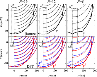
Figure 4: The magnetosubband structure of a quantum wire within the Hartree and the spin-DFT approximation for different number of occupied subbands $N$. Fat solid lines indicate the total confining potential. [For all cases the magnetic field is chosen such that the Hartree compressible strips in the middle of the wire have a maximal width]. $\Delta E$ shows the subband splitting in the center of the wire. Parameters of the wire are the same as in Fig. 1, $T=100$mK.

Let us now concentrate on this feature of magnetoconductance in more detail. Figure 2 shows the spin-resolved magnetoconductance $G^{\uparrow}$ and $G^{\downarrow}$ . It is worth to stress that the spin degeneracy remains lifted even for fields smaller than $B_{crit}$. The total conductance $G=G^{\uparrow}+G^{\downarrow}$ does not however exhibits the odd plateaus for $B<B_{crit}$ because the strength of the exchange splitting becomes comparable to the thermal broadening of the plateaus. This is illustrated in Fig. 3 that shows the dependence of the subband splitting $\Delta E$ in the center of the wire on the magnetic field and its comparison to the energy window $4\pi kT$ (where the derivative of the Fermi-Dirac distribution function is distinct from zero). [The definition of the subband splitting $\Delta E$ is outlined in Fig. 4]. It is also worth pointing out that in accordance to the previous discussion, $\Delta E$ and $\Delta B$ exhibit similar behavior as a function of magnetic field, see Fig. 3.

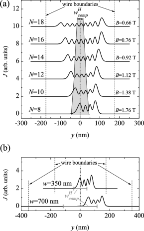
Figure 5: (a) The current densities for the highest occupied Hartree subband compared to the maximal width of the compressible strip in the middle of the wire for different magnetic fields. $N$ indicates the subband number (see Fig. 4 for the corresponding magnetosubband structure). (b)The current densities for the highest occupied Hartree subband ($N=8$) compared to the maximal width of the compressible strip in the wires with the effective widths of $w=350$ nm and $w=700$ nm. Parameters of the wire are the same as in Fig. 1, parameters of the second wire are indicated in Fig. 6; $T=100$mK.

In order to understand the nonlinear behavior of $\Delta B$ leading to quenching of the odd magnetoconductance plateaus at low field we examine the wave functions and the current density distributions. Figure 5 (a) shows the current density for the Hartree subbands $N=8-18$ along with the maximal width of the Hartree compressible strip $w_{comp}$ in the middle of the wire. The extend of the wave function for the highest $N$th subband, $\langle\psi_{N}\rangle\sim\sqrt{N}l_{B},$ ($l_{B}$ is the magnetic length) gradually increases when the magnetic field is loweredDavies_book . Note that $\langle\psi_{N}\rangle$ is larger than the width of the compressible strip $w_{comp}$ already for $N=8$. When the extend of the wave function exceeds the width of the compressible strip, the ability of the system to screen the external potential is greatly reduced because the wave function can be shifted within the distance not exceeding the width of the compressible strip $w_{comp}$. Thus, the smaller the ratio $w_{comp}/\langle\psi_{N}\rangle$ is, the weaker is the effect of the redistribution of the electron density required to screen the external potential. This reduced screening efficiency for lower fields (when $w_{comp}/\langle\psi_{N}\rangle\ll 1)$ translates into the suppressed exchange splitting and thus to disappearance of the odd magnetoconductance plateaus.

Note that the extend of the wave function $\langle\psi_{N}\rangle$ for a given subband number $N$ (or for a given magnetic field) is not particularly sensitive to the wire width $w$ (at least in the regime when the cyclotron radius $r_{c}<w$). At the same time, the maximum width of the compressible strip increases with increase of the wire width. This is illustrated in Fig. 5(b) that shows the current density distribution and $w_{comp}$ for two quantum wires of the with $w=350$ nm and $700$ nm for the case of $N=6$ occupied subbands. [Note that in the bulk limit (i.e. for the edge of the 2DEG) the compressible strip covers the semi-infinite space, such that regardless of the subband number, $w_{comp}/\langle\psi_{N}\rangle\gg 1$]. Therefore, for the given $N$ (or magnetic field $B$) the ratio $w_{comp}/\langle\psi_{N}\rangle$ is larger in a wider wire and therefore the screening efficiency is higher. One can therefore expect that in a wider wire the magnetosubband spin splitting due to exchange interaction leading to the appearance of the odd magnetoconductance plateaus would manifest itself for larger subband numbers (lower fields). Our calculations show that this is indeed the case. For example, in a wire with $w=350$ nm the odd plateaus become discernible for the subband index $N=17$ ($B_{\text{crit}}\sim 0.6$T), whereas for the wire with $w=700$ nm the last odd plateau is seen for $N\sim 19-21$ ($B_{\text{crit}}\sim 0.4$T), c.f. Figs. 2 and 6

IV Comparison to the experiment

We have performed magnetotransport calculations for several quantum wires with effective widths in the range 200-700 nm and the electron densities $1.5-3.5\cdot 10^{15}$m${}^{-2}.$ All the wires exhibit the same behavior described in detail in previous section.

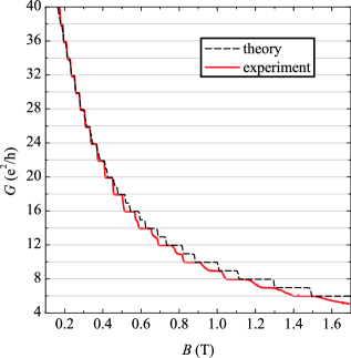
Figure 6: Comparison between the calculated magnetoconductance of the wire with the effective width of $w=700$nm and the experimental magnetoconductanceexperiment . $T=100$mK.

A detailed comparison of our calculations with the experimental magnetoconductanceexperiment for a some representative quantum wire is shown in Fig. 6. The width of the wire is estimated to be $\sim 680$ nm, and the sheet electron density in the bulk $n_{s}=2.15\cdot 10^{15}$m^-2.experiment . The theoretical magnetoconductance shown in Fig. 6 is calculated for the electrostatic confining potential with the parameters $V_{0}=-0.4$ eV, $\hbar\omega_{0}=1.91$ meV (giving the effective wire width $w=700$ nm and the electron density in the wire center $n=2.2\cdot 10^{15}$m^-2). In the both experimental and simulated wires the electrons is situated at the distance $\sim 200$ nm below the surface. The comparison to the subband depopulation in the experimental structure demonstrates that such a choice of the parameters provides a satisfactory approximation for the actual confining potential. We stress here that a magnetic field dependence of the subband depopulation can be described by the one-particle Schrödinger equation (for a given confining potential)Berggren , whereas our main focus here is the electron interaction effects leading to formation of the odd steps in the magnetoconductance due to the exchange interaction. The comparison of the calculated and the experimental curves demonstrates a good quantitative agreement between the widths of the odd (as well as even) plateaus in the calculated and the experimental magnetoconductance. The calculations also provide a reasonably close estimation of the subband index corresponding to the last resolved odd plateau in the magnetoconductance, $N\sim 19-21$, whereas the corresponding experimental value is $N=15.$

It would be unreasonable to expect an exact agreement between the theory and the experiment. There are several factors that have not been taken into account in the theoretical modelling. We list below some of them.

(a) The experimentexperiment is performed in the QPC geometry whereas our calculations are done for an infinite quantum wire. In the edge state transport regime considered here with $N\gg 1$ this is not expected to be a source of significant discrepancy between the theoretical predictions and the experiment. Nevertheless, the effect of the QPC geometry on the magnetoconductance remains to be seen.

(b) The calculations are performed for ideal clean wires without impurities. In a one electron description the transition regions between the magnetoconductance plateaus are the step functions with a zero width. A random impurity potential is known to lead to the smooth transition regions of a finite width even in the one-electron pictureAndo_1994 . A comparison of the magnetoconductance traces in Fig. 6 clearly shows that the the transition regions seen in the experiment are significantly wider than the theoretical ones. [We remind that a finite width of the transition regions in the theoretical magnetoconductance is due to the formation of the compressible strips in the middle of the wire]. We attribute the difference in the widths of the calculated and experimental transition regions to the effect of the disorder that has not been included in the model. Note the experimental magnetoconductance traces for narrower QPCs show the conductance fluctuations in the transition regionsexperiment , which is a clear manifestation of the disorder potential due to impuritiesdisorder . Note that the presence of disorder can also lead to the destruction of the exchange enhancement of the $g$-factor and thus to the collapse of the spin splitting (i.e. to the suppression of the odd plateaus for $N>N_{c}$)Fogler . This effect does not seem to be relevant to the experiment because the spin splitting, being suppressed in the narrow structures (QPCs) for larger $N$, is still clearly seen in the bulk Hall measurements.

(c) In our calculations we assumed that an electron motion is confined to a two-dimensional plane, which is a good approximation for heterostructures where the electrons are localized on the interface between GaAs/AlGaAs. In the experimental structuresexperiment the electrons are confined in a quantum well that is populated by donors situated on both sides from the well. An accurate description of this geometry might require accounting in the Schrödinger equation the electron motion in the direction perpendicular to the interface.

Finally, we notice that while we compared our calculations with the experimental conductance of one representative wire, our spin-DFT calculations qualitatively reproduce all the features observed in other samples. This includes the dependence of of the width of the odd plateaus $\Delta B$ on the magnetic field shown in Fig. 3. It is also worth to stress that the theory confirms (and explains) the experimental finding that in wider wires the collapse of the odd plateaus occurs at lower fields. We however are not in position to fit all the experimental data. This is because that this task would require a detailed knowledge of the bare confining electrostatic potential $V_{conf}$ due to the gates and the donor layers, Eq. (1). Indeed, the bare electrostatic confinement determines the total self-consistent confining potential $V^{\sigma}(y)$, which, in turn, determines the depopulation of the magnetosubbands (i.e. the dependence of the subband number $N$ on $B$)BvH ; Berggren . We are not in a position to perform a systematic search for the parameters of $V_{conf}$ giving rise to the $B$-dependence of the subband depopulation consistent with each experimental magnetoconductance trace. This is simply because of a computation burden related to this task: each point on the magnetoconductance plot requires up to one hour of a processor time. [Note that a calculation of the electrostatic confinement and the self-consistent potential starting from the layout of the actual heterostructure of Ref. experiment, represents a separate task which is outside a scope of the present study].

V Conclusion

In this paper we provide a systematic quantitative description of the magnetoconductance of the split-gate quantum wires focusing on the formation and evolution of the odd conductance plateaus. In order to calculate the electron density, magnetosubband structure and the magnetoconductance we utilize the self-consistent Greens function technique combined with the spin density functional theoryIhnatsenka .

We start our analysis with the case of spinless electrons in the Hartree approximation (disregarding the exchange and correlation interactions). The calculated Hartree magnetoconductance shows the plateaus quantized in units of 2$e^{2}/h$ separated by transition regions whose width grows as the magnetic field is increased. The transition regions are attributed to the formation of the compressible strips in the middle of the wire occupied by electrons belonging to the highest (spin-degenerate) subband. In agreement with experiments, the width of the transition regions for large fields is comparable to the width of the neighboring plateaus. This is in contrast to both the one-electron description where the conductance shows the step-like behavior with the rises between the plateaus of zero width, as well as to the electrostatic theory of Chklovskii et al.ChklovskiiII where the magnetoconductance exhibits narrow plateaus of negligible width separated by much broader transition regions where the conductance is not quantized.

Accounting for the exchange and correlation interactions within the spin DFT leads to the lifting of the spin degeneracy and formation of the spin-resolved plateaus at odd values of $e^{2}/h.$ The most striking feature of the magnetoconductance is that the width of the odd conductance steps in the spin DFT calculation is equal to the width of the transition intervals between the conductance steps in the Hartree calculations. This is because the transition intervals in the Hartree magnetoconductance correspond to the formation of the compressible strip in the middle of the wire. At the same time, in the compressible strip in the center of the wire the states are only partially occupied. As a result, the exchange interaction enhances the difference in the spin-up and spin-down population, which leads to the lifting of the subband spin degeneracy and formation of the odd conductance plateaus.

In agrement with the experimental resultsexperiment , we find that the width of the odd magnetoconductance plateaus gradually decreases with decrease of the magnetic field. For lower fields $B<B_{\text{crit}}$, the odd plateaus rapidly disappear such that the magnetoconductance shows the quantization in units of $2e^{2}/h.$ The wider the wire, the lower the critical field $B_{\text{crit}}$ corresponding to the disappearance of the last resolved odd plateau. We attribute this effect to the reduced screening efficiency in the confined (wire) geometry when the width of the compressible strip in the center becomes much smaller than the extend of the wave function. This, in turn, leads to the suppressed exchange splitting and collapse of the odd magnetoconductance steps.

A detailed comparison to the experimental dataexperiment (see Fig. 6) demonstrates that the spin-DFT calculations reproduce not only qualitatively, but rather quantitatively all the features observed in experiment. This includes the dependence of the width of the odd and even plateaus on the magnetic field as well as the estimation of the subband index corresponding to the last resolved odd plateau in the magnetoconductance. The experiment however shows wider rises between the transitions plateaus in comparison to the calculated ones. We attribute this difference to the effect of smooth potential due to remote donors that has not been accounted for in our calculations (performed for clean disorder-free wires). Despite of this discrepancy, the overall good agreement between the theory and experiment makes it possible to conclude that the spin DFT approach represents the powerful tool to study large realistic quantum Hall systems containing hundreds or thousands of electrons, providing detailed and reliable microscopic information on wavefunctions, electron densities and currents as well as the conductance.

- (1) K. v.Klitzing, G. Dorda, and M. Pepper, Phys. Rev. Lett. 45, 494 (1980).
- (2) B. I. Halperin, Phys. Rev. B 25, 2185 (1982); P. Streda, J. Kucera, and A. H. MacDonald, Phys. Rev. Lett. 59, 1973 (1987).
- (3) C. W. J. Beenakker and H. van Houten, Quantum Transport in Semiconductor Nanostructures, in Solid State Physics 44, 1 (1991).
- (4) B. J. van Wees, L. P. Kouwenhoven, E. M. M. Willems, C. J. P. M. Harmans, J. E. Mooij, H. van Houten, C. W. J. Beenakker, J. G. Williamson, and C. T. Foxon, Phys. Rev. B 43, 12431 (1991).
- (5) K.-F. Berggren, T. J. Thornton, D. J. Newson, and M. Pepper, Phys, Rev. Lett. 57, 1769 (1986).
- (6) J. Wrobel, T. Dietl, K. Reginski, and M. Bugajski, Phys. Rev. B 58, 16252 (1998)
- (7) I. P. Radu, J. B. Miller, S. Amasha, E. Levenson-Falk, D. M. Zumbuhl, M. A. Kastner, C. M. Marcus, L. N. Pfeiffer, and K. W. West, unpublished. (The layout and geometry of the devices and heterostructures are similar to those studied in J. B. Miller, I. P. Radu, D. M. Zumbuhl, E. Levenson-Falk, M. A. Kastner, C. M. Marcus, L. N. Pfeiffer, and K. W. West, Nature Physics 3, 561 (2007)).
- (8) D. B. Chklovskii, K. A. Matveev, and B. I. Shklovskii, Phys. Rev. B 47, 12605 (1993).
- (9) T. Ando and Y. Uemura, J. Phys. Soc. Jpn. 37, 1044 (1974).
- (10) J. M. Kinaret and P. A. Lee, Phys. Rev. B 42 11768 (1990).
- (11) J. Dempsey, B. Y. Gelfand, and B. I. Halperin, Phys. Rev. Lett. 70, 3639 (1993).
- (12) Y. Tokura and S. Tarucha, Phys. Rev. B 50, 10981 (1994).
- (13) A. Manolescu and R. R. Gerhardts, Phys. Rev. B 51, 1703 (1995).
- (14) O. G. Balev and P. Vasilopoulos, Phys. Rev. B 56, 6748 (1997)
- (15) Z. Zhang and P. Vasilopoulos, Phys. Rev. B 66, 205322 (2002).
- (16) T. H. Stoof and G. E. W. Bauer, Phys. Rev. B 52, 12143 (1995).
- (17) A. Struck, S. Mohammadi, S. Kettemann, and B. Kramer, Phys. Rev. B 72, 245317 (2005).
- (18) O. G. Balev, S. Silva, and N. Studart, Phys. Rev. B 72, 085345 (2005).
- (19) S. Ihnatsenka and I. V. Zozoulenko, Phys. Rev. B 73, 075331 (2006).
- (20) S. Ihnatsenka and I. V. Zozoulenko, Phys. Rev. B 73, 155314 (2006).
- (21) S. Ihnatsenka and I. V. Zozoulenko, Phys. Rev. B 74 075320 (2006).
- (22) S. Ihnatsenka and I. V. Zozoulenko, Phys. Rev. B 75, 035318(2007).
- (23) S. Ihnatsenka and I. V. Zozoulenko, arXiv:0707.0126v1 [cond-mat.mes-hall]
- (24) Y. Ji, Y. Chung, D. Sprinzak, M. Heiblum, D. Mahalu and H. Shtrikman, Nature 422, 415 (2003).
- (25) F. E. Camino, W. Zhou, and V. J. Goldman, Phys. Rev. B 72, 155313 (2005); ibid., 76, 155305 (2007).
- (26) F. E. Camino, W. Zhou, and V. J. Goldman, Phys. Rev. Lett. 95, 246802 (2005); ibid., Phys. Rev. B 72, 075342 (2005).
- (27) see e. g., S. Das Sarma, M. Freedman, and C. Nayak, Phys. Today 59 (7), 32 (2006), and references therein.
- (28) G. F. Giuliani and G. Vignale, Quantum Theory of the Electron Liquid, (Cambridge University Press, Cambridge, 2005).
- (29) S. Ihnatsenka, I. V. Zozoulenko, and M. Willander, Phys. Rev. B 75 235307 (2007); S. Ihnatsenka and I. V. Zozoulenko, Phys. Rev. B 76, 045338 (2007); ibid., Phys. Rev. Lett. 99, 166801 (2007).
- (30) B. Tanatar and D. M. Ceperley, Phys. Rev. B 39, 5005, (1989).
- (31) C. Attaccalite, S. Moroni, P. Gori-Giorgi, and G. B. Bachelet, Phys. Rev. Lett. 88, 256601 (2002).
- (32) J. Davies, The Physics of Low-Dimensional Semiconductors, (Cambridge University Press, Cambridge, 1998).
- (33) D. Singh, H. Krakauer, and C. S. Wang, Phys. Rev. B 34, 8391 (1986).
- (34) J. H. Oh and R. R. Gerhardts, Phys. Rev. B 56, 13519 (1997).
- (35) K. Lier and R. R. Gerhardts, Phys. Rev. B 50, 7757 (1994).
- (36) T. Ando, Phys. Rev. B 49, 4679 (1994).
- (37) G. Timp, A. M. Chang, P. Mankiewich, R. Behringer, J. E. Cunningham, T. Y. Chang, and R. E. Howard, Phys. Rev. Lett. 59, 732 (1987); A. K. Geim, P. C. Main, P. H. Beton, P. Streda, L. Eaves, C. D. W. Wilkinson and S. P. Beaumont, Phys. Rev. Lett. 67, 3014 (1991).
- (38) M. M. Fogler and B. I. Shklovskii, Phys. Rev. B 52, 17366 (1995).