The wetting problem of fluids on solid surfaces. Part 1: the dynamics of contact lines

Abstract

The understanding of the spreading of liquids on solid surfaces is an important challenge for contemporary physics. Today, the motion of the contact line formed at the intersection of two immiscible fluids and a solid is still subject to dispute.
In this paper, a new picture of the dynamics of wetting is offered through an example of non-Newtonian slow liquid movements. The kinematics of liquids at the contact line and equations of motion are revisited. Adherence conditions are required except at the contact line. Consequently, for each fluid, the velocity field is multivalued at the contact line and generates an equivalent concept of line friction but stresses and viscous dissipation remain bounded. A Young-Dupré equation for the apparent dynamic contact angle between the interface and solid surface depending on the movements of the fluid near the contact line is proposed.

Communicated by  Kolumban Hutter, Darmstadt

Key words: contact angle, contact line, dynamic Young-Dupré equation, wetting

1 Introduction

The spreading of fluids on solid surfaces constitutes a significant field of research into the processes met in nature, biology and modern industry. Interfacial phenomena relating to gas-liquid-solid systems take into account contact angles and contact lines which are formed at the intersection of two immiscible fluids and a solid. The interaction between the three materials in the immediate vicinity of the contact line has great effects on the statics and dynamics of flows (Dussan, [6]). Many observations associated with the motion of two fluids in contact with a solid wall were performed (Bataille, [1]; Dussan and Davis, [5]; Dussan, Ramé and Garoff, [7]; Pomeau, [24]). According to the advance or the recede of a fluid on a wall, we observe the existence of an apparent dynamic contact angle when a contact line is moving. This angle, named after Young, depends on the celerity of the contact line, and the motion in the vicinity of the contact line does not seem to be influenced by the behaviour of the total flow (Bazhelakov and Chesters, [2]; Blake, Bracke and Shikhmurzaev, [3]). It is noteworthy that since Young’s article on capillarity, [37], the understanding of these phenomena has remained incomplete. For example, it is well known that for Newtonian fluids the total dissipation and the interface curvature at the contact line are infinite (Huh and Scriven, [18]; Dussan and Davis, [5]; Pukhnachev and Solonnikov, [25]). In fact, fundamental questions remain unanswered. Among these are the following:
What is the kinematics of the contact line? Can the fluid velocity fields be multivalued on this line? What is the work of the dissipative forces in its vicinity? Is there slip of the contact line on the solid wall? What is the connection between apparent and intrinsic contact angles?
There are various ways to overcome these difficulties: to consider the slip length on the solid wall (Hocking, [15]; Shikhmurzaev, [32]), to consider one phase as a perfect fluid, the possibility of a thin film as a precursor film on a wall (de Gennes, [9]), the assumption of dynamic surface tension different from the static counterpart (Shikhmurzaev, [32]), the use of non-linear capillary theories such as Cahn and Hilliard’s theory of capillarity (Seppecher, [29]), or the direct computation of flows by means of molecular models (Koplick, Banavar and Willemsen, [20]). All these attempts are not able to produce a complete satisfactory answer to the previous questions.

It was noticed by using molecular methods that large amplitude shearing rates reveal a tendency to reorganize the liquid, to facilitate the flow and to reduce the viscosity. This suggests that in reality there may be rheological anomalies around the contact line (Heyes et al, [14]; Holian and Evans, [16]; Ryckaert et al, [28]).

For condensed matter and far from critical conditions, interfaces which are transition layers of the size of a few Angströms between fluids or between a fluid and a solid can be modelled by surfaces endowed with a capillary energy (Rowlinson and Widom, [27]). Solid walls are rough on a molecular or even microscopic scale. Moreover, the chemical inhomogeneity due to the nature of the solid or the presence of surfactants changes the surface tension in a drastic way. Nevertheless, roughness for example is taken into account by corrections of the measurement on a mean geometric surface (Wenzel equation in Cox, [4] or Wolansky and Marmur, [36]).

The motion of liquids in contact with a solid wall will be considered in this paper within the framework of continuum mechanics. Knowledge of the equations and boundary conditions which govern the movements of liquids in contact with solid walls and control of the contact line motion are the aim of our study.
We propose a model of the dynamics of wetting for slow movements. To prove its accuracy, we are only considering partial wetting when the balance contact angle is theoretically defined without ambiguity (de Gennes, Brochard-Wyart and Quéré, [10]). The liquids are non-Newtonian; so the viscous stress tensor deviates from the Navier-Stokes model for large values of the strain rate tensor. For two-dimensional flows, and in the lubrication approximation, the streamlines have an analytic representation and it is possible to obtain the flows near the contact line. Equations of motion, boundary conditions and some consequences on the contact angle behaviour are deduced.

The notation is that of ordinary Cartesian tensor analysis (Serrin, [30]). In a fixed coordinate system, the components of a vector (covector)  $\mathbf{a}$ are denoted by $a^{i}$, ($a_{i}$), where $i=1,2,3$. In order to describe the fluid motion analytically, we refer to the coordinates $\mathbf{x}\equiv\ (x^{1},x^{2},x^{3})$ as the particle’s position (Eulerian variables). The corresponding reference position is denoted by $\mathbf{X}\equiv\ (X^{1},X^{2},X^{3})$ (Lagrangian variables). The motion of a fluid is classically represented by the transformation $\displaystyle\mathbf{x}={\mbox{{\boldmath$\varphi$}}}(t,\mathbf{X})\ \mathrm{or}\ x^{i}=\varphi^{i}(t,\mathbf{X})$ . It is assumed that $\varphi$ possesses an inverse $\mathbf{X}=\Phi(t,\mathbf{x})$ and continuous derivatives up to the second order except at certain surfaces and curves. The vector $\mathbf{V}$ denotes the fluid velocity. The whole domain occupied by the fluid in Lagrangian variables is $D_{0}$ and its boundary is the surface $\Sigma_{0}$. In Eulerian variables, the fluid occupies the volume $D_{t}$ with boundary $\Sigma_{t}$ corresponding to the fixed regions $D_{0},\Sigma_{0}$ in the reference configuration. A moving curve $\Gamma_{t}$ on $\Sigma_{t}$ in the present configuration corresponds to the moving curve $\Gamma_{0t}$ on $\Sigma_{0}$ in the reference configuration. The domains $D_{0},D_{t},\Sigma_{0},\Sigma_{t},\Gamma_{0t},\Gamma_{t}$ must obviously be oriented differentiable manifolds.

To each point of $\Sigma_{t}$ a unit normal vector $\mathbf{n}$ ($n^{i}$), external to $D_{t}$, and a mean radius of curvature, $R_{m}$ can be assigned. Furthermore $\mathbf{Id}$ is the identity tensor with components $\delta_{i}^{j}$. Then $\mathbf{Id}-\mathbf{n\otimes n}$ (components $\delta_{i}^{j}-n^{j}n_{i}$ ) is the projection operator onto the tangent plane of the surface $\Sigma_{t}$; let $\mathbf{t}$ denote the unit tangent vector of $\Gamma_{t}$ oriented; $\mathbf{n^{\prime}}=\mathbf{n}\times\mathbf{t}$ is the binormal vector to $\Gamma_{t}$ with respect to $\Sigma_{t}$; it is a vector lying in the surface $\Sigma_{t}$.

2 General kinematics of a liquid at a contact line

Following Dussan and Davis’ experiments for contact line movements, [5], the usual stick-adhesive point of view of fluid adherence at a solid wall is disqualified in continuum mechanics. A liquid which does not slip on a solid surface does not preclude the possibility that at some instant a liquid material point may leave the surface. The no-slip condition is expressed as follows:

The velocity of the liquid must equal the solid velocity at the surface.

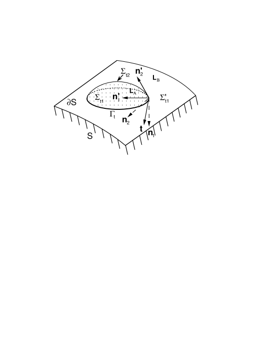
Figure 1: A liquid $L_{A}$ (in drop form) lies on a solid surface $\partial S$. The liquid $L_{A}$ is bordered with a fluid $L_{B}$ and a solid $S$; $\Sigma_{t1}$ is the boundary between liquid $L_{A}$ and solid $S$; $\Sigma^{\prime}_{t1}$ is the boundary between fluid $L_{B}$ and solid $S$, and consequently, $\Sigma_{t1}\cup\Sigma^{\prime}_{t1}=\partial S$; $\Sigma_{t2}$ is the interface between liquid $L_{A}$ and fluid $L_{B}$; $\mathbf{n}_{1}$ and $\mathbf{n}_{2}$ are the unit normal vectors to $\Sigma_{t1}$ and $\Sigma_{t2}$, exterior to the domain of liquid $L_{A}$ and the domain of fluid $L_{B}$, respectively; the edge $\Gamma_{t}$ (or contact line) is common to $\Sigma_{t1}$ and $\Sigma_{t2}$ and $\mathbf{t}$ is the unit tangent vector to $\Gamma_{t}$ relative to $\mathbf{n}_{1}$; $\mathbf{n^{\prime}}_{1}$ and $\mathbf{n^{\prime}}_{2}$ are the binormals to $\Gamma_{t}$ relative to $\Sigma_{t1}$ and $\Sigma_{t2}$, respectively.

Let a liquid $L_{A}$ be in contact with $(i)$ a solid body $S$ on an imprint $\Sigma_{t1}$ of the boundary $\partial S$ of $S$ and $(ii)$ an incompressible fluid $L_{B}$ along an interface $\Sigma_{t2}$ (fig. 1). Let, moreover, the mobile surfaces $\Sigma_{t\alpha}\,(\alpha=1,2)$ be described by the Cartesian equations $f_{\alpha}(t,\mathbf{x})=0\,$ $(\alpha=1,2)$ and let the equations of the common curve $\Gamma_{t}=\Sigma_{t1}\cap\Sigma_{t2}$ be given by

$$f_{1}(t,\mathbf{x})=f_{2}(t,\mathbf{x})=0.$$

For a geometric point M of $\Sigma_{t\alpha}$ with velocity $\mathbf{W}_{\alpha}$ we obtain the kinematic relation

$${\frac{\partial f_{\alpha}}{\partial x^{i}}}W_{\alpha}^{i}+{\frac{\partial f_{\alpha}}{\partial t}}=0,$$

in which the usual convention that over a doubly repeated index summation from $1$ to $3$ is understood. With the notations of fig. 1, if we observe that $\displaystyle n_{\alpha i}=\lambda_{\alpha}(\partial f_{\alpha}/\partial x^{i})$ where $\lambda_{\alpha}$ is a suitable scalar, the celerity of the surface $\Sigma_{t\alpha}$ has the value $\displaystyle c_{\alpha}={\ n_{\alpha i}}W_{\alpha}^{i}=-\lambda_{\alpha}(\partial f_{\alpha}/\partial t)$. This celerity depends only on the coordinates $(t,\mathbf{x})$ of M.

Let the velocity of a point of $\Gamma_{t}$ be denoted by $\mathbf{W}$. We shall denote the unit tangent vector to $\Gamma_{t}$ relative to $\mathbf{n}_{1}$ simply by $\mathbf{t}$ and consequently, $\mathbf{n^{\prime}_{1}}={\mathbf{n}}_{1}\times\mathbf{t}$, $\mathbf{n^{\prime}_{2}}={\mathbf{n}}_{2}\times\mathbf{t}$ (see fig. 1). The velocity of the common line is then expressible as

$$\mathbf{u}=(\mathbf{Id}-\mathbf{t}\otimes\mathbf{t})\mathbf{W}.$$

It is orthogonal to $\Gamma_{t}$ and its expression depends only on the coordinates $(t,\mathbf{x})$ of the point on $\Gamma_{t}$ but it is not necessarily tangential to $\partial S$. Then, $\mathbf{u}=\beta_{1}\mathbf{n}^{\prime}_{1}+\beta_{2}\mathbf{n}^{\prime}_{2}$, where $\beta_{1}$ and $\beta_{2}$ are two scalars. Thus, along $\Gamma_{t}$, $n_{\alpha i}W^{i}=c_{\alpha}$ and $c_{1}=n_{1i}W^{i}=n_{1i}u^{i}=\beta_{2}(\mathbf{n}_{1},\mathbf{n}_{2},\mathbf{t})$, $c_{2}=n_{2i}W^{i}=n_{2i}u^{i}=\beta_{1}(\mathbf{n}_{2},\mathbf{n}_{1},\mathbf{t})$. Consequently,

$$\mathbf{u}={\frac{c_{2}\,\mathbf{n}^{\prime}_{1}-c_{1}\,\mathbf{n}^{\prime}_{2}}{{(\mathbf{n}_{1},\mathbf{t},\mathbf{n}_{2})}}},$$

in which $(\mathbf{a},\mathbf{b},\mathbf{c})$ is the triple product of the three vectors $\mathbf{a},\mathbf{b},\mathbf{c}$. Due to the definitions of $\mathbf{n}_{1}$ and $\mathbf{n}_{2}$, we remark that $(\mathbf{n}_{1},\mathbf{t},\mathbf{n}_{2})>0$.

The kinematics of fluids in the vicinity of the contact line will be axiomatized as follows:

$\Sigma_{t1}$ is a part of the surface of the solid $S$. Liquid $L_{A}$ adheres to $\partial S$ in the sense of the no-slip condition previously proposed. $\Sigma_{t2}$ is a material surface of liquid $L_{A}$.

At the contact line, the velocity $\mathbf{u}$ may have any direction between $\mathbf{n}_{1}$ and $\mathbf{n}_{2}$, depending upon, how the contact line is approached within $L_{A}$. On the solid surface $\Sigma_{t1}$ of $S$ it is, however, tangential to $\Sigma_{t1}$, so that

$$\mathbf{u}={\frac{c_{2}\,\mathbf{n}^{\prime}_{1}}{{(\mathbf{n}_{1},\mathbf{t},\mathbf{n}_{2})}}}\equiv{\frac{(n_{2i}V_{2}^{i})\,\mathbf{n}^{\prime}_{1}}{{\ (\mathbf{n}_{1},\mathbf{t},\mathbf{n}_{2})}}}\equiv-u\,\mathbf{n}^{\prime}_{1}$$

where $u$ denotes the value of the contact line celerity in the direction liquid $L_{A}$ to fluid $L_{B}$ and $\mathbf{V}_{2}$ is the common velocity of the fluids on $\Sigma_{t2}$. The contact line $\Gamma_{t}$ is not a material line of $L_{A}$; its velocity is different from the velocities of the liquid on $S$ and on $\Sigma_{t2}$.

Figure 2: Typical two-dimensional motion of fluids in contact on a solid surface with a stationary contact line. The wedges formed by $\Sigma_{t1}$, $\Sigma_{t2}$ and $\Sigma_{t2}$, $\Sigma^{\prime}_{t1}$ bound the fluids $L_{A}$ and $L_{B}$. The auxiliary surface $\Sigma_{t3}$ separates $L_{B}$ into two domains. A control surface $\Sigma^{\prime}_{t}$ together with $\Sigma_{t1}$ and $\Sigma^{\prime}_{t1}$ constitute the boundary of a compact domain $D_{t}$ of the two fluids. For explanations, see main text.

The motion of the particles of $L_{A}$ on $\partial S$ and $\Sigma_{t2}$ is comparable with that of an adhesive tape stuck on a wall, the other edge of the adhesive tape being mobile (fig. 2): for $u>0$ (or $c_{2}<0$) the particles of $L_{A}$ belonging to $\Sigma_{t2}$ are driven towards $\Gamma_{t}$ and necessarily adhere to $S$ along $\Sigma_{t1}$. For $u<0$ (or $c_{2}>0$) the result is reversed: the particles of $L_{A}$ belonging to $\Sigma_{t1}$ reach $\Gamma_{t}$ and are driven towards $\Sigma_{t2}$.

In fig. 3 the motion of the fluids is sketched. The two manifolds $\Sigma_{t1}$ and $\Sigma_{t2}$ constitute two sheets of the same material surface. The motion of the liquid $L_{A}$ is represented by using a continuous mapping $\varphi$ from a half reference space $D_{0}(L_{A})$ bounded by $\partial S_{0}$, see fig. 3, onto the actual domain $D_{t}(L_{A})$ occupied by $L_{A}$. The domain $D_{t}(L_{A})$ is included in the dihedral angle formed by $\Sigma_{t1}$ and $\Sigma_{t2}$. The contact line $\Gamma_{t}$ is the image of the mobile curve $\Gamma_{0t}$ on $\partial S_{0}$. Outside $\Gamma_{0t}$, the mapping $\varphi$ is $C^{2}$-differentiable.

Figure 3: In the reference configuration, the two sheets of the same material surface of fluid $L_{A}$ are represented by a manifold $\partial S_{0}$ differentiable along $\Gamma_{0t}$. Its image in present configuration, $D_{t}$ is divided into two differentiable manifolds $\Sigma_{t1},\Sigma_{t2}$ forming a dihedral angle. The common edge $\Gamma_{t}$ is the image of a moving curve $\Gamma_{0t}$ in $\partial S_{0}$. The triad $\mathbf{n}_{0},\mathbf{t}_{0},\mathbf{n}^{\prime}_{0},$ in the reference configuration is transformed by the mapping $\varphi$ into the triad $\mathbf{n}_{1},\mathbf{t},\mathbf{n}^{\prime}_{1}$ or the triad $\mathbf{n}_{2},\mathbf{t},\mathbf{n}^{\prime}_{2}$ depending on whether its image is associated with the manifold $\Sigma_{t1}$ or the manifold $\Sigma_{t2}$. For other notations see main text.

A second fluid $L_{B}$ occupies the supplemental dihedral angle $(\Sigma^{\prime}_{t1},\Sigma_{t2})$. The conditions of motion are the opposite to those of $L_{A}$. The material surface $\Sigma_{t2}$ is the common interface between $L_{A}$ and $L_{B}$. Provided the fluids are not inviscid, the velocities of the fluids $L_{A}$ and $L_{B}$ are equal along $\Sigma_{t2}$. Moreover, for liquid $L_{A}$, if $u>0$, the particles of $L_{A}$ are driven towards $\Gamma_{t}$ and adhere to $S$ along $\Sigma_{t1}$. The particles of $L_{B}$ are also driven towards $\Gamma_{t}$; if they adhere to $S$ along $\Sigma^{\prime}_{t1}$, the contact line goes through the two fluids $L_{A}$ and $L_{B}$ along the solid wall $\partial S$, (if $u<0$, a change in the time direction along the trajectories leads to analogous consequences). This is in direct conflict with the fact that $\Gamma_{t}$ belongs to the interface $\Sigma_{t2}$ separating $L_{A}$ and $L_{B}$. To remove this contradiction, it is possible to separate the fluid $L_{B}$ in two parts with a material surface $\Sigma_{t3}$ (see figs. 2 and 3). $\Sigma^{\prime}_{t1}$ and $\Sigma_{t3}$ are the two sheets of the same material surface for a domain $D^{\prime}_{t}(L_{B})$ of the fluid $L_{B}$ within the wedge formed by the dihedral angle ($\Sigma^{\prime}_{t1}$, $\Sigma_{t3}$). The sheets $\Sigma_{t2}$ and $\Sigma_{t3}$ constitute two parts of the same material surface for a domain $D_{t}^{\prime\prime}(L_{B})$ of the fluid $L_{B}$ within the wedge formed by the dihedral angle ($\Sigma_{t2},\Sigma_{t3}$). The two domains $D^{\prime}_{t}(L_{B})$ and $D_{t}^{\prime\prime}(L_{B})$ with common material surface $\Sigma_{t3}$ - across which velocity is continuous - constitute two independent fluid domains which do not mix. For the domain $D_{t}^{\prime}(L_{B})$, the conditions in the vicinity of the contact system are similar to those of liquid $L_{A}$. Velocities which are discontinuous and multi-valued on $\Gamma_{t}$, are compatible with the movements of fluids $L_{A}$ and $L_{B}$ within the domains $D_{t}(L_{A})$, $D_{t}^{\prime}(L_{B})$ and $D_{t}^{\prime\prime}(L_{B})$.

3 Equations of motion and boundary conditions revisited

The fundamental law of dynamics is expressed in the form of the Lagrange-d’Alembert principle of virtual work applied to any compact domain of the two fluids $L_{A}$ and $L_{B}$.

Any compact domain $D_{t}$ made up of the two fluids $L_{A}$ and $L_{B}$ is bounded by $\Sigma_{t}$. The boundary $\Sigma_{t}$ is constituted of $\Sigma_{t1}$, $\Sigma^{\prime}_{t1}$ and a complementary surface $\Sigma^{\prime}_{t}$ which is not in contact with the solid surface $\partial S$: $\Sigma_{t}=\Sigma_{t1}\cup\Sigma^{\prime}_{t1}\cup\Sigma^{\prime}_{t}$ (fig. 2). In a Galilean frame, the virtual work due to the forces applied to $L_{A}$ and $L_{B}$  (including inertial forces but without forces due to capillarity) is in the general form

$$\int_{D_{t}}[\ (\phi_{i}-\rho\ a_{i})\ \zeta^{i}+(p\ \delta_{i}^{j}-Q_{i}^{j})\ \zeta_{,j}^{i}\ ]\,dv+\int_{\Sigma_{t}}P_{i}\ \zeta^{i}\,da.$$

Here, $dv$, $da$ (and later $dl$) are the volume, area (and later line) increments, $\zeta$ denotes any virtual displacement field, $\phi$ the volumetric forces, $\rho$ the density, $\mathbf{a}$ the acceleration vector, $\mathbf{Q}$ the viscous stress tensor and $p$ the pressure. Moreover, the stress vector $\mathbf{P}$ describes the action of the external media on $\Sigma_{t}$. A contribution along $\Gamma_{t}$ is not accounted for.

In continuum mechanics, fluid-fluid and fluid-solid interfaces are differentiable manifolds endowed with surface energies. We denote $\sigma_{AB},\sigma_{AS}$ and $\sigma_{BS}$, the surface energies of interfaces liquid $L_{A}$-fluid $L_{B}$, liquid $L_{A}$-solid $S$ and fluid $L_{B}$-solid $S$, respectively. It is usual to define a measure of energy on interfaces denoted by $\sigma\,da$, where $\sigma$ stands for $\sigma_{AB},\sigma_{AS}$ or $\sigma_{BS}$ following the interfaces between the fluids and the solid. The total energy of capillarity of the interfaces $\Sigma_{t1},\Sigma^{\prime}_{t1}$ and $\Sigma_{t2}$ is

$$E=\int_{\Sigma_{t}}\sigma\ da.$$

For any virtual displacement field, the variation of E is (Gouin and Kosiński, [12]),

$$\delta E=\int_{\Sigma_{t}}\ \Big{[}\ \delta\sigma-\left({\frac{2\sigma}{R_{m}}}\ n_{i}+\left(\delta_{i}^{j}-n^{j}n_{i}\right)\sigma_{,j}\right)\zeta^{i}\ \Big{]}\ da$$

$$+\int_{\Gamma_{t}}\Big{(}(\sigma_{AS}-\sigma_{BS})\,{n^{\prime}}_{1i}+\sigma_{AB}\;{n^{\prime}}_{2i}\Big{)}\ \zeta^{i}\,dl,$$

where the scalar $\delta\sigma$ is the variation of the surface energy $\sigma$ associated with the displacement $\zeta$; vector $\mathbf{n}$ ($n^{i})$ and scalar $R_{m}$ stand for the unit normal vector and the mean radius of curvature to $\Sigma_{t1},\Sigma^{\prime}_{t1}$ or $\Sigma_{t2}$, respectively.
The surface energy $\sigma_{AB}$ between the liquid $L_{A}$ and the fluid $L_{B}$ is positive and constant (Rowlinson and Widom, [27]). Generally, a fluid-solid surface energy depends on the fluid which is in contact with the solid, the geometrical and physico-chemical properties of the solid, the microscopic asperities or the presence of a surfactant. The simplest case occurs when the surface energy is defined as a function of the position on the surface ($\mathbf{x}\in\Sigma_{t}\rightarrow\sigma(\mathbf{x},t)$).

Hereafter considering such a case, the virtual work due to the forces of capillarity applied to $L_{A}$ and $L_{B}$  is simply

$$\int_{\Sigma_{t}}{\frac{{2\sigma}}{R_{m}}}\ n_{i}\ \zeta^{i}\ da-\int_{\Gamma_{t}}\Big{(}(\sigma_{AS}-\sigma_{BS})\,{n^{\prime}}_{1i}+\sigma_{AB}\;{n^{\prime}}_{2i}\Big{)}\ \zeta^{i}\,dl,$$

and relations (1), (2) lead, after execution of the variations and performing integration by parts in several volume and surface terms, to the expression, denoted by $\delta T$, of the virtual work by forces applied to the domain $D_{t}$

$$\delta T=\int_{D_{t}}[\,(\phi_{i}-\rho a_{i}-p_{,i}+Q_{i,j}^{j})\ \zeta^{i}\,]\,dv$$

$$+\int_{\Sigma^{\prime}_{t}}\left(P_{i}+p\,n_{i}-Q_{i}^{j}\ n_{j}\right)\zeta^{i}\ da\,+\int_{\partial S}\left(P_{i}+({\frac{2{\sigma_{S}}}{R_{m}}}+p)\ n_{1i}-Q_{i}^{j}\ n_{1j}\right)\zeta^{i}\ da$$

$$+\int_{\Sigma_{t2}}\left((\ {\frac{2{\sigma_{AB}}}{R_{m}}}+p_{A}-p_{B})\ n_{2i}-(Q_{Ai}^{j}-\ Q_{Bi}^{j})\ n_{2j}\right)\zeta^{i}\,da$$

$$-\int_{\Gamma_{t}}\Big{(}(\sigma_{AS}-\sigma_{BS})\,{n^{\prime}}_{1i}+\sigma_{AB}\;{n^{\prime}}_{2i}\Big{)}\ \zeta^{i}\,dl.$$

Unit normal vectors $\mathbf{n_{1}}$ and $\mathbf{n_{2}}$ are exterior to the domain of liquid $L_{A}$ and fluid $L_{B}$, respectively; $\sigma_{S}$ is called $\sigma_{AS}$ or $\sigma_{BS}$ depending upon which fluid is in contact with $\partial S$, and $Q_{i}^{j}$ is called $Q_{Ai}^{j}$ or $Q_{Bi}^{j}$, respectively depending upon which fluid is in contact with $\Sigma^{\prime}_{t}$ and $\partial S$. We emphasize that it is not necessary for $D_{t}$, $\Sigma^{\prime}_{t}$ and $\Gamma_{t}$ to be material. Finally, virtual displacements are tangential to the solid surface $\partial S$ ($\displaystyle\mathrm{on}\,\,\partial S,\,\,n_{1i}\zeta^{i}=0$).

The expression of the Lagrange-d’Alembert principle is (Germain, [11]):

For any $\zeta$ such that on $\displaystyle\partial S,\,\,n_{1i}\zeta^{i}=0,\ then\ \delta T=0$.

We emphasize that this principle is not associated with a variational approach and there is no variational principle in it: $\delta T$ is not the Frechet derivative of a functional (Gurtin, [13]). Only for equilibrium, and due to the fact that the viscous stress tensor is null, the minimization of energy (this is a variational principle) coincides with this approach. Such a method is relevant to the theory of distributions where $\zeta$ are vector fields of class $C^{\infty}$ with compact support (Schwartz, [31]).

The equations of motion and natural boundary conditions that emerge from it are as follows:

Equations of motion

$$\rho a_{i}+p_{,i}=\phi_{i}+Q^{j}_{i,j}.$$

Conditions on the liquid $L_{A}$ - fluid $L_{B}$ interface $\Sigma_{t2}$

$${\frac{{2\sigma_{AB}}}{R_{m}}}n_{2i}=(Q_{Ai}^{j}-Q_{Bi}^{j})n_{2j}+(p_{B}-p_{A})n_{2i},$$

which is the dynamic form of the Laplace equation.

Conditions on the boundary $\Sigma^{\prime}_{t}$

$$P_{i}=-p\,n_{i}+Q_{i}^{j}\,n_{j},$$

which is the classical expression of the balance of stresses for viscous fluids.

Conditions on the surface $\partial S=\Sigma_{t1}\cup\Sigma^{\prime}_{t1}$

Expression (3) of the virtual work and the Lagrange-d’Alembert principle imply: For any $\zeta$ such that $\displaystyle\mathrm{on}\,\,\partial S,\,n_{1i}\zeta^{i}=0,$

$$\int_{\partial S}\left(P_{i}+({\frac{2{\sigma_{S}}}{R_{m}}}+p)\ n_{1i}-Q_{i}^{j}\ n_{1j}\right)\zeta^{i}\ da=0.$$

Consequently, there exists a scalar field $\chi$ of Lagrange multipliers defined on $\partial S$ such that (Kolmogorov and Fomin, [19])

$$P_{i}\ =Q_{i}^{j}\,n_{1j}-({\frac{{2\sigma_{S}}}{R_{m}}}+p)\ n_{1i}+\chi\ n_{1i}.$$

Generally $\mathbf{P}$ is not collinear to $\mathbf{n}_{1}$ and $\chi$ is an additional unknown scalar.

Conditions on the contact line $\Gamma_{t}$

Due to the condition on $\partial S,\ n_{1i}\zeta^{i}=0$, a virtual displacement is expressed at any point of the contact line $\Gamma_{t}$ in the form

$${\mbox{{\boldmath$\zeta$}}}=\kappa\ \mathbf{t}+\upsilon\ \mathbf{n^{\prime}}_{1},$$

where the two scalar fields $\kappa$ and $\upsilon$ are defined on $\Gamma_{t}$. For any field $\zeta$ in the form (8), the contribution of $\,\int_{\Gamma_{t}}\Big{(}(\sigma_{AS}-\sigma_{BS})\;n_{1i}^{\prime}+\sigma_{AB}\;n_{2i}^{\prime}\Big{)}\,\zeta^{i}\,dl$ in relation (3) yields

$$\int_{\Gamma_{t}}\Big{(}(\sigma_{AS}-\sigma_{BS})\;n_{1i}^{\prime}+\sigma_{AB}\;n_{2i}^{\prime}\Big{)}\,(\kappa\ t^{i}+\upsilon\ {{n^{\prime}}_{1}}^{i})\,dl=0$$

In the general case, since $\mathbf{n^{\prime}}_{1}=\mathbf{n}_{1}\times\mathbf{t}$ and $\mathbf{n^{\prime}}_{2}=\mathbf{n}_{2}\times\mathbf{t}$, expression (9) implies

$$\sigma_{AS}-\sigma_{BS}\ +\sigma_{AB}\,\mathrm{cos}\ \theta_{i}\,=0,$$

where $\theta_{i}$ is the angle between $\mathbf{n^{\prime}}_{1}$ and $\mathbf{n^{\prime}}_{2}$. This angle named intrinsic contact angle in the literature (Wolansky and Marmur, [36]), is the angle in a plane that is normal to $\partial S$ and $\Gamma_{t}$ between tangents in $O$ parallel to $\Sigma_{t2}$ and $\partial S$ (see fig. 4).

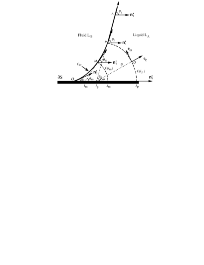
Figure 4: Cross section $C_{t2}$ of the fluid-fluid interface and the solid wall in the plane $(O,\mathbf{n^{\prime}}_{1},\mathbf{n^{\prime}}_{2})$. The contact line is reduced in this figure to the point $O$. The intrinsic angle $\theta_{i}$ is the angle between $\mathbf{n^{\prime}}_{1}$ and $\mathbf{n^{\prime}}_{2}$. At any generic point of $C_{t2}$, the angle between $\mathbf{n^{\prime}}_{1}$ and the tangent to $C_{t2}$ is denoted by $\theta$; thus, at the points $M$, $P$ and $A$, the angle $\theta$ is denoted by $\theta_{m}$, $\theta_{p}$ and $\theta_{a}$, (see main text in section 3). The intersections of the tangent lines to $C_{t2}$ in $M$ and $P$ with the axis $O\,\mathbf{n^{\prime}}_{1}$ are denoted by $I_{m}$ and $I_{p}$. The arcs of circles $C(I_{m})$ and $C(I_{p})$ of centers $I_{m}$ and $I_{p}$ and radius $I_{m}M$ and $I_{p}P$ intersect the axis $O\,\mathbf{n^{\prime}}_{1}$ at points $J_{m}$ and $J_{p}$, respectively. A point $Q$ of $C(I_{p})$ is represented by $(\varrho,\omega)$ in the polar coordinate system of pole $I_{p}$ and polar axis $O\,\mathbf{n^{\prime}}_{1}$ (see main text in subsection 5.2).

At point $O$ of the contact line $\Gamma_{t},$ let us consider the section of the $L_{A}$-$L_{B}$ interface in the plane erected by $\ \mathbf{n^{\prime}}_{1}$ and $\mathbf{n^{\prime}}_{2}$. Let the curvature of the planar section $C_{t2}$ of $\Sigma_{t2}$ be $R^{-1}$. For a two-dimensional flow, the mean curvature of the surface $\Sigma_{t2}$ is $2\,R_{m}^{-1}=R^{-1}$. At a generic point of $C_{t2}$, the angle between $\mathbf{n^{\prime}}_{1}$ and the tangent to $C_{t2}$ is denoted by $\theta$. This angle depends on the choice of the point and on the fluid flow. Since the surface energy $\sigma_{AB}$ between two fluids is constant and $R=dl/d\theta$, we obtain,

$$\int_{O}^{P}\frac{\sigma_{AB}}{R}\mathrm{\ }\sin\theta\ dl\equiv\sigma_{AB}(\cos\theta_{i}-\cos\theta_{p}),$$

where $\theta_{p}$ is the value of $\theta$ at the point $P$. Relation (5) yields

$$\frac{\sigma_{AB}}{R}=(Q_{Ai}^{j}-Q_{Bi}^{j})n_{2}^{i}n_{2j}+p_{B}-p_{A},$$

and, consequently, relations (10), (11) yield

$$\sigma_{AS}-\sigma_{BS}+\sigma_{AB}\,\mathrm{cos}\ \theta_{p}\,+\int_{O}^{P}\left((Q_{Ai}^{j}-Q_{Bi}^{j})\ n_{2}^{i}n_{2j}+p_{B}-p_{A}\right)\mathrm{sin}\ \theta\ dl=0.$$

4 A creeping flow example of non-Newtonian fluids

4.1 The Huh and Scriven model revisited

To understand more precisely the behaviour of a liquid near a moving solid-liquid-fluid contact line, we reconsider the situation of two-dimensional flows proposed by Huh and Scriven, [18]. Let us recall the main results of their article (see fig. 2):

A flat solid surface in translation at a steady velocity $\mathbf{U}$ is inclined from a flat interface between a liquid $L_{A}$ and a fluid $L_{B}$ (here, the angle $\theta$ of fig. 4 is constant, independent of the generic point of $C_{t2}$). The contact line velocity with respect to the solid is $-\mathbf{U}$; thus in the notations of section 2, we obtain $\mathbf{U}=u\,\mathbf{n}_{1}^{\prime}$. In a two-dimensional situation of the plane $(O,\mathbf{n}_{1}^{\prime},\mathbf{n}_{2}^{\prime})$, it is convenient to take the contact line intersection point $O$ as the origin of a polar coordinate system $(r,\varphi)$ and $O\,\mathbf{n}_{1}^{\prime}$ as the reference polar axis. The two bulks are incompressible Newtonian fluids. In term of the stream function $\psi(r,\varphi)$ for two-dimensional steady flows, the velocity is

$$\mathbf{V}=\;v_{r}\mathbf{e}_{r}+v_{\varphi}\mathbf{e}_{\varphi},\,{\mathrm{w}ith}\,\,\,v_{r}=-{1\over r}{\partial\psi\over\partial\varphi},\,v_{\varphi}={\partial\psi\over\partial r},$$

and ($O,\mathbf{e}_{r},\mathbf{e}_{\varphi})$ as the mobile polar frame. In the creeping flow approximation of a viscous fluid, Eq. (4) leads to the linearized Navier-Stokes equation and consequently to the biharmonic equation $\displaystyle\nabla^{4}\psi=0\,$, where $\displaystyle\nabla^{2}$ and $\displaystyle\nabla^{4}$ are respectively the Laplacian and bi-Laplacian operators (Moffat, [23]; Bataille, [1]). A solution is in the form:

$$\psi(r,\varphi)\equiv rf(\varphi)$$

which leads to the ordinary differential equation

$$f(\varphi)+2f^{\prime\prime}(\varphi)+f^{(IV)}(\varphi)=0,$$

and thus to the general solution

$$\psi(r,\varphi)=r(a\ \mathrm{sin}\ \varphi+b\ \mathrm{cos}\ \varphi+c\ \varphi\ \mathrm{sin}\ \varphi+d\ \varphi\ \mathrm{cos}\ \varphi),$$

which holds for either fluid.

The boundary conditions at the solid wall and the liquid-fluid interface are:

$(i)$ a vanishing normal component of the velocity at the solid surface and interface,

$(ii)$ continuity of the velocity at the interface,

$(iii)$ continuity of the tangential stress at the interface,

$(iv)$ non tangential relative motion of the fluids at the solid surface except at the contact line.

These eight linear conditions yield the values of coefficients $a,b,c,d$ for the two fluids $L_{A}$ and $L_{B}$. If the dynamic viscosity coefficients are identical, the eight integration constants are:

$$\left\{\begin{array}[]{l}\displaystyle a_{A}=-u\,\theta D(\theta)[\ \pi-\theta+\mathrm{sin}\ \theta\ \mathrm{cos}\ \theta\ ],\\ \displaystyle a_{B}=u\,D(\theta)[\ (\pi-\theta)(\mathrm{sin}\ \theta\ \mathrm{cos}\ \theta-\theta)+\pi\ \theta\ \mathrm{sin}^{2}\ \theta\ ],\\ \displaystyle b_{A}=0,\\ \displaystyle b_{B}=u\,D(\theta)[\ \pi\ \theta\ \mathrm{sin}\ \theta\ \mathrm{cos}\ \theta-\pi\ \mathrm{sin}^{2}\ \theta\ ],\hskip 128.0374pt(13)_{2}\\ \displaystyle c_{A}=u\,D(\theta)\ (\pi-\theta)\ \mathrm{sin}^{2}\ \theta,\\ \displaystyle c_{B}=-u\,D(\theta)\ \theta\ \mathrm{sin}^{2}\ \theta,\\ \displaystyle d_{A}=u\,D(\theta)[\ (\pi-\theta)\ \mathrm{sin}\ \theta\ \mathrm{cos}\ \theta+\ \mathrm{sin}^{2}\ \theta\ ],\\ \displaystyle d_{B}=u\,D(\theta)[\ -\theta\ \mathrm{sin}\ \theta\ \mathrm{cos}\ \theta+\ \mathrm{sin}^{2}\ \theta\ ]\par\end{array}\right.$$

with $D(\theta)=[\ \theta\ (\pi-\theta)-(\pi-2\theta)\ \mathrm{sin}\ \theta\ \mathrm{cos}\ \theta-\mathrm{sin}^{2}\ \theta\ ]^{-1}$.

No difficulty should arise, in principle, in the determination of $a_{A},\ldots,d_{B}$ for two fluids with distinct dynamic viscosity coefficients. The form of the streamlines as obtained by Huh and Scriven are sketched in fig. 2, and the motion of the contact line fits perfectly with the kinematics as outlined in section 2. Furthermore, if $\mu_{A}=\mu_{B}=\mu$ for all values of the dynamic contact angle $\theta$, the viscous stress components are

$$\tau_{r\varphi}=-\;\frac{\mu}{r}(f+f^{\prime\prime})\ \equiv\ -\ 2\ \frac{\mu}{r}(c\ \mathrm{cos}\ \varphi-d\ \mathrm{sin}\ \varphi),\ \tau_{rr}=\tau_{\varphi\varphi}=0$$

and the pressure field is given by

$$p=p_{0}+\frac{\mu}{r}\;(f^{\prime}+f^{\prime\prime\prime})\equiv p_{0}-2\ \frac{\mu}{r}(c\ \mathrm{sin}\ \varphi\ +d\ \mathrm{cos}\ \varphi),$$

where $p_{0}$ is the hydrostatic pressure (in both formulae phase subscripts have been omitted).

As proved by Huh and Scriven, the dissipation in any domain $D_{t}$ of the fluids containing the contact line $\Gamma_{t}$, $\Big{(}\int_{D_{t}}(\mu/2)\,(f+f^{\prime\prime})^{2}/{r^{2}}\ dv\Big{)},$ and the total traction exerted on the solid surface by the fluid interface are logarithmically infinite. Moreover the normal stress across the fluid interface varies as $r^{-1}$; furthermore, the stress jump should be balanced by the Laplace interfacial tension $\displaystyle\sigma_{AB}\,R^{-1}$ and the curvature $R^{-1}$ does increase indefinitely at the contact line. These are all non-integrable singularities.

4.2 A model of non-Newtonian fluid near the contact line

To avoid the previous paradox of an infinite dissipative function at the contact line, we consider non-Newtonian incompressible fluids with a convenient behaviour of the viscous stress tensor. It is experimentally known that the dynamic viscosity $\mu$ of polymeric liquids depends on the shear rate $\dot{\epsilon}$. The behaviour prevailing in such situations is not well understood. In a wide variety of technological applications, liquids are subjected to large shear strain forces. A molecular dynamic investigation of liquids subjected to large shear strain rates has been performed by Heyes et al, [14]. The shearing action has been found to change the liquid structure and reveals a tendency to reduce the shear viscosity (Ryckaert et al, [28]).
In the literature, some empirical formulas for the viscosity obtained by means of a weighted least-squared adjustment were proposed. For example, $\mu(\dot{\epsilon})\simeq\;\mu(0)\;-\;c$ $\dot{\epsilon}^{2}$ was suggested as possible form for the viscosity as a function of $\dot{\epsilon}$ (Heyes et al [14]). Holian and Evans, [16], proposed a representation in the form

$$\mu(\dot{\epsilon})\simeq\;\mu(0)\;-\;c\sqrt{\dot{\epsilon}}.$$

Data for the viscosity of an atomic fluid generated by nonequilibrium molecular dynamic were performed by Ryckaert et al, [28]. They indicated that for shear rates below $10^{12}s^{-1}$, $\mu(\dot{\epsilon})$ does not differ significantly from $\mu(0)$ but that these previous laws are not extendable when $\dot{\epsilon}$ tends to infinity.

We propose a model where the viscous stress tensor $\mathbf{Q}\;$is a function of the strain rate tensor $\displaystyle{\mbox{{\boldmath$\Delta$}}}\equiv({1/2})\left(\nabla\mathbf{V}+(\nabla\mathbf{V})^{t}\right)$. For moderate values of $\Delta$ the fluid is Newtonian and the function is linear. The function deviates from this classical behaviour for large values of $\Delta$. For an isotropic stress tensor of two-dimensional flow, the Rivlin-Ericksen representation theorem (Truesdell and Noll, [34]) leads to a viscous stress tensor in the form $\mathbf{Q}=\lambda\ \mathbf{I}+2\ \mu{\mbox{{\boldmath$\Delta$}}}$ but $\lambda$ and $\mu$ are non-constant functions of invariants of ${\mbox{{\boldmath$\Delta$}}},$ and $\mu{\mbox{{\boldmath$\Delta$}}}$ is a functional of $\Delta$ where $\mu$ tends to $\mu_{0}\$($\mu_{0}$ being constant) when $\Delta$ tends to zero.
We propose to use a convenient representation of the $\mu$-behaviour in the form

$$\mu=(1-e^{-\gamma})\ \mu_{0}\,\,\,\,\mathrm{with}\,\,\,\,\gamma=\left({\frac{1}{\left\|{\mbox{{\boldmath$\Delta$}}}\right\|\tau_{0}}}\right)^{\xi}$$

where $\left\|{\mbox{{\boldmath$\Delta$}}}\right\|\;=\;\tau^{-1}\;$is the norm of the strain rate tensor, $\tau_{0}$ is a characteristic time of the fluid and $\xi$ is a small parameter ($0<\xi\ll 1$). Then, for very high shear rates $\mu$ behaves as a step function as expected in Ryckaert et al. To fit with relation (14) when $\dot{\epsilon}$ is close to $10^{12}s^{-1},$ we choose $\xi\;=\;0.2\;$ and $\tau_{0}=10^{-14}s$ but many other values can be considered and results of the literature are disparate.
In the following, we take $\xi=0.1\;$and $\tau_{0}=10^{-12}s$ ; then for $\gamma=\gamma_{0}\equiv 4.6$, we obtain $\mu\;=0.99\,\mu_{0}$. We call this $\gamma_{0}$-value the cut-off coefficient. For $\gamma=\gamma_{0},\;\mu\simeq\mu_{0},\;$and the fluid may be considered as Newtonian.

For the Huh and Scriven model of two-dimensional incompressible flows, $\left\|{\mbox{{\boldmath$\Delta$}}}\right\|=\dot{\epsilon}=\displaystyle\left|f+f^{\prime\prime}\right|/(2\ r)$.  When $u=1\ mm.\ s^{-1}$, due to the $\gamma_{0}-$value, considerable variations of $\mu$ occur from the contact line to a distance of $20$ to $30\;$Angströms. The same holds true on the solid wall when $\theta\in\left[5^{{{}^{\circ}}},175^{{{}^{\circ}}}\right]$. Outside these distances from the contact line, the fluids can be considered as Newtonian. Then, $\mu$ tends to zero for very large values of the shear rate, and ${\mathbf{Q}}$ is a function of $\Delta$ which tends to infinity with ${\mbox{{\boldmath$\Delta$}}},$ but weaker than a linear function. The total stress tensor of a fluid is always of the form $-\;p\;$Id $+\;2\;\mu{\mbox{{\boldmath$\Delta$}}}\;$ where $p\;=\Pi-\lambda$ (here $\Pi$ notes the hydrostatic pressure). For steady flows, the equation of motion is

$$\rho\ \mathrm{grad}\ ({\frac{1}{2}}\mathbf{V}^{2})+\rho\ \mathrm{rot}\ \mathbf{V}\times\mathbf{V}+\mathrm{grad}\ p=\mu\,\nabla^{2}\mathbf{V}+2\ {\mbox{{\boldmath$\Delta$}}}{\boldmath.}\mathrm{grad}\ \mu+\rho\ \mathbf{g}$$

where $\mathbf{g}$ denotes the acceleration due to gravity. For a stream function $\psi(r,\varphi)\equiv rf(\varphi)$, we obtain

$$\mu\nabla^{2}\mathbf{V}=-\frac{\mu_{0}\ (1-e^{-\gamma})}{r^{2}}\left((f^{\prime}+f^{\prime\prime\prime})\mathbf{e}_{r}+(f+f^{\prime\prime})\mathbf{e}_{\varphi}\right),$$

$$2\ {\mbox{{\boldmath$\Delta$}}}{\boldmath.}\mathrm{grad}\ \mu=\xi\ \mu_{0}\ \frac{\gamma\ e^{-\gamma}}{r^{2}}\ \left((f^{\prime}+f^{\prime\prime\prime})\mathbf{e}_{r}-(f+f^{\prime\prime})\mathbf{e}_{\varphi}\right),$$

$$\rho\ \mathrm{rot}\ \mathbf{V}\times\mathbf{V\;=}\;-\frac{\rho}{r}\;(f+f^{\prime\prime})\left(f\mathbf{e}_{r}+f^{\prime}\mathbf{e}_{\varphi}\right).$$

The inequalities $0\;<\;\gamma\ e^{-\gamma}\;\leq\;1-e^{-\gamma}$, $\;0<\;\xi\ll\;1$  and the fact that near the contact line $\ 1\ll\;\displaystyle\frac{\mu}{r\rho\ (f+f^{\prime\prime})}\$ yields the approximate form of Eq. (16)

$$\rho\ \mathrm{grad}\ ({\frac{1}{2}}\mathbf{V}^{2})+\mathrm{grad}\ p=\mu\nabla^{2}\mathbf{V}+\rho\ \mathbf{g},$$

which implies

$$\mu\mathrm{\ rot(}\nabla^{2}\mathbf{V)}+\mathrm{grad\;\mu\;\times\;}\nabla^{2}\mathbf{V\;=0}$$

with

$$\mu\ \mathrm{\ rot(}\nabla^{2}\mathbf{V)\;=-\;}\frac{\mu_{0}}{r^{3}}\ (1-e^{-\gamma})\ (f+2f^{\prime\prime}+f^{(IV)})\;\mathbf{k}$$

and

$$\mathrm{grad\;\mu\;\times\;}\nabla^{2}\mathbf{V\;=\;}\xi\ \mu_{0}\ \frac{\gamma\ e^{-\gamma}}{r^{3}}\left(f+f^{\prime\prime}+{\frac{(f^{\prime}+f^{\prime\prime\prime})^{2}}{f+f^{\prime\prime}}}\right)\mathbf{k}$$

where $\mathbf{k}$ denotes the normal vector to the plane of the flows.

From $\ \xi\ \gamma\ e^{-\gamma}\ll\;1-e^{-\gamma},$ we deduce again the Huh and Scriven approximation for the stream function in the form $\psi(r,\varphi)=rf(\varphi)$, with $f(\varphi)+2f^{\prime\prime}(\varphi)+f^{(IV)}(\varphi)=0$.

On the solid wall, adherence conditions are required. This assumption is in agreement with molecular dynamics of fluid flows at solid surfaces:  The non-slip boundary condition appears to be a natural property of a dense liquid interacting with a solid wall with molecular structure and long range force interactions (Koplick, Banavar and Willemsen, [20]). For the non-Newtonian model and for the creeping flow approximation, the general solution $(13)_{1}$ holds true for either fluid. Furthermore, the boundary conditions at the solid wall and at the liquid-fluid interface are the condition $(i)-(iv)$ of subsection 4.1. Consequently, for the non-Newtonian model and for the creeping flow approximation the trajectories and the velocities near the contact line are identical to those of fluids with constant viscosity $\mu_{0}$ in the Huh and Scriven model.

The dissipation $\Xi$ in the domain $V_{l}=\{r\in[0,l],\ \varphi\in[0,\theta],\ z\in[0,L]\}$ (where $z$ denotes the contact line coordinate) is

$$\Xi\ =\int_{V_{l}}tr(\mu{\mbox{{\boldmath$\Delta$}}}^{2})dv=L\ {\frac{\mu_{0}}{2}}\int_{0}^{\theta}\int_{0}^{l}{\frac{{\ 1-e^{-\gamma}}}{r}}\ (f+f^{\prime\prime})^{2}\ dr\ d\varphi.$$

From the inequality $\ 0<1-e^{-\gamma}\leq\gamma$, we deduce

$$\Xi\ \leq\ {\frac{L\ \mu_{0}}{2^{1-\xi}}}\int_{0}^{\theta}\int_{0}^{l}{\ \ \frac{r^{\xi-1}}{\tau_{0}^{\xi}}}\ |f+f^{\prime\prime}|^{2-\xi}\ drd\varphi={\frac{{\ \ L\ \mu_{0\;}l^{\xi}}}{{\xi\ 2^{1-\xi}\ \tau_{0}^{\xi}}}}\int_{0}^{\theta}|f+f^{\prime\prime}|^{2-\xi}\ d\varphi,$$

which proves that the dissipation is finite at the contact line, since $f$ given by $(13)_{1},(13)_{2}$ is bounded.

Other calculations yield a bounded total force exerted on the solid surface by the fluid-fluid interface near the contact line, but another problem associated with the fluid-fluid interface curvature still remains unresolved.

5 Study of a curved interface in the vicinity of the contact line

For a Newtonian fluid in two dimensional flows, the fluid interface curvature should increase rapidly as the contact line is approached. This result is in direct conflict with the hypothesis of section 4 that the fluid interface is perfectly flat. Indeed, Huh and Scriven, [18], pointed out when water at moderate dynamic contact angle wets a surface at $6$ mm.min^-1, the local radius of curvature would have to be about $10^{5}$ time greater than the distance to the contact line and the curvature would be imperceptible by optical means. Nevertheless in such a case, the intrinsic angle $\theta_{i}$ at the contact line may strongly deviate from the angle $\theta_{p}$, (see fig. 4), which is observed at a point $P$ near, but not at, the contact line.

Let us consider results presented in subsection 4.2; the equation of motion (4), boundary condition (5), and calculations of subsection 4.2 yield the pressure field values for the fluids $L_{A}$ and $L_{B}$,

$$p_{B}-p_{A}\;=\;\frac{\mu}{r}\left((f_{B}^{\prime}+f_{B}^{\prime\prime\prime})-(f_{A}^{\prime}+f_{A}^{\prime\prime\prime})\right)\equiv\frac{\,\mu\,u}{r}\ 2\pi\,\mathrm{sin}\ \theta\ D(\theta).$$

As done by Huh and Scriven, we notice that

$$p_{B}-p_{A}\ =\;\frac{\sigma_{AB}}{R},$$

and consequently,

$$\frac{r}{R}=\frac{\mu\;u}{\sigma_{AB}}\ 2\pi\,\mathrm{sin\;}\theta\ D(\theta).$$

For partial wetting, it is easy to compute the value of $2\pi\ \mathrm{sin\,}\theta\ D(\theta)$ numerically; we obtain

$$\frac{\pi}{6}<\theta<\frac{5\;\pi}{6}\ \ \Rightarrow\ \ 4<2\pi\,\mathrm{sin\,}\theta\ D(\theta)<15.$$

When the capillary number $C_{a}=\mu_{0}\,|u|/\sigma_{AB}\$is sufficiently small, (in experiments, $C_{a}$ is often smaller than $10^{-3}$), we deduce $\displaystyle|r/R|\ll 1$; it is all the more true, for a non-Newtonian fluid given by the representation (15), where $\mu$ tends to zero at the contact line.

5.1 Two-dimensional steady flows near the contact line

The conditions and the notations are given in subsection 4.2, but the fluid-fluid interface is curved. The cross section of the fluid-fluid interface and the solid wall is presented on fig. 4. We consider the domain occupied by the two fluids in the immediate vicinity of the contact line and we assume that, along $C_{t2}$

$$\lim_{r\rightarrow\,0\,\,}\frac{r}{R}\equiv\lim_{r\rightarrow\,0\,\,}\frac{r\,d\theta}{dl}=0.$$

Thus, in the immediate vicinity of the contact line, we obtain $|r/R|\ll 1$.
On fig. 4, at the generic point $P$ of $C_{t2}$, the intersection of the tangent line with the axis $0\,{\mathbf{n}}^{\prime}_{1}$ is denoted by $I_{p}$. To each point $I_{p}$ corresponds, in the fluid domains, the arc of a circle, denoted by $C(I_{p})$, with center $I_{p}$ and radius $I_{p}P$. To a point $Q$ of $C(I_{p})$ corresponds the polar coordinates, $(\varrho,\omega)$, associated with the pole $I_{p}$ and the mobile frame $({\mathbf{e}}_{\varrho},{\mathbf{e}}_{\omega})$. The polar coordinates of $P$ are $(\varrho,\theta_{p})$ and will be denoted simply by $(\varrho,\theta)$. Let us denote by $y\equiv\varrho\,{\mathrm{s}in}\,\theta$, the distance from the point $P$ to the solid wall. We deduce, $dy=d\varrho\,{\mathrm{s}in}\,\theta+\varrho\,{\mathrm{c}os}\,\theta\,d\theta$ and due to the differential relation, $dy=dl\,{\mathrm{s}in}\,\theta$, we obtain, $d\varrho/dl=1-\varrho\ {\mathrm{c}otg}\,\theta\ d\theta/dl$. When $\theta\neq 0\ {\mathrm{o}r}\ \pi,\ \lim_{r\rightarrow\,0\,\,}\varrho\ {\mathrm{c}otg}\,\theta\,d\theta/dl=0$ and consequently, when $r\rightarrow 0$, $d\varrho\sim dl$. Let $M$ be another point of $C_{t2}$; we denote $J_{p}$ and $J_{m}$ the intersections of $C(I_{p})$ and $C(I_{m})$ with the axis $O\,{\mathbf{n}}^{\prime}_{1}$; when $M\rightarrow P$, $\|{\mathbf{J}}_{m}{\mathbf{J}}_{p}\|\sim d\varrho$, $\|{\mathbf{I}}_{m}{\mathbf{I}}_{p}\|\sim\varrho\ d\theta/{\mathrm{s}in}\,\theta$ and relation (20) implies, $\lim_{r\rightarrow\,0}(\|{\mathbf{I}}_{m}{\mathbf{I}}_{p}\|/\|{\mathbf{J}}_{m}{\mathbf{J}}_{p}\|)=0$. Thus, in the immediate vicinity of the point $O$, $\|{\mathbf{I}}_{m}{\mathbf{I}}_{p}\|\ll\|{\mathbf{J}}_{m}{\mathbf{J}}_{p}\|$ and the two arcs of circles $C(I_{m})$ and $C(I_{p})$ are distinct. In the following, we prove that, near the point $O$, a point $Q$ of the fluid domains is represented by the orthogonal coordinate system $(\varrho,\omega)$. The equation of the curve $C_{t2}$ can be written in the form $\theta=\vartheta(\varrho)$.

As in section 4 for two-dimensional steady flow, the stream function $\Psi(\varrho,\omega)$ verifies $\nabla^{4}\Psi=0$. We look for a stream function in the form

$$\Psi(\varrho,\omega)\equiv\varrho\ h(\omega,\theta),$$

where $\theta=\vartheta(\varrho)$, and such that the partial derivatives of $h$ with respect to $\omega$ and $\theta$ are bounded. But,

$$d{\mathbf{OQ}}=d{\mathbf{OI}_{p}}+d{{\mathbf{I}}_{p}{\mathbf{Q}}}=\left(\,\frac{\varrho\ d\theta}{{\mathrm{s}in}\,\theta\ d\varrho}\ {\mathbf{n}}^{\prime}_{1}+{\mathbf{e}}_{\varrho}\right)d\varrho+\varrho\ d\omega\ {\mathbf{e}}_{\omega}.$$

Since $\lim_{\varrho\rightarrow\,0}\ \varrho\ d\theta/d\varrho=0$ and $\sin\ \theta\neq 0$, we obtain

$$d{\mathbf{OQ}}=d\varrho\ ({\mathbf{e}}_{\varrho}+{\mathbf{o}}_{1}(\varrho))+\varrho\ d\omega\ {\mathbf{e}}_{\omega},\ \ {\mathrm{w}ith}\ \ \lim_{\varrho\rightarrow\,0}\ {\mathbf{o}}_{1}(\varrho)={\mathbf{0}},$$

and near the point $O$

$$d{\mathbf{OQ}}=d\varrho\ {\mathbf{e}}_{\varrho}+\varrho\ d\omega\ {\mathbf{e}}_{\omega}.$$

Moreover,

$${\mathrm{g}rad}\ \Psi=(h+\varrho\ \frac{\partial h}{\partial\theta}\ \frac{d\theta}{d\varrho})\ {\mathbf{e}}_{\varrho}+\frac{\partial h}{\partial\omega}\ {\mathbf{e}}_{\omega}.$$

and

$${\mathrm{g}rad}\ \Psi=(h+o_{2}(\varrho))\ {\mathbf{e}}_{\varrho}+\frac{\partial h}{\partial\omega}\ {\mathbf{e}}_{\omega},\ \ {\mathrm{w}ith}\ \ \lim_{\varrho\rightarrow\,0}\ o_{2}(\varrho)=0.$$

The velocity is

$${\mathbf{V}}=v_{\varrho}\ {\mathbf{e}}_{\varrho}+v_{\omega}\ {\mathbf{e}}_{\omega}+\,{\mathbf{o}}_{3}(\varrho)\ \ {\mathrm{w}ith},\ \ v_{\varrho}=-\frac{\partial h}{\partial\omega},\ v_{\omega}=h\ \ {\mathrm{a}nd},\ \ \lim_{\varrho\rightarrow\,0}\ {\mathbf{o}}_{3}(\varrho)={\mathbf{0}},$$

and near the contact line

$${\mathbf{V}}=v_{\varrho}\ {\mathbf{e}}_{\varrho}+v_{\omega}\ {\mathbf{e}}_{\omega}.$$

In the following, $o_{n}(\varrho)$ with $n\in N$, denotes a smooth function of the order of $\varrho$ such that $\lim_{\varrho\rightarrow\,0}\ o_{n}(\varrho)=0$. Similarly,

$$\nabla^{2}\Psi={\mathrm{d}iv\ grad(\Psi)}=\frac{1}{\varrho}\ h+\frac{\partial h}{\partial\theta}\ \frac{d\theta}{d\varrho}+\frac{1}{\varrho}\ \frac{\partial^{2}h}{\partial\omega^{2}}+\frac{1}{\varrho}\ o_{{}_{4}}(\varrho)=\frac{1}{\varrho}\ h+\frac{1}{\varrho}\ \frac{\partial^{2}h}{\partial\omega^{2}}+\frac{1}{\varrho}\ o_{{}_{5}}(\varrho),$$

$\displaystyle{\mathrm{g}rad}(\nabla^{2}\Psi)=\left(-\frac{1}{\varrho^{2}}\ (h+\frac{\partial^{2}h}{\partial\omega^{2}})+\frac{1}{\varrho}\ (\frac{\partial h}{\partial\theta}+\frac{\partial^{3}h}{\partial\omega^{2}\partial\theta})\frac{d\theta}{d\varrho}+\frac{1}{\varrho^{2}}\ o_{{}_{6}}(\varrho)\right)\ {\mathbf{e}}_{\varrho}\ \\ +\frac{1}{\varrho^{2}}\ (\frac{\partial h}{\partial\omega}+\frac{\partial^{3}h}{\partial\omega^{3}})\ {\mathbf{e}}_{\omega}=\left(-\frac{1}{\varrho^{2}}\ (h+\frac{\partial^{2}h}{\partial\omega^{2}})+\frac{1}{\varrho^{2}}\ o_{{}_{7}}(\varrho)\right){\mathbf{e}}_{\varrho}+\frac{1}{\varrho^{2}}\ (\frac{\partial h}{\partial\omega}+\frac{\partial^{3}h}{\partial\omega^{3}})\ {\mathbf{e}}_{\omega},$

and finally,

$$\nabla^{4}\Psi=\frac{1}{\varrho^{3}}\ (h+\frac{\partial^{2}h}{\partial\omega^{2}})-\frac{1}{\varrho^{2}}\ (\frac{\partial h}{\partial\theta}+\frac{\partial^{3}h}{\partial\omega^{2}\partial\theta})\frac{d\theta}{d\varrho}+\frac{1}{\varrho^{3}}\ (\frac{\partial^{2}h}{\partial\omega^{2}}+\frac{\partial^{4}h}{\partial\omega^{4}})+\frac{1}{\varrho^{3}}\ o_{{}_{8}}(\varrho)$$

$\displaystyle=\frac{1}{\varrho^{3}}\ (h+2\frac{\partial^{2}h}{\partial\omega^{2}}+\frac{\partial^{4}h}{\partial\omega^{4}})+\frac{1}{\varrho^{3}}\ o_{{}_{9}}(\varrho),$

The principal part of the Laurent expansion in $\varrho\,$ of $\,\nabla^{4}\Psi$ leads to the partial derivative equation

$$h+2\ \frac{\partial^{2}h}{\partial\omega^{2}}+\frac{\partial^{4}h}{\partial\omega^{4}}=0,$$

and the general solution for the principal part of $\Psi$ is

$$\Psi(\varrho,\omega)=\varrho\ (a\ \mathrm{sin}\ \omega+b\ \mathrm{cos}\ \omega+c\ \omega\ \mathrm{sin}\ \omega+d\ \omega\ \mathrm{cos}\ \omega),$$

where $a,b,c,d$ are functions of $\theta$. When $\mu_{A}=\mu_{B}$, the boundary conditions at the solid wall and the conditions $(i)$-$(iv)$ presented in section 4 yield the values of coefficients $a,b,c,d$ for the two fluids $L_{A}$ and $L_{B}$. These values are given by relations $(13)_{2}$, but here, $\theta$ is not constant. The viscous stress components are

$$\tau_{\varrho\omega}=-\;\frac{\mu}{\varrho}(h+\frac{\partial^{2}h}{\partial\omega^{2}})\ \equiv\ -\ 2\ \frac{\mu}{\varrho}\ (c\ \mathrm{cos}\ \omega-d\ \mathrm{sin}\ \omega),\ \tau_{\varrho\varrho}=\tau_{\omega\omega}=0.$$

As in section 4, the pressure field is given by

$$p=p_{0}-2\ \frac{\mu}{\varrho}(c\ \mathrm{sin}\ \omega\ +d\ \mathrm{cos}\ \omega).$$

In partial wetting, the stream function (21) together with relations $(13)_{2}$ show that the partial derivatives of $h$ with respect to $\omega$ and $\theta$ are bounded along $C_{t2}$. Along $C_{t2}$, $p_{A}-p_{B}=\sigma_{AB}/R$ and consequently,

$$\frac{\varrho\,d\theta}{dl}=\frac{\mu u}{\sigma_{AB}}\;2\pi\;\mathrm{sin}\theta\;D(\theta).$$

Furthermore, $\|{\mathbf{\Delta}}\|=\{1/(2\varrho))\}\;|\ h+\partial^{2}h/\partial\omega^{2}|_{\omega=\theta}$. Thus,

$$\|{\mathbf{\Delta}}\|=\frac{|u|}{\varrho}\,|c_{A}\cos\,\theta-d_{A}\sin\,\theta|\equiv\frac{|u|}{\varrho}\,|c_{B}\cos\,\theta-d_{B}\sin\,\theta|\equiv\frac{|u|}{\varrho}\,\sin^{3}\theta\,D(\theta).$$

Let us note that, in the frame $(O,{\mathbf{n}}^{\prime}_{1},{\mathbf{n}}_{1})$, relations $x=\varrho\ {\mathrm{c}os}\,\theta$, $y=\varrho\ {\mathrm{s}in}\,\theta$, $dy=dl\ {\mathrm{s}in}\,\theta$, $\theta_{i}={\mathrm{Arccos}}\{(\sigma_{BS}-\sigma_{AS})/\sigma_{AB}\}$ together with Eq. (22) and relation (15), allow us to obtain the parametric representation of $C_{t2}$ near the solid wall.

Eq. (22) allows us to verify that $\lim_{r\rightarrow\,0\,\,}r\,d\theta/dl=0$ and thus, the choice of the stream function $\Psi$ in the form (21) together with relations $(13)_{2}$ is justified in the vicinity of the point $O$. Let us note that when $u>0$ (resp. $u<0$), $\theta$ is an increasing (resp. decreasing) function of the distance $y$ of a point of $C_{t2}$ to the solid wall. We do notice also that, whereas the curvature of $C_{t2}$ tends to infinity when the point $O$ is approached, the stream function $\Psi$ has the same form as the stream function $\psi$ proposed in subsection 4.2 for a plane interface (a good example of such a curve is given, near $x=0$, by $y=\left|x\right|^{\frac{3}{2}}$ (Voinov, [35])).

5.2 Apparent dynamic contact angle and line friction

Let $A$ be the point of $C_{t2}$ associated with the cut-off coefficient value $\gamma_{0}$, defined in subsection 4.2: the point $A$ is at the border between the Newtonian and the non-Newtonian domains of the fluid flows. We call apparent dynamic contact angle $\theta_{a}$, the value of $\theta$ associated with the point $A$ (see fig. 4). Along the fluid-fluid interface, condition $(Q_{Ai}^{j}-Q_{Bi}^{j})\ n_{2}^{i}n_{2j}=0$, together with relation (12) and $p_{B}-p_{A}=(1/\varrho)\;\mu u\;2\pi\;\mathrm{sin}\theta\;D(\theta)$, imply

$$\sigma_{AS}-\sigma_{BS}+\sigma_{AB}\;\mathrm{\cos\;}\theta_{a}+\nu\;u\;=0,$$

with

$$\nu=\int_{0}^{A}\frac{\mu}{\varrho}\;2\pi\;\mathrm{sin}^{2}\theta\;D(\theta)dl.$$

Relation (23) is a form of Young-Dupré dynamic relation for the apparent dynamic contact angle. We call $\nu$, the line friction. It is easy to verify that the scalar $\nu$ is positive and of the same physical dimension as a dynamic viscosity. This result corresponds to the assumption in the article of Stokes et al, [33], in which they say that there is an additional viscous force on a moving contact line. Other expressions for the line friction have also been proposed (an attempt is done by a thermodynamic point of view in Fan, Gao and Huang, [8]).

In the case of equilibrium, relation (23) yields the static Young-Dupré relation (Levitch, [22])

$$\sigma_{AS}-\sigma_{BS}+\sigma_{AB}\;\mathrm{\cos\;}\theta_{e}=0,$$

in which $\theta_{e}$ is the balance Young angle and $\theta_{e}=\theta_{i}=\theta_{a}$. For any value of the contact line celerity, relations (23) and (24) yield, implicitly, the apparent dynamic contact angle $\theta_{a}$. With the formula (23), a simple explanation of a well-known experimental result (Dussan, [6]), may also be corroborated: with the advance of the contact line, $u$ is positive and the apparent dynamic contact angle $\theta_{a}$ is larger than the equilibrium angle $\theta_{e}$. This result is reversed when $u$ is negative.

5.3 Numerical investigations of the apparent dynamic contact angle and the line friction

Hoffman, [17], Legait and Sourieau, [21], Ramé and Garoff, [26], and many other authors experimentally observe that, near the contact line, for slow motions, the apparent dynamic contact angle seems independent of the microscopic distance to the solid surface. Let us verify numerically this observation.

Using the relations $y=\varrho\;\mathrm{sin}\;\theta$ and $dy=dl\;\mathrm{sin}\;\theta$, relation (22) implies

$$\frac{dy}{y}=\frac{\sigma_{AB}}{\mu\;u\;2\pi\;\mathrm{sin}\;\theta\;D(\theta)}\ d\theta.$$

Let us consider a point $N$ of $C_{t2}$ in the Newtonian domain of the fluid flows. Then,

$$\ln(\frac{y_{n}}{y_{a}})=\int_{\theta_{a}}^{\theta_{n}}\frac{\sigma_{AB}}{\mu_{0}\;u\;2\pi\;\mathrm{sin}\;\theta\;D(\theta)}\ d\theta,$$

where $y_{a}$ and $y_{n}$ denote the distances of points $A$ and $N$ to the solid wall. In partial wetting, when $\pi/6<\theta<5\pi/6$, then $0<2\pi\;\mathrm{sin}\;\theta\;D(\theta)<15$ and if $u>0$,

$$0<\theta_{n}-\theta_{a}<15\ C_{a}\ \ln(\frac{y_{n}}{y_{a}}).$$

If we consider the case when $y_{n}=10^{4}\ y_{a}$, a crude approximation yields $\theta_{n}-\theta_{a}<140\ C_{a}$ and thus $\theta_{n}-\theta_{a}$ tends to zero with $C_{a}$. For example, when $C_{a}=10^{-4}$, we obtain $\theta_{n}-\theta_{a}<0.014$ radian, (i.e. $0.8$ degree), and the apparent dynamic contact angle seems independent of the distance of the point $N$ to the solid wall: in the lubrication approximation for two dimensional flows, Eq. (23) expresses the behaviour of the apparent dynamic contact angle independently of any microscopic distance to the contact line. This result is in accordance with Seppecher’s calculations [29].

Let us estimate an order of magnitude of the line friction. Along $C_{t2}$, Eq. (21) implies that, for each fluid, $|\,h+\partial^{2}h/\partial\omega^{2}|_{{}_{\omega=\theta}}=|u|\,2\,\mathrm{sin}^{3}\theta\,D(\theta)$. When $\xi=0.1$, a numerical computation yields

$$\frac{\pi}{6}<\theta<\frac{5\;\pi}{6}\ \ \Rightarrow\ \ 1.015\ |u|^{\xi}<|\ h+\frac{\partial^{2}h}{\partial\omega^{2}}\ |_{{}_{\omega=\theta}}^{\xi}<1.032\ |u|^{\xi}.$$

Taking into account the norm $\|\mathbf{\Delta}\|$ of the strain rate tensor along $C_{t2}$, relation (15) yields a value of $\gamma$ such that

$$\gamma\simeq\frac{1}{1.02}\Big{(}\frac{2\ \varrho}{\tau_{0}u}\Big{)}^{\xi},$$

and $d\gamma/\gamma=\xi\ d\varrho/\varrho$. Then, relation (24) allows us to obtain the value of the line friction

$$\nu=\frac{2\pi\mu_{0}}{\xi}\,\int_{0}^{\gamma_{0}}\mathrm{sin}^{2}\theta\;D(\theta)\ \frac{1-e^{-\gamma}}{\gamma}\ d\gamma.$$

Since $\mathrm{sin}^{2}\theta\,D(\theta)>0$, we obtain

$$\nu=\frac{2\pi\mu_{0}}{\xi}\ \mathrm{sin}^{2}\theta_{r}\;D(\theta_{r})\int_{0}^{\gamma_{0}}\frac{1-e^{-\gamma}}{\gamma}d\gamma,\ \ {\mathrm{w}ith}\ \ \theta_{r}\in[\;\theta_{i},\theta_{a}\;]$$

in which $\theta_{r}$ is a convenient angle. Due to $\displaystyle\int_{0}^{\gamma_{0}}(1/\gamma)(1-e^{-\gamma})d\gamma\simeq 1,$ we obtain

$$\nu=\frac{2\pi\mu_{0}}{\xi}\ \mathrm{sin}^{2}\theta_{r}\;D(\theta_{r}).$$

In partial wetting, a numerical computation implies

$$\frac{\pi}{6}<\theta_{r}<\frac{5\;\pi}{6}\ \ \Rightarrow\ \ 0.68<\mathrm{sin}^{2}\theta_{r}\;D(\theta_{r})<1.17,$$

and consequently

$$42\ \mu_{0}<\nu<73\ \mu_{0}.$$

Eq. (10) and Eq. (23) imply $|\cos\,\theta_{a}-\cos\,\theta_{i}|<\nu\,|u|/\sigma_{AB}$. Taking into account inequalities (26), we obtain $|\cos\,\theta_{a}-\cos\,\theta_{i}|<73\,C_{a}$. In the partial wetting case, for $\theta\in(\pi/6,5\,\pi/6)$, then $|\,\sin\big{(}\,(\theta_{a}-\theta_{i})/2\,\big{)}\,|<73\,C_{a}$ and the derivative of $\sin^{2}\theta\;D(\theta)$ belongs to $(-1,1)$; we can deduce $|\sin^{2}\,\theta_{r}\,D(\theta_{r})-\sin^{2}\theta_{a}\,D(\theta_{a})|<2\,{\mathrm{A}rcsin}(73\,C_{a})$. This crude approximation proves that for $C_{a}$ sufficiently small, $\sin^{2}\theta_{r}\;D(\theta_{r})$ is close to $\sin^{2}\theta_{a}\;D(\theta_{a})$ (for example, when $C_{a}=10^{-4}$, we obtain $|\sin^{2}\,\theta_{r}\,D(\theta_{r})-\sin^{2}\theta_{a}\,D(\theta_{a})|<0.015$). Replacing $D(\theta_{a})$ by its explicit expression sets the approximative relation of the line friction :

$$\nu=\frac{2\pi\mu_{0}}{\xi}\ \Big{(}\;\frac{\mathrm{sin}^{2}\,\theta_{a}}{\theta_{a}\ (\pi-\theta_{a})-(\pi-2\;\theta_{a})\ \mathrm{sin}\ \theta_{a}\ \mathrm{cos}\ \theta_{a}-\mathrm{sin}^{2}\ \theta_{a}}\;\Big{)}.$$

6 Concluding remarks

In this paper, the dynamical problem of the contact of two non-Newtonian viscous fluids $L_{A}$ and $L_{B}$ with a solid was analyzed. Except at the contact line, these fluids were assumed to adhere to the solid and to each other. Then, the principle of virtual work allows us to obtain the governing equations and boundary conditions. It was shown that the equations of motions and boundary conditions lead to streamlines near the contact line similar to those of a Newtonian fluid endowed with a dynamic viscosity which is, when the strain rate tensor tends to zero, the limit of the dynamic viscosity of the non-Newtonian fluid. The analyze of the stress tensor and the dissipative function near the contact line leads to several remarks and conclusions:

For dissipative movements, a viscous stress tensor $Q_{i}^{j}$ was added to the pressure term and in the expression of virtual work, the dissipative terms were distributed within the volume as $Q_{i,j}^{j}$ and on the surfaces as $-Q_{i}^{j}n_{\alpha j}$. In magnitude, the surface tension is comparable with the bulk stress despite the fact that the thickness of the interfacial layer, where the surface tension acts, is negligible compared to the characteristic length scale in the bulk: although the interfacial layer is very thin, the intermolecular forces which act on it and give rise to the surface tension are very strong so that the result is finite. Huge variations of the fluid velocity appear at the three-phase contact line. The only physical factor, which achieves to magnify its role, does not come from intermolecular forces but from the discontinuity of the velocity at the contact line and consequently from the viscosity along the contact line when the thickness of the contact line region tends to zero. In the immediate vicinity of the contact line, the viscous stresses yield a friction force which acts on the fluid-fluid interface and is balanced by strong capillary tensions associated with the curvature of the fluid-fluid interface. Consequently, expression (23) introduces a new term associated with the contact line $\Gamma_{t}$.

Creeping flow of a Newtonian fluid is unrealistic at the corner of a moving contact line. Nevertheless, the system that is based on Eq. (4), boundary conditions (5), (6), adherence assumption on solid surfaces together with the dynamic Young-Dupré relation (23) for the apparent contact angle which accommodates the behaviour of the non-Newtonian fluid domain in the immediate vicinity of the contact line poses a problem of slow fluid motion. This result, in agreement with experiments and molecular investigations, is brought out by means of the analytic representation of the streamlines on Newtonian behaviour; however, other non-Newtonian fluid behaviour is used to arrive at bounded dissipative functions near the contact line.

For slow movements we are able to give a model which provides answers to the previous questions:

- The contact line is a non material line and acts in a similar way as a shock line.

- The velocity fields are multivalued on the line.

- The paradox of infinite viscous dissipation is removed.

- Adherence and boundary conditions on surfaces and interfaces are preserved, but a dynamic Young-Dupré relation derived by the virtual work principle yields the apparent dynamic contact angle as an implicit function of the contact line celerity. The apparent dynamic contact angle is the only pertinent Young angle from a continuum mechanics point of view.

- For partial wetting, and for a sufficiently small capillary number, the concept of line friction is associated with the apparent contact angle.

The contact angle hysteresis phenomenon and the modelling of experimentally well-known results that express the dependence of the dynamic contact angle on the celerity of the line are important phenomena. In part 2, Eq. (23) allows us to obtain an explanation of the contact-angle hysteresis in the advance and retreat of slowly moving fluids on a solid surface.

References

- [1] Bataille J (1966) Etude de l’écoulement au voisinage du ménisque séparant deux fluides se déplaçant lentement entre deux plaques planes parallèles ou dans un tube capillaire. C.R. Acad. Sci. Paris A262: 843-846
- [2] Bazhelakov IB, Chesters AK (1996) Numerical investigation of the dynamic influence of the contact line region on the macroscopic meniscus shape. J. Fluid Mech. 329: 137-146
- [3] Blake TD, Bracke M, Shikhmurzaev YD (1999) Experimental evidence of nonlocal hydrodynamic influence on the dynamic contact angle. Physics of Fluids 11: 1995-2007
- [4] Cox RG (1986) The dynamics of the spreading of liquids on a solid surface. Part 1 Viscous flow, Part 2 Surfactants. J. Fluid Mech. 168: 169-220
- [5] Dussan V EB, Davis SH (1974) On the motion of a fluid-fluid interface along a solid surface. J. Fluid Mech. 65: 71-95
- [6] Dussan V EB (1979) On the spreading of liquids on solid surfaces: static and dynamic contact-lines. Annual Rev. Fluid Mech. 11: 371-400
- [7] Dussan V EB, Ramé E, Garoff S (1991) On identifying the appropriate boundary conditions at a moving contact-line: an experimental investigation. J. Fluid Mech. 230: 97-116
- [8] Fan H, Gao YX, Huang XY (2001) Thermodynamics modeling for moving contact line in gas/liquid/solid system: capillary rise problem revisited. Physics of Fluids 13: 1615-1623
- [9] de Gennes PG (1985) Wetting: statics and dynamics. Rev. Modern Phys. 57: 827-863
- [10] de Gennes PG, Brochard-Wyart F, Quéré D (2002) Gouttes, bulles, perles et ondes. Belin, Paris
- [11] Germain P (1973) La méthode des puissances virtuelles en mécanique des milieux continus. Journal de Mécanique 12: 235-274
- [12] Gouin H, Kosiński W (1998) Boundary conditions for a capillary fluid in contact with a wall. Archives of Mechanics 50: 907-916
- [13] Gurtin ME (2000) Configurational forces as basic concepts of continuum physics. Applied Mathematical Sciences, 137. Springer, Berlin
- [14] Heyes DM, Kim JJ, Montrose CJ, Litovitz TA (1980) Time dependent nonlinear shear stress effects in simple liquids: a molecular dynamic study. J. Chem. Phys. 73: 3987-3996
- [15] Hocking LM (1977) A moving fluid interface. Part 2: the removal of the force singularity by a slip flow. J. Fluid Mech. 79: 209-229
- [16] Holian BL, Evans DJ (1983) Shear viscosities away from the melting line: a comparison of equilibrium and nonequilibrium molecular dynamics. J. Chem. Phys. 78: 5147-5150
- [17] Hoffman R (1975) A study of the advancing interface. Interface-shape in liquid-gas systems. J. Colloid Interface Sci. 50: 228-241
- [18] Huh C, Scriven LE (1971) Hydrodynamic model of steady movement of a solid/liquid/fluid contact-line. Colloid Interface Sci. 35: 85-101
- [19] Kolmogorov AN, Fomin SV (1999) Elements of the theory of functions and functional analysis. Dover, New York
- [20] Koplick J, Banavar JR, Willemsen JF (1989) Molecular dynamics of a fluid at solid surfaces. Physics of Fluids A1: 781-794
- [21] Legait B, Sourieau P (1985) Effects of geometry on a advancing contact angle in fine capillaries. J. Colloid Interface Sci. 107: 14-20
- [22] Levitch V (1962) Physicochemical hydrodynamics. Prentice Hall, Englewood Cliffs
- [23] Moffat K (1964) Viscous and resistive eddies near a sharp corner. J. Fluid Mech. 18: 1-18
- [24] Pomeau Y (2002) Recent progress in the moving contact line problem: a review. C.R. Acad. Sci. Paris, Mécanique 330: 207-222
- [25] Pukhnachev VV, Solonnikov VA (1983) The dynamic contact angle. Prikl. Math. Mech. USSR 46: 771-779.
- [26] Ramé E, Garoff S (1996) Microscopic and macroscopic dynamic interface shapes and the interpretation of dynamic contact angles. J. Colloid Interface Sci. 177: 234-244
- [27] Rowlinson JS, Widom B (1984) Molecular theory of capillarity. Clarendon Press, Oxford
- [28] Ryckaert JP, Bellemans A, Ciccotti G, Paolini GV (1988) Shear-rate dependence of the viscosity of simple fluids by nonequilibrium molecular dynamics. Phys. Rev. Lett. 60: 128-131
- [29] Seppecher P (1996) Moving contact lines in the Cahn-Hilliard theory. Int. J. Engng Science 34: 977-992
- [30] Serrin J (1959) Mathematical principles of classical fluid mechanics. Encyclopedia of Physics, VIII/1. Springer, Berlin, pp 125-263
- [31] Schwartz L (1966) Théorie des distributions. Herman, Paris
- [32] Shikhmurzaev YD (1993) The moving contact line on a smooth solid surface. Int. J. Multiphase Flow 19: 589-610
- [33] Stokes JP, Higgins MJ, Kushnick AP, Bhattacharya S, Robbins MO (1990) Harmonic generation as a probe of dissipation at a moving contact line. Phys. Rev. Lett. 65: 1885-1888
- [34] Truesdell C, Noll W (1965) The non-linear field theories of mechanics. Encyclopedia of Physics, III/3. Springer, Berlin
- [35] Voinov OV (1995) Motion of line of contact of three-phases on a solid: thermodynamics and asymptotic theory. Int. J. Multiphase Flow 21: 801-816
- [36] Wolansky G, Marmur A (1999) Apparent contact angle on rough surfaces: the Wenzel equation revisited. Colloid and Surfaces 156: 381-388
- [37] Young T (1805) An essay on the cohesion of fluids. Phil. Trans. R. Soc. London 95: 65-87