The mass distribution of RX J1347$-$1145 from strong lensing

Abstract

Aims. We determine the central mass distribution of galaxy cluster RX J1347$-$1145 using strong gravitational lensing.

Methods. High resolution HST/ACS images of the galaxy cluster RX J1347$-$1145 have enabled us to identify several new multiple image candidates in the cluster, including a 5 image system with a central image. The multiple images allow us to construct an accurate 2-dimensional mass map of the central part of the cluster. The modelling of the cluster mass includes the most prominent cluster galaxies modelled as truncated isothermal spheres and a smooth halo component that is described with 2 parametric profiles. The mass reconstruction is done using a Markov chain Monte Carlo method that provides us with a total projected mass density as well as estimates for the parameters of interest and their respective errors.

Results. Inside the Einstein radius of the cluster ($\sim$35^′′, or $\sim$200 kpc, for a source at redshift 1.8) we obtain a total mass of (2.6 $\pm$ 0.1) $\times$ 10¹⁴ M_⊙. The mass profile of the cluster is well fitted by both a Navarro, Frenk and White profile with a moderate concentration of $c$ = 5.3${}^{+0.4}_{-0.6}$ and $r_{200}$ = 3.3${}^{+0.2}_{-0.1}$ Mpc, or a non-singular isothermal sphere with velocity dispersion $\sigma$ = 1949 $\pm$ 40 km/s and a core radius of $r_{c}$ = 20 $\pm$ 2 ^′′. The mass profile is in reasonable agreement with previous mass estimates based on the X-ray emission from the hot intra-cluster gas, however the X-ray mass estimates are systematically lower than what we obtain with gravitational lensing.

1 Introduction

A precise knowledge of the masses and mass profiles of galaxy clusters is a key to better understand what the mass and energy in the universe is made of. The standard model of cosmology that has emerged over the past 100 years is remarkably successful in reproducing a wealth of observational phenomena. These include the formation and evolution of structure from the tiny temperature variations seen in the cosmic microwave background to galaxies and clusters of galaxies, the element abundances produced in the Big Bang nucleosynthesis and the apparent acceleration of the expansion of the universe as seen from the brightnesses of distant supernovae. The greatest drawback of the standard model is the need to include two dark components in the energy density of the Universe. The first is dark matter which is needed to explain the formation of structure and the dynamics of both galaxies and clusters of galaxies. The second is dark energy which in turn is needed to make the Universe flat and to explain the supernova data. Both of these dark components are still unexplained although candidate particles for dark matter exist.

Clusters of galaxies are of prime interest when trying to constrain the properties of both dark matter and dark energy. The mass budget and therefore the dynamics of clusters are dominated by dark matter, whereas the mass function and power spectrum of clusters is influenced by both dark matter and dark energy. In order to obtain strong constraints on the various cosmological parameters such as $\Omega_{\mathrm{m}}$, $\sigma_{8}$ and the equation of state $w$ of dark energy, accurate mass estimates for many clusters are necessary. Gravitational lensing is a powerful tool for determining cluster masses since the deflection of light is independent of the nature and dynamical state of the matter in clusters and can therefore provide unbiased estimates of the total masses of galaxy clusters.

An important prediction of numerical simulations with cold dark matter is the so called universal mass profile. For large radii (greater than the scale radius) the density $\rho$ depends on $r$ like $\rho(r)\propto r^{-3}$, the exact value of the slope at small radii (inside the scale radius) is unknown but is believed to be somewhere between $-1.5$ and $-1$. Although there is strong support for the universal mass profile, other mass profiles such as the family of isothermal sphere profiles have not been ruled out. By studying the mass profiles of galaxy clusters we can potentially constrain the nature of dark matter through comparison with simulations.

As the most luminous X-ray cluster (Schindler et al. 1995) known to date RX J1347$-$1145 is obviously of great interest. It has been studied spectroscopically by Cohen & Kneib (2002) and extensively with X-rays and Sunyaev-Zel’dovich effect (Schindler et al. 1997; Pointecouteau et al. 1999, 2001; Allen et al. 2002; Gitti & Schindler 2004; Gitti et al. 2007). Gravitational lensing based only on the arcs has also been used to estimate the mass (Sahu et al. 1998) as well as weak lensing (Fischer & Tyson 1997; Kling et al. 2005). Recently a combination of both the weak and strong lensing has also been used (Bradač et al. 2005). The lack of space-based observations with the Hubble Space Telescope (HST) has so far limited the number of multiple images available for the strong lensing modelling. In this paper we use deep HST images taken with the Advanced Camera for Surveys (ACS) to identify new multiple image candidates that enable us to derive well constrained mass maps for the central regions of RX J1347$-$1145 . We have obtained spectra of some of the multiple images with the FORS2 spectrograph on the Very Large Telescope in Chile. The spectroscopic redshifts obtained are crucial in fixing the mass scale of the cluster.

The cosmology used throughout this paper is $\Omega_{\mathrm{m}}$=0.30, $\Omega_{\Lambda}$=0.70 and H₀=70 km/s/Mpc, unless otherwise stated. With this cosmology an arcsecond at the redshift of the cluster ($z_{\mathrm{cl}}$=0.451) corresponds to 5.77 kpc.

2 Data

2.1 HST Imaging

Strong gravitational lensing requires deep, high quality and high resolution images to facilitate the identification of multiple images in galaxy clusters. The best instrument for this is the ACS/WFC on board the HST. Following the strong and weak lensing analysis of Bradač et al. (2005), we have acquired imaging data in filter bands F475W, F814W and F850LP, 5280s in each band (PI: T. Erben, proposal no. 10492). This gives us not only high resolution images but also limited colour information for the galaxies.

The data reduction is based on the bias and flat-field corrected images obtained with the ACS calibration pipeline CALACS. Before the standard pipeline reduction proceeds we compute a noise model for each exposure. These are later used to appropriately weight the individual exposures when coadding the exposures. At this point also the badpixel masks are updated. For more details on the noise modelling and bad pixel masking see Marshall et al. (in preparation).

The two CCDs on the ACS have 2 readout ports each, and this can sometimes lead to residual bias level between the four image quadrants. We have therefore subtracted the sky background separately in each of the four image quadrants.

We finally use MultiDrizzle (Koekemoer et al. 2002) to coadd all the individual exposures of each filter. This step also corrects for geometric distortion caused by the telescope optics and detectors, and rejects the cosmic rays present in individual frames. In order to accurately align all the images taken in the 3 bands, we select high $S/N$ objects in the individual exposures and compare their positions to find out any residual shifts and rotations between the images. The necessary corrections given to MultiDrizzle are calculated using the geomap task in IRAF. In the final coaddition we use the noise models calculated earlier to weight the individual exposures using inverse variance weighting. We apply the ”square” drizzle kernel in MultiDrizzle in combination with a reduced pixel scale of 0$\aas@@fstack{\prime\prime}$03 and slightly shrunk pixels (pixfrac=0.9). More details on the data reduction can be found in Marshall et al. (in prepararion).

2.2 Photometric redshifts

The photometric redshifts used in this work are calculated from the 5 band catalogue based on images taken with the VLT/FORS in the $U$, $B$, $V$, $R$, and $I$ bands. For more details on the data and data reduction see Bradač et al. (2005).The photometric redshifts are calculated using the Hyperz package (Bolzonella et al. 2000). We do not use any prior on the magnitude which suppresses the probability density at high redshifts. The multiple images we are interested in are often highly magnified which increases the flux coming from a background galaxy. In many cases the multiple images are still very faint however and it is very difficult to obtain good photometric redshifts for the images. The three ACS bands on the other hand are not enough to give a photometric redshift estimate on their own, and combining them with the ground based date can introduce systematics/biases. To check this, we have also includes the ISAAC $Ks$-band data in the photometric redshift estimation. The best-fit photo-$z$’s of the multiple images are barely affected and additionally some of the probability distributions even get broader and less well defined when using the $Ks$-band. This might be due to slight photometric miscalibrations and difficulties in the equalisation of the point spread function of the different images leading to systematic colour errors. The photometric redshifts probability distributions are compared to the lensing ones in Sects. 5.3 and 5.4.2.

2.3 VLT Spectroscopy

Spectra were taken for potential cluster members, a magnitude limited sample of galaxies (to be used as a calibration sample for photometric redshifts) as well as multiple image candidates. The spectra were taken with the FORS2 spectrograph at the Very Large Telescope of the European Southern Observatory. Reduction of the spectra and detailed results will be presented in a forthcoming publication (Lombardi et al. 2008, in preparation). In this work we only use the spectra and spectroscopic redshifts obtained for multiple image systems as detailed in later sections.

3 Components of the Strong Lensing Models

In this section we describe the strong lensing modelling of the cluster in detail.

3.1 Mass components

The masses of clusters of galaxies have three major (distinct) components: the galaxies and their DM haloes, the hot intra cluster gas and the dark matter (DM) halo of the cluster. Although the galaxies contain only a small fraction of the total mass they have a significant local effect on the multiple images and need to be included in the modelling. The galaxies in a cluster affect strongly the formation of strong gravitational lensing features such as arcs and multiple images (e.g. Meneghetti et al. 2007). It has also been investigated how the increased cross section of galaxy-sized haloes in denser group or cluster environments can potentially be used to constrain the mass profiles of clusters and the dark matter content of the galaxies themselves (King 2007; Tu et al. 2007). In this work, however, we do not attempt to do this. We assume that the hot X-ray gas and the DM together can be described by two dark matter haloes.

3.1.1 Cluster Galaxies

We have identified the cluster galaxies from the cluster red sequence. The red sequence in the ACS F475W$-$F850LP, F814W colour-magnitude diagram is shown in Fig. 1. We have selected lensing galaxies based on their magnitude and F475W$-$F850LP colour. All galaxies brighter than 23 (AB) in the F814W passband with F475W$-$F850LP colour within 0.5 magnitudes from the mean of the red sequence are included. We have additionally included all spectroscopically confirmed cluster galaxies from Cohen & Kneib (2002). This results in a total of 119 galaxy lenses in our lensing modelling.

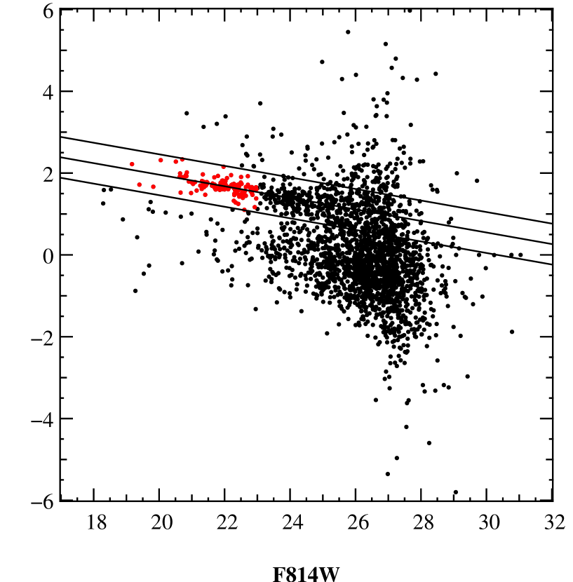
Figure 1: The red sequence of galaxy clusters in the F475W$-$F850LP, F814W colour-magnitude diagram. The galaxies that are included in the mass model are marked with red circles and have F475W$-$F850LP colour within 0.5 magnitudes from the mean of the red sequence.

The profiles of the cluster galaxies are based on a truncated isothermal sphere profile (Brainerd et al. 1996). The profile is characterised by a velocity dispersion $\sigma$ and a truncation radius $s$. The 3 dimensional mass density of a truncated isothermal sphere is given by:

$$\rho_{\mathrm{bbs}}(r)=\frac{\sigma^{2}}{2\pi Gr^{2}}\frac{s^{2}}{r^{2}+s^{2}}.$$ (1)

The galaxy haloes can be elliptical with the ellipticity implemented following the method presented in (Golse & Kneib 2002). All the galaxies included are treated in exactly the same way. This includes also the two massive central galaxies and the galaxies near multiple images.

The velocity dispersions of the galaxies are estimated from their F814W magnitude using the Faber-Jackson relation. Since we have been unable to find a good reference point to a fundamental plane or a Faber-Jackson relation at the redshift of the cluster we have used the fundamental plane known for the galaxy clusters A2218 and A2390 (Ziegler et al. 2001; Fritz et al. 2005) at redshifts 0.18 and 0.23 respectively. These same clusters were used as reference points when estimating the velocity dispersions of the galaxies in A1689 in Halkola et al. (2006). To model the galaxies in RX J1347 we have taken a model spectrum of an early type elliptical galaxy with a formation redshift of 5 from Bruzual & Charlot (2003), and passively evolved it from the redshift of RX J1347 ($z=0.451$) to 0.2. This model is used to calculate both the K-correction from the observed F814W to the F775W of the Faber-Jackson relation shown in Halkola et al. (2006) for clusters at redshift 0.2, and the evolution of the galaxy colours. The measured F814W magnitudes are corrected for galactic extinction according to Schlegel et al. (1998) obtained using the NASA/IPAC Extragalactic Database (NED).

We assume a linear relation between the truncation radius $s$ of a galaxy and its velocity dispersion $\sigma$. This is expected on theoretical grounds (Merritt 1983). Recently this topic has also been investigated using simulations that take into account the effect of baryons by Limousin et al. (2007b). These N-body simulations were done in order to study the tidal stripping of dark matter haloes of galaxies in a cluster, including star formation so that the stellar components of the galaxies can be followed. The simulations agree with trends observed using galaxy-galaxy lensing in galaxy clusters, e.g. Natarajan et al. (2002); Limousin et al. (2007a). It was additionally shown in Halkola et al. (2007) that for the strong lensing analysis of Abell 1689 (which has much stronger constraints on the mass from the multiple image systems identified in the cluster) it was not possible to constrain the slope of the power-law relation between $s$ and $\sigma$. Since the multiple images in RX J1347 do not constrain the sizes of the galaxies significantly we assume the same truncation law for the galaxies in RX J1347 as was found for galaxies in the galaxy cluster A1689 (Halkola et al. 2007) as the clusters are both similarly massive.

3.1.2 Smooth cluster mass

The X-ray measurements as well as the combined strong and weak lensing analysis of the cluster indicate that there is possibly a mass extension to the south-east of the cluster centre. The mass maps are otherwise fairly smooth and we therefore model the smooth mass component of the cluster with two parametric profiles. The second halo is also necessary in order to accurately reproduce the multiple images observed. Using parametric haloes to reconstruct the mass of galaxy clusters, as opposed to pixelated mass reconstructions for example, have several advantages but also disadvantages. The simple description of the mass distribution gives generally very good convergence properties when optimising the model parameters. On the other hand the mass profile is also relatively restricted in the mass distributions that can be recovered. Although the second halo could in principle be connected to a physical structure in the cluster, it is also possible that a secondary halo is necessary in the modelling in order to accurately model the mass distribution of the cluster with only one distinct halo. These two haloes are both described by either Navarro-Frenk-White (NFW Navarro et al. 1997) or by non-singular isothermal ellipsoid (NSIE) haloes.

The NFW halo is a prediction of cosmological numerical simulations and its 3-dimensional mass density is given by

$$\rho_{\rm{nfw}}(r)=\frac{\rho_{\rm{c}}}{(r/r_{\rm{s}})(1+r/r_{\rm{s}})^{2}},$$ (2)

where $\rho_{\rm{c}}$ is the characteristic density of the cluster and $r_{\rm{s}}$ is the scale radius which marks the transition from $\rho\propto r^{-1}$ to $\rho\propto r^{-3}$.

The NSIE profile is based on the popular isothermal sphere profile with the inclusion of a constant density core. The 3 dimensional mass density of the NSIE profile is given by

$$\rho_{\rm{nsie}}(r)=\frac{\sigma^{2}}{2\pi G}\frac{1}{(r^{2}+r_{\rm{c}}^{2})},$$ (3)

where $\sigma$ is the velocity dispersion of the isothermal sphere and $r_{\rm{c}}$ is the core radius of the sphere.

Both mass profiles have 6 free parameters: their position on the sky ($\alpha$, $\delta$), the ratio of their semi-minor and semi-major axes $r=b/a$, the position angle $\theta$, and the two parameters described above that define the density profile.

3.2 Multiple images

In the literature there are several published multiple image candidates in RX J1347 (e.g. Sahu et al. 1998; Bradač et al. 2005). In addition to these we have identified several new ones in the HST ACS images of the cluster, bringing the total number of candidate lensing system to 13. The images are shown in Fig. 2 and some of their properties are shown in Tab. 3 and thumbnail images in Figs. 13 - 18 of the appendix. The more tentative image candidates in a system are marked with a question mark in Tab. 3 and Fig. 2. The following sections discuss the multiple image systems in some detail.

The main analysis in this paper is based on image systems 1 and 2 only. The locations of the 5 images in image system 1 provide strong constraints on the distribution of mass in the cluster while the spectroscopic redshift of image system 2 is important in fixing the total mass scale. In section 5.4 we repeat the analysis with all image systems to check the effect of including all of them, and to obtain lensing redshift probability distributions for the image systems.

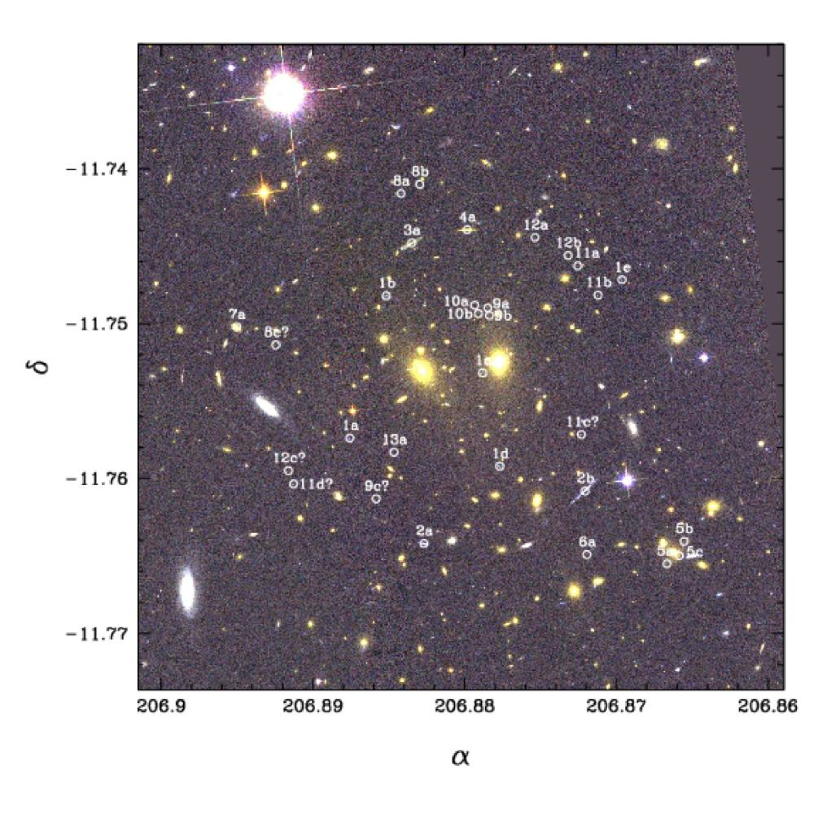
Figure 2: The multiple image systems identified in RX J1347$-$1145 overlaid on a colour image of the cluster made from the images taken with the ACS in filter F475W, F814W, and F850LP. The box size is $\sim$880 kpc, north is up, east is left. Uncertain image candidates are marked with a question mark. Only image systems 1 and 2 considerably constrain the mass profile of the cluster.

3.2.1 Image system 1

This is a multiple image system with 5 images on 4 sides of the cluster and a central image. The identification is based on the similar colours and morphology of the images, all images have a brighter knot at one end. Also the photometric redshift probability distributions of the multiple images in this system are very similar. They are flat and fairly broad and place the multiple image system in a redshift range 0.5-2.0. The M_F475W $-$ M_F814W and M_F814W $-$ M_F850LP colours of the multiple images are also in good agreement. We have obtained spectra for all the multiple images, but have not been able to identify any emission lines in the individual spectra. The many skylines in the spectra also hinder us from cross correlating the individual spectra to confirm the compatibility of the spectra of the multiple images. This mean that we cannot confirm the multiple image nature of the source from the spectra. Although the redshift cannot be fixed, the geometry of the images provide significant constraints on the mass profile.

3.2.2 Image system 2

Our image system 2 is composed of two images. The brighter of the two arcs was already identified by Schindler et al. (1995) as the south-west arc. The fainter arc was later found by Sahu et al. (1998). We have taken spectra of the two arcs and obtained a redshift of z_spec = 1.75 for the two of them; for more details see Lombardi et al. (2008, in prep.). The redshifts of the images fixes the overall mass scale of the cluster and provides strong support for them being multiple images. In Bradač et al. (2005) these correspond to images A4 and A5. Our models do not predict any additional detectable images for this system.

3.2.3 Image system 3

Image system 3 consists of only one distorted image. The spectroscopic redshift is z_spec = 0.806 (Ravindranath & Ho 2002), so this galaxy is a background galaxy and must be lensed. In the absence of counter images it cannot be effectively used to constrain the mass profile. Also the lack of multiple images can constrain the mass distribution, see Jullo et al. (2007). This is only effective if the singly lensed images are relatively close to critical regions so that multiple images are formed for model parameters that fulfill the other constraints reasonably well. In our analysis we have only afterwards checked that no additional images for this system are predicted.

3.2.4 Image system 4

Similarly to image system 3 this one consists of only one distorted image and therefore cannot effectively be used to constrain the mass model. The spectroscopic redshift of this galaxy is z_spec = 0.785 (Ravindranath & Ho 2002). No additional images for this system are predicted.

3.2.5 Image system 5

This image system consists of 3 faint images that are split by a cluster galaxy. The images are very sensitive to the mass in the galaxy which can therefore influence the total mass distribution significantly when this image system is included in the analysis.

3.2.6 Image system 6

A faint thin arc at a cluster centric radius of $\sim$12” larger than image system 2, and hence expected to be at a higher redshift. No counter images found. This is image system C in Bradač et al. (2005).

3.2.7 Image system 7

An arc that nicely bends around the galaxy at $\alpha$=13:47:34.8, $\delta$=$-$11:45:01.5. The exact shape of the arc is sensitive to the mass of the galaxy.

3.2.8 Image system 8

This is a 2-image system merging on a tangential critical line, also identified in Bradač et al. (2005) as a possible arc candidate. There is a tentative third image on the east side of the cluster but a positive identification is difficult due to the faintness of the source.

3.2.9 Image system 9

2 images merging on a radial critical line. We have identified a possible third image in the south-east part of the cluster.

3.2.10 Image system 10

A similar merging of 2 images at a radial critical line, close to image system 9. This one is much fainter though and less prominent and consequently less certain. A third image is expected near the third image of image system 9 but as this source is significantly fainter we have not identified one.

3.2.11 Image systems 11 and 12

In the north-west of the cluster there are several images that define a tangential critical line. The colours and morphology of the images vary, suggesting that the images originate from several different sources at a similar redshift. Possible counter images on the south-east and south west sides of the cluster are identified for system 11. The fainter image system 12 is more challenging in this respect although several candidates have been identified. In Bradač et al. (2005) identified as D1-D4.

3.2.12 Image system 13

A bluish galaxy oriented tangentially with respect to the cluster centre. It is potentially lensed although we have not been able to identify any counter images to this one.

4 Estimating the cluster mass distribution and its error

In order to estimate the mass distribution of the cluster we use Bayesian statistics with Markov chain Monte Carlo methods to estimate the probability distribution function of the free parameters of the cluster mass model.

Our mass models have 13 free parameters in total, the redshift of multiple image system 1 and 2$\times$6 parameters for the 2 smooth haloes for the global mass distribution.

4.0.1 Model $\chi^{2}$

Both the positional information as well as the relative magnifications of the images in an image system are used in calculating the $\chi^{2}$ for the models. The $\chi^{2}$ is given by

$$\chi^{2}=\sum_{i=1}^{N}\sum_{j=1}^{n_{i}}\frac{|\ \@vec{\beta}_{i,j}\ -\ \langle\@vec{\beta}\rangle_{i}|^{2}}{(\sigma_{i,j}/\sqrt{\mu_{i,j}})^{2}}+\sum_{i=1}^{N}\sum_{j=2}^{n_{i}}\frac{(\ f_{i,1}/\mu_{i,1}-f_{i,j}/\mu_{i,j}\ )^{2}}{(e_{i,1}/\mu_{i,1})^{2}+(e_{i,j}/\mu_{i,j})^{2}}.$$ (4)

In equation 4, $N$ is the number of multiple image systems, $n_{i}$ the number of images in system $i$ and $\@vec{\beta}_{i,j}$ denotes the source position of image $j$ in image system $i$, $\mu_{i,j}$ is the model magnification at the image position. $f_{i,j}$ and $e_{i,j}$ represent the isophotal flux and its estimated error of image $j$ in image system $i$. The first double summation in equation 4 therefore represents the scatter of the source positions weighted by the model magnification. The errors are assumed to scale with the square root of the magnification since the magnification is given by the ratio of an area of the image in the image plane to that of the unlensed image in the source plane. It was shown in Halkola et al. (2006) that this is a good estimate for the $\chi^{2}$ calculated in the image plane. The second double summation includes the relative magnifications between the images of an image system in the modelling. This is calculated by comparing the unlensed source fluxes of the multiple images. We use the first multiple image in each system as a flux reference.

4.0.2 Bayesian statistics

Bayes’ theorem deals with conditional probability distributions. We are specifically interested in constraining a model with parameters $w$ given data $d$ (and possibly some other prior knowledge of the system). The probability of a parameter set $w$ given the data $d$ can be written as

$$P(w|d)=\frac{P(d|w)P(w)}{P(d)},$$ (5)

where $P(d|w)$ is the probability of the data $d$ given the parameters $w$, $P(w)$ is the prior on the parameters $w$ and $P(d)$ is the probability of obtaining the data in the first place, also known as evidence. $P(d|w)$ is measured by the $\chi^{2}$ of our models and we will assume that it is proportional to $\rm{exp}(-\chi^{2}/2)$. We assume flat priors $P(w)$ for the parameters that are reasonable for DM haloes of galaxy clusters. $P(d)$ is treated as a normalising constant. With these simplifying assumptions it only remains to estimate $P(w|d)$. We do this with a Markov chain Monte Carlo method described below.

4.0.3 Markov chain Monte Carlo

The Markov chain Monte Carlo method is a popular way to estimate the errors in model parameters. It allows one to estimate the conditional probability distribution of parameters by statistically sampling the parameter space. In the Metropolis-Hasting algorithm the parameter space is explored in a random walk. It is a rejection sampling algorithm which means that the next set of random parameters is accepted with a probability that depends only on the difference in probability between successive sets of parameters. Given parameter sets $w_{i}$ with $\chi^{2}(w_{i})$ and a new perturbed parameter set $w_{i+1}$ with $\chi^{2}(w_{i+1})$ the probability $p$ of accepting the new parameter set $w_{i+1}$ is given by the ratio of the likelihoods of the parameter sets:

$$2\ \ln(\,p\,)=\left\{\begin{array}[]{ll}\chi^{2}(w_{i})-\chi^{2}(w_{i+1})&,\ \ for\ \chi^{2}(w_{i+1})>\chi^{2}(w_{i})\\ 0&,\ \ for\ \chi^{2}(w_{i+1})\leq\chi^{2}(w_{i})\\ \end{array}\right..$$ (6)

The new perturbed parameter sets $w_{i+1}$ are generated by random selection from Gaussian distributions centred on the individual parameters in $w_{i}$, and the widths of the Gaussian distributions are matched so that when each parameter is varied individually the effect on the acceptance rates converge to the same value of $\sim$60%. In the end all the widths are scaled so that an acceptance rate of $\sim$60% is achieved also when all the parameters are varied simultaneously. Another possibility would be to assume that the width is given by the error in the parameters. This would however require prior knowledge on the errors of the parameters. By tuning the widths according to the acceptance rate we ensure that all free parameters of the model have the same weight in the Markov chain. The acceptance rate of 60% is chosen as a compromise between denser local sampling of the parameter space at the cost of poorer global sampling (smaller width, higher acceptance rate), and an attempt to sample quickly a large volume of the parameter space that is hindered by low acceptance.

Each Markov chain is started with a mass model that has mass only in the galaxies. The two haloes describing the smooth mass component are set to be circular and to have no mass ($\sigma$ = 0 km/s for the NSIE profiles, and $\rho_{c}$ = 0 M${}_{\odot}/\rm{kpc}^{3}$ for the ENFW profiles). The two haloes are placed between the two bright central galaxies.

The Markov chains have a total length of 250 000. After the first $\sim$10 000 parameter sets $w_{i}$, the acceptance rate has stabilised at 60% as well as the scatter in the $\chi^{2}$ values for the parameter sets has stabilised. Although a ‘burning in’ of a Markov chain is strictly not necessary, we discard the first 10 000 parameter sets as these still show some memory on the initial conditions where haloes had no mass.

Each Markov chain has a fixed description for the mass in the galaxies. This means that individual Markov chains do not take into account the uncertainties of the velocity dispersion estimates of the galaxies. In order to account also for these uncertainties we calculate a total of 200 Markov chains where each has a different realisation of the galaxy component. In each Markov chain we have reassigned galaxy velocity dispersions from a Gaussian distribution centred on the measured value and with a width corresponding to the estimated error. Half of the Markov chains have a smooth component described by NSIE haloes and the other half by ENFW haloes.

All the remaining analysis is performed by combining the 200 Markov chains and randomly selecting 1000 parameter sets (with replacement) from the combined chain.

5 Results

The multiple images are reproduced well both in position and in morphology, although the mean separation between the observed image position and that predicted by the models is still well above the accuracy with which positions of galaxies can be measured. The mean separation in the MCMC analysis is $\sim 1^{\prime\prime}$ (for reference, the mean separation between an observed image position and that predicted by the models is $\sim 3.5^{\prime\prime}$ when the smooth mass component is described with only one halo). For comparison, the best models have separations below $\sim 0.5^{\prime\prime}$. Observed and predicted morphologies of the images can be seen in Figs. 13 and 14 in the appendix, where a discussion can also be found.

We explore the mass distribution of the cluster in two different ways. First of all we can study the parameter space of the smooth mass component. Secondly, we look at the total 2-dimensional mass distribution of the cluster as well as the averaged radial mass profile.

5.1 Parameters of the mass smooth component

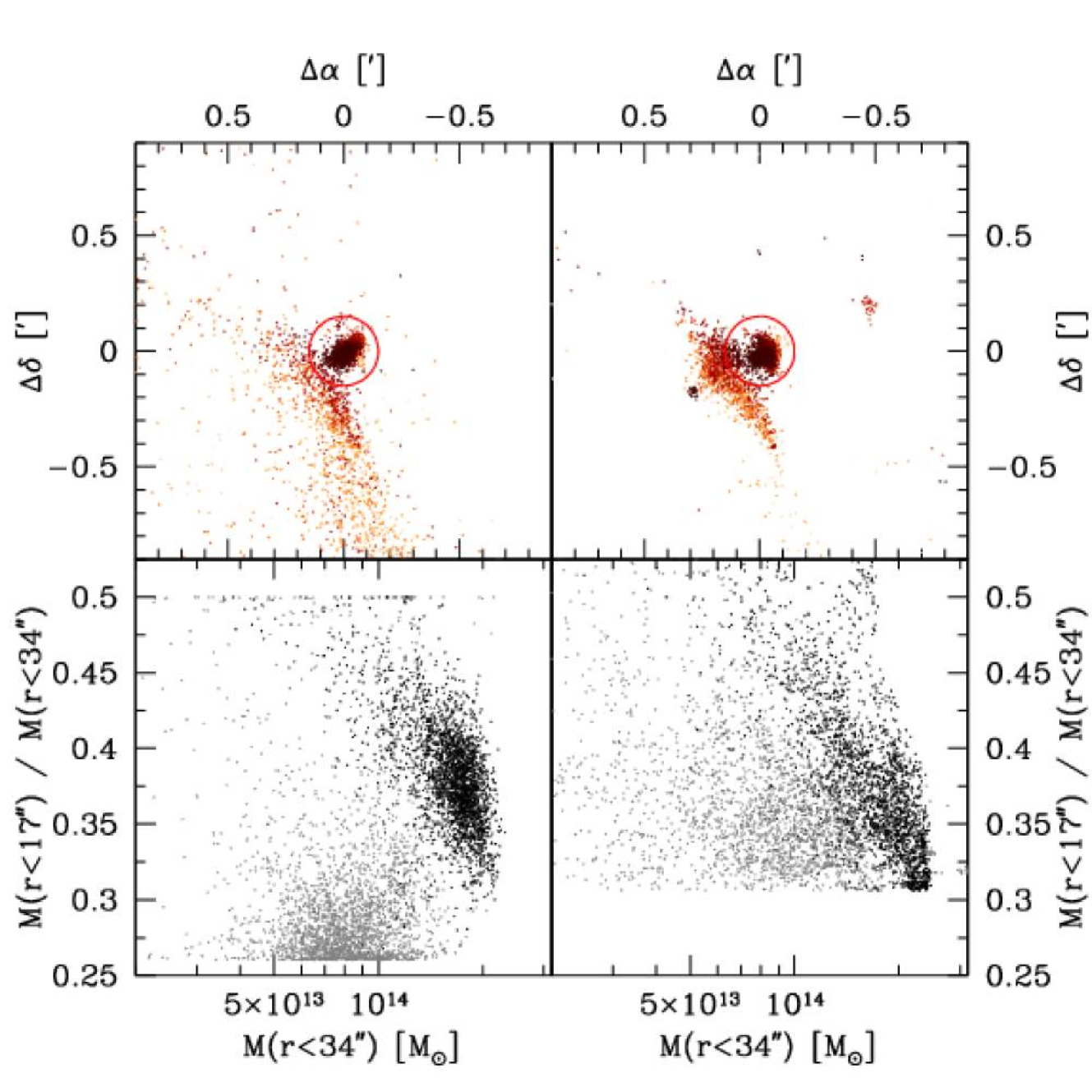
Figure 3: The distribution of the positions of the two smooth haloes in the MCMC sampling are shown on the two top panels, the NSIE profiles are on the left and the ENFW haloes on the right. One of the haloes resides preferentially in a relatively small region of the cluster centre, indicated by the red circle. This allows us to make a separation between the primary halo (within the circle) and the secondary halo (outside the circle). The points are coloured according to the mass of the haloes. The smaller haloes with $\rm{M(r<34^{\prime\prime})<5\times 10^{13}M_{\odot}}$ are light orange in colour and the massive haloes with $\rm{M(r<34^{\prime\prime})>2\times 10^{14}M_{\odot}}$ are coloured black. In the bottom panels we plot the concentration as measured by the ratio of the halo mass at two different radii, $\rm{M(r<17^{\prime\prime})}/\rm{M(r<34^{\prime\prime})}$, against the mass within the Einstein radius of the cluster, $M(r<34^{\prime\prime})$. The primary haloes (black) are generally both more massive and more concentrated then the corresponding secondary haloes (grey). The separation is clear for the NSIE haloes, where as the concentration of the ENFW profiles are the same for both the primary and secondary haloes. The positions on the upper panels are relative to $\alpha$ = 13:47:30.9, $\delta$ = $-$11:45:08.6, the centre of the circle.

The distribution of the positions of the smooth DM haloes in the MCMC analusis are shown in the two top panels in Fig. 3. The left panels are for the NSIE halos and the right panels for the ENFW haloes. We have used the positions of the haloes to separate the primary and secondary haloes. The primary halo is defined as the one whose centroid lies within the red circle shown in the top panels. In a small number of cases both the primary and the secondary halo reside either inside or outside the red circle. In these cases we have taken the halo with a larger $M(r<34^{\prime\prime})$ as the primary halo. The points are coloured according to the mass of the haloes with smaller haloes, $M(r<34^{\prime\prime})<5\times 10^{13}M_{\odot}$, being light orange and massive haloes, $M(r<34^{\prime\prime})>2\times 10^{14}M_{\odot}$, being black. It is clear from the plot that the central haloes are also the more massive ones, and that the less massive haloes populate the outer regions of the cluster centre.

The more massive haloes are spatially concentrated in a very small region for both the NSIE and ENFW profiles. The less massive ones are more spread out for both profiles, although the NSIE profiles are more scattered than those described by ENFW profiles.

In order to be able to compare the masses and concentrations of the NSIE and ENFW haloes we calculate the mass of the haloes at two different radii ${r_{1}}$ and ${r_{2}}$, where ${r_{1}}<{r_{2}}$. We can then define concentration ${c_{m}}$ as the ratio of the two masses ${c_{m}}={M(r<r_{1})}\ /\ {M(r<r_{2})}={M_{1}}\ /\ {M_{2}}$. If all the mass is already contained within ${r_{1}}$ then the mass ratio is 1, where as for a mass sheet the ratio is given by $({r_{1}}/{r_{2}})^{2}$. For a singular isothermal sphere the maximum value for ${c_{m}}$ is $({r_{1}}/{r_{2}})$, since ${M(r)}\propto r$. The outer radius ${r_{2}}$ is taken to be 34 arcseconds which corresponds roughly to Einstein radius of the cluster, while the inner radius is arbitrarily defined as ${r_{1}}={r_{2}}/2$. The separation in concentration and mass is not very sensitive to the chosen radii, ${r_{1}}$ and ${r_{2}}$. On the bottom panels of Fig. 3 we plot the concentration ${c_{m}}$ against ${M(r<34^{\prime\prime})}$ for the NSIE (left) and the ENFW (right) haloes. The primary haloes are coloured black, while the secondary haloes are coloured grey. For the NSIE profiles the separation between the primary and secondary haloes in the ${c_{m}}$ vs. ${M(r<34^{\prime\prime})}$ space is clear with primary haloes being both more massive and more concentrated with a mean mass of ${M(r<34^{\prime\prime})}$ = ( 16.1 $\pm$ 3.3 ) $\times$ $10^{13}$ ${M_{\odot}}$ and a mean concentration of ${c_{m}}$ = 0.38 $\pm$ 0.04 compared to the secondary haloes which have a mean mass of ${M(r<34^{\prime\prime})}$ = ( 8.9 $\pm$ 2.8 ) $\times$ $10^{13}$ ${M_{\odot}}$ and a mean concentration of ${c_{m}}$ = 0.30 $\pm$ 0.06. This separation is less pronounced for the ENFW profile where the concentrations are virtually same for the primary and the secondary haloes (${c_{m}}$ = 0.38 $\pm$ 0.06 vs. ${c_{m}}$ = 0.38 $\pm$ 0.11). The mean masses of the primary and the secondary haloes are ${M(r<34^{\prime\prime})}$ = ( 16.3 $\pm$ 5.0 ) $\times$ $10^{13}$ ${M_{\odot}}$ and ${M(r<34^{\prime\prime})}$ = ( 7.9 $\pm$ 5.4 ) $\times$ $10^{13}$ ${M_{\odot}}$ respectively. One should keep in mind that since the ENFW halo has always an inner logarithmic slope of $-1$, the profile can never reach as low a concentration as an NSIE profile can. This is also the reason why the positions of the secondary haloes for the ENFW profile have less scatter: the position of an ENFW halo is always well defined.

5.2 Total mass distribution of RX J1347$-$1145

Due to the large scatter in the parameters of the smooth mass distribution it is perhaps more interesting to look at the total 2-dimensional projected mass distribution of the cluster. The averaged 2-dimensional projected scaled mass distribution for a source at redshift 2 is shown in Fig. 4. Thick contours lines are used for $\kappa\leq 1$ levels, where as thin lines are used for $\kappa<1$ contours (the contours are separated by $\Delta\kappa$=0.25, the first thick contour level is at $\kappa$=1).

Figure 4: The average scaled surface mass density contours for a source at redshift 2. The thick contours show the $\kappa$ levels greater or equal to one, and the thin lines for $\kappa$ less than one (the contours are separated by $\Delta\kappa$=0.25, first thick contour level is at $\kappa$=1).

For each of the 1000 selected parameter sets from the MCMC analysis we have also calculated separately the contributions to the total mass from the galaxies and the smooth component. The radial mass profiles of the galaxy mass component and that of the total cluster mass are shown in Fig. 5. In the bottom panel the total mass (galaxies and the smooth mass component) are shown as crosses, and the mass in the galaxies as circles. The errors show the 1-sigma errors derived from the MCMC analysis. The error in the total mass is very small at ${r}\sim 35^{\prime\prime}$ where the mass is fixed by the spectroscopic redshift of image system 2.

Figure 5: Mass profile of RX J1347. In the bottom panel we show the mass in the galaxies as circles and the total mass as crosses. The error bars show the 68% confidence interval derived from the MCMC analysis. The top panel shows the residual mass needed to perfectly reproduce the image positions as a percentage of the total mass. It is consistent with 0% at all radii.

We can estimate the NSIS and NFW parameters of the total mass distribution by fitting a single halo to the total radial mass profile. The 1-, 2- and 3-sigma contours for the NSIS and NFW parameters are shown in Figs. 6 and 7 respectively. We also plot in the figures the error bars for the individual parameters when marginalised over the other parameter. The best fit parameters of the NSIS profile are $\sigma$=1949 ${}_{-39}^{+40}$ km/s, and $r_{\rm{c}}$=20.3 ${}_{-1.8}^{+1.8}$ ”. The velocity dispersion is high due to the presence of a large core. The NFW profile parameters are $r_{200}$ = 3.3 $\pm$ 0.2 Mpc, and $c$ = 5.4 ${}_{-0.5}^{+0.7}$. The $\chi^{2}$ values for both of the profiles are very good (for 14 degrees of freedom $\chi^{2}$ values of 4.5 and 4.2 are obtained for NSIS and NFW profiles respectively). The very good $\chi^{2}$ values probably reflect the way the total mass profile was obtained using haloes that had NSIE and ENFW profiles.

Figure 6: The 1-, 2- and 3-$\sigma$ confidence regions for a NSIS halo fitted to the total mass. The point with error bar shows the best fit value and the marginalised 1-sigma errors for the two parameters. The best fit parameters are $\sigma$=1949 ${}_{-39}^{+40}$ km/s, and $r_{\rm{c}}$=20.3 ${}_{-1.8}^{+1.8}$ ^′′.

Figure 7: The 1-, 2- and 3-$\sigma$ confidence regions for an NFW halo fitted to the total mass. The point with error bar shows the best fit value and the marginalised 1-sigma errors for the two parameters. The best fit parameters are $r_{200}$ = 3.3 $\pm$ 0.2 Mpc, and $c$ = 5.4 ${}_{-0.5}^{+0.7}$.

5.2.1 RX J1347$-$1145 as a merger

It is clear from the surface mass density contours that the mass distribution of the cluster does not have any evident bimodality, although two haloes were used in modelling the mass. If the cluster was undergoing a merger along the line of sight, this could still require two haloes in the modelling. The fairly clean separation of the two haloes in both mass and concentration as well as to a lesser extent also in position, if taken seriously, would indicate that RX J1347 is a merger with a 2:1 mass ratio of the merger progenitors. This supports well the results from both X-rays (e.g. Allen et al. 2002) and SZ-effect (e.g. Komatsu et al. 2001) that find X-ray shocks and complicated substructure in the cluster. This was also seen in a combined strong and weak lensing analysis by Bradač et al. (2005). Although the 2-dimensional mass map obtaned here does not have a clear peak in the south-east part of the cluster where the X-ray and SZ structures are seen, it is worth noting that it is also in this part of the cluster where the second halo is preferentially located.

We have added a third halo to the smooth mass component but have not been able recover the south-east extension. The strong lensing constraints in this part of the cluster are weak due to the lack of multiple images in this region, and affects our ability to determine the mass distribution accurately. This includes the position of the secondary halo.

Interestingly the cluster has a very low velocity dispersion of only 910$\pm$130 km/s measured by Cohen & Kneib (2002). They discussed that this could be explained if the merger took place perpendicular to the line of sight and therefore would have increased the velocity dispersion mostly in that direction.

It is important to keep in mind that in the strong lensing analysis presented here we assume that the cluster has two haloes. More work is necessary in order to establish with more confidence that the two haloes in our modelling do correspond to physical haloes. It is also possible that the need for two haloes in the modelling has to do less with physically separated structures in the cluster than with a complex morphology of one dominant halo. This could be, for example, a varying ellipticity (both magnitude and position angle) as a function of cluster centric radius, slightly asymmetric mass profile, or a mass profile that is neither an ENFW nor an NSIE profile but can be modelled as a superposition of two such haloes.

5.2.2 Residual mass maps

We have taken inspiration from LensPerfect by Dan Coe that, as its name implies, allows one to find a mass distribution that exactly reproduces all multiple image positions. We have implemented a similar scheme with the intention to check how our parametric mass profile needs to be modified in order to exactly reproduce the image positions. The usual parametric modelling is used as a basis after which we calculate residual mass map needed for a perfect fit. In calculating the residual mass maps we have not considered the relative magnifications of the multiple images but only their positions.

In practice the residual mass map is found by calculating the residual deflection angle $\Delta\@vec{\alpha}(\@vec{\theta}_{i,j})$ at each multiple image position $\@vec{\theta}_{i,j}$:

$$\Delta\@vec{\alpha}(\@vec{\theta}_{i,j})=\ \@vec{\beta}_{i,j}-\langle\@vec{\beta}\rangle_{i},$$ (7)

where $\@vec{\beta}_{i,j}$ is the source position of image $j$ in system $i$ as obtained with the parametrised model and $\langle\@vec{\beta}\rangle_{i}$ is the mean source position of the images in system $i$.

The residual deflection angle $\Delta\@vec{\alpha}(\@vec{\theta})$ at any other point is then calculated using a Thin Plate Spline interpolation (TPS, for details on the topic see e.g. Bookstein 1989). The interpolated surface has the property that it minimises the bending energy of the function $\Delta\@vec{\alpha}(\@vec{\theta})$ ,

$$E=\int\!\!\int\Bigg{[}\frac{\partial^{2}\Delta\@vec{\alpha}}{\partial\theta_{1}^{2}}+2\ \Bigg{(}\frac{\partial^{2}\Delta\@vec{\alpha}}{\partial\theta_{1}\partial\theta_{2}}\Bigg{)}^{2}+\frac{\partial^{2}\Delta\@vec{\alpha}}{\partial\theta_{2}^{2}}\ \Bigg{]}\ \mathrm{d}\theta_{1}\mathrm{d}\theta_{2},$$ (8)

where $\theta_{1}$ and $\theta_{2}$ are the Cartesian components of the position vector $\@vec{\theta}$.

The amount and location of residual mass $\Delta\kappa(\@vec{\theta})$ that is needed to perfectly reproduce the multiple image positions is then simply calculated from the residual deflection angle. Since the surface mass density is related to the deflection angle via $\kappa=\@vec{\nabla}\@vec{\alpha}/2$, the use of TPS interpolation essentially minimises the gradients of $\Delta\kappa$.

The 2-dimensional distribution of the residual mass $\Delta\kappa$ is shown in Fig. 8. The red and blue contours show positive and negative contributions, respectively, while the white line shows the $\Delta\kappa=0$ level. The very small correction needed is represented by the very small separation of the contours of only 0.005. Although the correction to the mass is small, it is clear from Fig. 8 that the correction has a bipolar distribution so that south-east and north-west quadrants have generally a mass deficit in the parametric modelling while the south-west and north-east quadrants have a slight mass surplus.

The radial mass profile of the residual mass map is shown on the top panel in Fig. 5 as a percentage of the total mass at any given radius. In the strong lensing region of the cluster the average residual mass at any radius is consistent with 0% with a scatter of only around 1%.

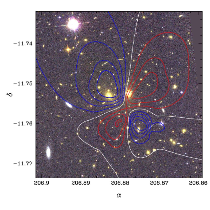
Figure 8: The residual surface mass density contours for a source at redshift 2. The red and blue contours show positive and negative contributions respectively while the white line shows the $\Delta\kappa=0$ level. The contours are separated by 0.005 in $\kappa$ indicating that only a very small correction to the mass map is enough to perfectly reproduce the multiple image positions.

5.3 Lensing redshift of multiple image system 1

The lensing models allow us to also constrain the redshifts of multiple image systems. This can be done by looking at the distribution of the redshifts of the multiple image systems in the MCMC sampling of the parameter space. The redshift probability density of multiple image system 1 is shown in Fig. 9. The dotted line shows the redshift distribution from the lensing and the dot-dashed from the photometric redshift analysis, while the solid line shows the total distribution. The lensing redshift distributions do not show any dependence on the profile used in modelling the smooth mass component of the cluster. The lensing redshift for image system 1 is z_lens=1.90${}^{+0.21}_{-0.31}$. The photometric redshift was not used as a prior in the lensing modelling, and we only use it to compare to the redshift obtained with the lensing models. The two estimates for the source redshift agree in the redshift range 1.5-2.0 with a combined mean redshift of 1.70${}^{+0.13}_{-0.12}$.

Figure 9: The redshift distribution of image system 1 in the MCMC sampling of the parameter space. The dotted line shows the lensing redshift probability distribution. The photometric redshift probability distrubution is given by the dot$-$dashed line. Combining the two probability densities results in the solid line. The lensing redshift probability densities have a clear cutoffs at $z\sim 1.5$ and $z\sim 2.5$. The lensing redshift for image system 1 is $z_{\mathrm{lens}}$=1.90${}^{+0.21}_{-0.31}$, with the best combined estimate being 1.70${}^{+0.13}_{-0.12}$.

5.4 Constraints from all multiple image systems

All the previous analysis has been based on models that use only image systems 1 and 2 to constrain the mass distribution of the cluster. We have repeated the analysis using all multiple image systems to check how the mass distribution changes in the presence of more constraints, and to predict redshifts for the remaining multiple image systems. The source redshifts are added as free parameters to the models without priors from photometric redshifts.

5.4.1 Mass distribution

The mass distribution obtained with all the multiple images are virtually indistinguishable from that obtained with only the two first ones. The surface mass density contours for the mass distribution derived with constraints from all multiple images systems are shown in Fig. 10. The contour levels are the same as those used in Fig. 4. The differences are most noticeable around some of the cluster galaxies. Also the critical lines are only marginally affected when all image systems are used.

The reason for the similarity of the mass maps is most likely the free redshifts of the multiple images combined with the geometry of the images. With the exception of image systems 9 and 11 all of the image systems are only on one side of the cluster. The unconstrained redshifts leave the mass scale free while the geometries cannot constrain the position of the mass concentration. All of the information is hence contained in the first two image systems which constrain the position of the mass concentration through the 5 images in image system 1 while the scale is fixed by the spectroscopic redshift of image system 2.

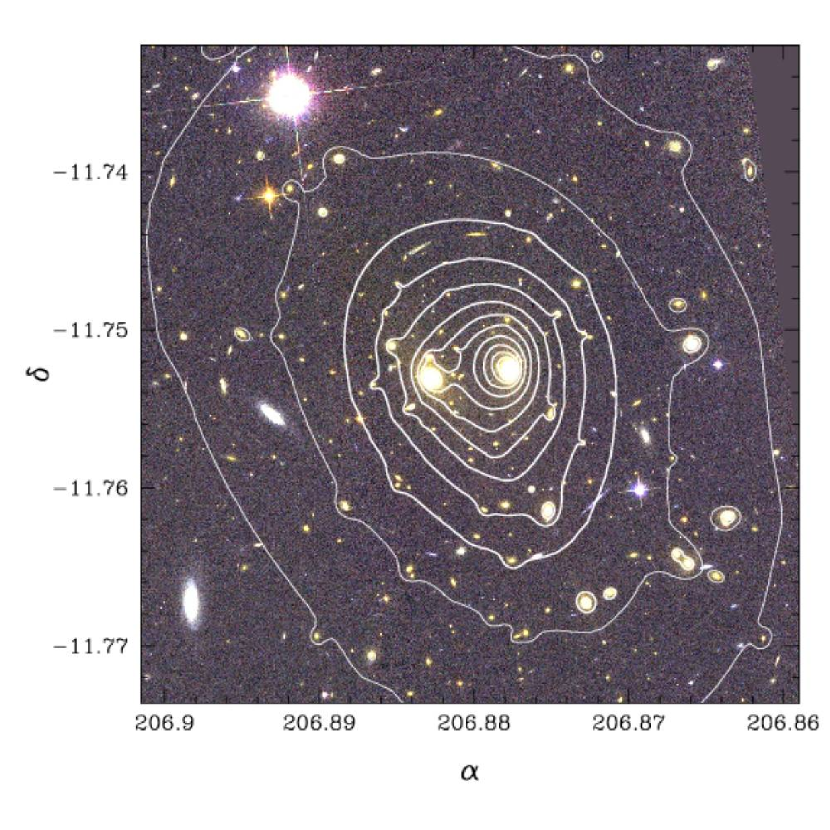
Figure 10: The average scaled surface mass density contours for a source at redshift 2. All image systems were used to constrain the mass distribution. The thick contours show the $\kappa$ levels greater or equal to one, and the thin lines for $\kappa$ less than one (the contours are separated by $\Delta\kappa$=0.25, first thick contour level is at $\kappa$=1), these are the same as in Fig. 4 for easier comparison. The differences are very small, mostly noticeable by small deviations near cluster galaxies.

5.4.2 Lensing redshifts of multiple image systems

The redshift probability densities for image systems 1, 6, 8, 9, 10, 11, and 12 are shown in Fig. 11 as dotted lines. The redshifts of the other multiple image systems are poorly constrained. The lower redshift bump on the probability densities for the image systems 9 and 10 is a consequence of their modelling. We have only required that a critical line should pass between the two images in these systems. For a source at low redshift it is the tangential critical line, and not the radial one, that passes through the two images. The dot-dashed line shows the probability distribution of the photometric redshifts, the solid line the probability density combining both the lensing and photometric redshifts probability densities. The photometric redshift probability distribution of image system 8 has two distinct peaks, one between 0.6 and 2.0 and another between redshifts 4 and 5. The lensing redshift probability distribution for this image system is broad but excludes the lower redshift bump seen in the photometric redshift probability distribution. The photometric redshift probability densities for the other image systems are very broad and constrain the redshifts very little. The low redshift bump in image systems 9 and 10 can be excluded since in those cases the image systems would define a tangential critical curve where as it is clear from the ACS images that the images are separated by a radial critical curve.

Figure 11: The redshift distributions of the image systems for which the lensing models are able to constrain the redshift. The dotted line shows the lensing redshift probability distribution, the dot-dashed line the photometric redshift probability distribution and the solid line the combined redshift probability distribution. All multiple images are used in the lensing modelling. For image systems 9 and 10 the model requirement is that a critical curve should pass between the two images. This produces the low redshift bump in the redshift probability when the tangential critical curve and not the radial critical curve passes between the two images. As it is clear from the positions of the multiple images that they form a radial arc, the lower redshifts can be ignored.

6 Comparison to previous mass estimates

There are several previous mass estimates for RX J1347$-$1145 in the literature. In this section we compare the masses from different methods, namely from the kinematics of the cluster galaxies, X-ray emission from the cluster gas, weak and strong lensing separately (WL & SL, analysis respectively) as well as a combined strong and weak lensing (SWL). We have converted results in the literature to the cosmology used in this work (H₀ = 70 km/s/Mpc, $\Omega_{\rm{m}}$=0.3 and $\Omega_{\Lambda}$=0.7), whenever required. For the direct mass comparison we have only used literature values where projected masses are given. The converted masses are shown in Table 1 and plotted in Fig. 12.

Figure 12: Projected mass profile of RX J1347 from various published results. The solid line shows the mass profile obtained in this work (the dashed lines show the 1-sigma confidence region in mass). The different symbols in the figure denote different methods, weak lensing (WL), strong lensing (SL), strong and weak lensing (SWL) and finally X-rays shown by filled circles, crosses, a triangle, and squares respectively (also labelled in the figure). The authors are marked next to the points, full details can be found in the text. We have plotted only X-ray masses where projected masses are given in literature.

The strong lensing mass estimate by Sahu et al. (1998, S98) is almost a factor of 4 higher than what we obtain. This is probably caused by the low redshift assumed for the arc by Sahu et al. (1998) and their assumption of spherical symmetry. The two purely weak lensing mass estimates have either higher (Kling et al. 2005, K05) or lower (Fischer & Tyson 1997, F97) masses than what we obtain with strong lensing. This indicates that there is at least no systematic offset between weak and strong lensing masses obtained.

The agreement with X-ray mass estimates by both Schindler et al. (1997, S97) and Gitti et al. (2007, G07) is fairly good, although all of the X-ray mass estimates are lower than the ones we obtain. A detailed comparison of lensing mass from a combined strong and weak lensing analysis to new X-ray data taken with the Chandra X-ray telescope is presented in Bradač et al. (2008, in preparation). We find excellent agreement with the combined strong and weak lensing analysis of Bradač et al. (2005, B05). This is not surprising since the redshift for the arc used both in Bradač et al. (2005) and this work has not changed, thus fixing the mass of the cluster at the position of the arc.

Table 1: Comparison of projected mass estimates interior to a given radius in the literature. The different methods are weak lensing (WL), strong lensing (SL), strong and weak lensing (SWL), X-rays and kinematics of the cluster galaxies. We have converted all the results to the cosmology used in the this paper (H₀ = 70 km/s/Mpc, $\Omega_{\rm{m}}$=0.3 and $\Omega_{\Lambda}$=0.7) if necessary. The remarks for Gitti et al. (2007) refer to the types of profiles fitted, SO for a single $\beta$ model and DDg1 for a double $\beta$ model.

Reference	$r$	M($<r$)		Method
	′′	1014 M⊙		(Remark)
Gitti et al. (2007)	35	2.	38 $\pm$ 0.27	X-ray (SO)
Gitti et al. (2007)	35	2.	05 $\pm$ 0.37	X-ray (DDg1)
Schindler et al. (1997)	35	2.	94	X-ray
Sahu et al. (1998)	35	8.	82	SL
This work	35	2.	56 $\pm$ 0.12	SL
Bradač et al. (2005)	89	8.	40 $\pm$ 2.10	SWL
This work	89	8.	57 $\pm$ 1.34	SL
Kling et al. (2005)	124	25.	20 $\pm$ 5.60	WL (SIS)
Kling et al. (2005)	124	29.	40 ${}_{-4.20}^{+2.80}$	WL (NFW)
This work	124	12.	60 $\pm$ 2.58	SL
Gitti et al. (2007)	147	9.	35 ${}_{-1.03}^{+1.05}$	X-ray (SO)
Gitti et al. (2007)	147	9.	17 $\pm$ 2.13	X-ray (DDg1)
Fischer & Tyson (1997)	294	11.	90 $\pm$ 2.80	WL

In cases where we have not found projected mass estimates for the cluster we can still compare our results for the parameters of the commonly used halo profiles, namely the family of isothermal profiles and the Navarro, Frenk and White profile. These are shown in Table 2. For the comparison we have converted the literature values of the $r_{\rm{c}}$ of an isothermal profile and the $r_{200}$ of an NFW profile to our cosmology where applicable. In addition, if only $r_{\rm{s}}$ of an NFW profile was given in the literature we have multiplied it (and its error) by the concentration parameter given to obtain an $r_{200}$. This is only a rough estimate of the error, however, since the two parameters have very strong degeneracies with higher concentrations having smaller scale radii.

The high core radius required to fit the mass profile in this work is compensated by an unusually high velocity dispersion. A singular isothermal sphere would have a much lower velocity dispersion (in the range 1450-1600 km/s) as can be seen at least qualitatively by extending the degeneracy of the two parameters in Fig. 6. The exact value obtained for the velocity dispersion depends very strongly on the range of radii in which the mass is fitted. On the other hand the range of velocity dispersions is in good agreement with the singular isothermal fits in the literature. This also includes the X-ray based velocity dispersion measurement by Allen et al. (2002), once the large core radius found in our analysis is taken into account (for a given velocity dispersion a larger core radius lowers the mass of an isothermal sphere).

The concentration parameter we obtain for the NFW profile is in agreement with the relatively low concentrations expected of cluster -sized haloes. The $r_{200}$ (3.3 $\pm$ 0.2 Mpc) on the other hand is rather large when compared to the literature. Since we are only determining the mass in the strong lensing regime we are not able to effectively constrain the mass at large radii, e.g. at the virial radius of the cluster, the value we obtain for $r_{200}$ is therefore an extrapolation of the NFW profile from the very inner regions of the cluster. In our case the scale radius NFW profile is already $\sim$600 kpc and outside the region that can be probed directly with strong lensing only. Weak lensing analysis beyond the field of view of the ACS is necessary to strongly constrain the $r_{200}$ of the cluster. This work will be done in Wuttke et al. (2008, in preparation) using both WFI and MegaCam data.

Table 2: Comparison between the estimated parameters of different parametrised mass profiles from the literature. When comparing parametrised halo profiles there is no confusion between spherical and cylindrical densities/masses making the comparison of different methods easier. We have converted the $r_{\rm{c}}$ of an isothermal profile and the $r_{200}$ of an NFW profile to our cosmology where applicable. If only $r_{\rm{s}}$ of an NFW profile was given in literature we have multiplied it (and its errors) by the best fit concentration to obtain an $r_{200}$.

Reference	$\sigma$		$r_{\rm{c}}$		Method
	km/s		kpc
Cohen & Kneib (2002)	910	$\pm$ 130			kinematic
Allen et al. (2002)	1590	$\pm$ 150	38	$\pm$ 8	X-ray
Kling et al. (2005)	1400	${}^{+130}_{-140}$			WL
Fischer & Tyson (1997)	1500	$\pm$ 160			WL
This work	1949	$\pm$ 40	117	$\pm$ 12	SL
Reference	$c$		$r_{200}$		Method
			Mpc
Allen et al. (2002)	5.87	$\pm$ 1.4	1.99	${}^{+1.19}_{-0.60}$	X-ray
Gitti et al. (2007)	3.2	$\pm$ 0.3	2.31	$\pm$ 0.36	X-ray
Kling et al. (2005)	15	${}^{+64}_{-10}$	2.64	${}^{+0.14}_{-0.57}$	WL
This work	5.4	${}_{-0.5}^{+0.7}$	3.29	$\pm$ 0.20	SL

7 Conclusion

In this paper we present the first detailed strong lensing model for the galaxy cluster RX J1347$-$1145 . The models are based on images taken with the Advanced Camera for Surveys on the Hubble Space Telescope. The high resolution of the image along with the three colours have allowed us to identify several new strongly lensed background images in the cluster. The follow-up spectroscopic observations on the FORS2 at the VLT have provided us with redshifts for the images in one multiple image system. This is crucial for an accurate absolute mass determination of the cluster. Among the new multiple image systems is a 5 image system with a central image that is very important in fixing the mass profile at the core of the cluster.

The mass in the cluster is modelled with small-scale mass components in the cluster galaxies described by truncated isothermal ellipsoids, and a large-scale component in two parametric mass profiles (Navarro, Frenk and White profile and non-singular isothermal ellipsoid). The parameters of the large-scale component are constrained by the location and magnifications of the multiple images. The total mass profile of the cluster is well described by both a Navarro, Frenk and White profile with a moderate concentration of $c$ = 5.3${}^{+0.4}_{-0.6}$ and $r_{\rm{200}}$ = 3.3${}^{+0.2}_{-0.1}$ Mpc, or a non-singular isothermal sphere with velocity dispersion $\sigma_{\rm{nsis}}$ = 1949 $\pm$ 40 km/s and a core radius $r_{\rm{c}}$ = 20.3 $\pm$ 1.8 ^′′. The core radius in the isothermal profile is necessary in order to reproduce the central image and to fit the total mass of the profile at the all radii. A singular isothermal sphere fit to the total mass has too much mass at small radii and too little at larger radii. The total mass of the cluster inside the Einstein radius of the main arc ($\sim 35^{\prime\prime}$, or $\sim$200 kpc) is (2.6 $\pm$ 0.12) $\times$ 10¹⁴ M_⊙.

A comparison with the X-ray mass estimates by Gitti et al. (2007) shows that the lensing mass is consistently higher than the X-ray mass, although still within the error bars. The X-ray based velocity dispersion in Allen et al. (2002) on the other hand is in good agreement with the one determined here once the effect of the different core radii is taken into account.

8 Acknowledgements

A. Halkola and T. Erben acknowledge support by the German BMBF through the Verbundforschung under grant no. 50 OR 0601. M. Bradač acknowledges support for this work provided by NASA through grant number HST-GO-10492.03A from the Space Telescope Science Institute, which is operated by AURA, Inc., under NASA contract NAS 5-26555. MB acknowledges support from the NSF grant AST-0206286 and from NASA through Hubble Fellowship grant # HST-HF-01206.01 awarded by the Space Telescope Science Institute.

This research has made use of the NASA/IPAC Extragalactic Database (NED) which is operated by the Jet Propulsion Laboratory, California Institute of Technology, under contract with the National Aeronautics and Space Administration.

Based on observations made with the NASA/ESA Hubble Space Telescope, obtained from the data archives at the Space Telescope European Coordinating Facility and the Space Telescope Science Institute, which is operated by the Association of Universities for Research in Astronomy, Inc., under NASA contract NAS 5-26555.

Appendix A Multiple image systems

The multiple images with some of their properties are listed in Table 3. The images in each image system are shown in Figs. 13-18. In addition we show for multiple image systems 1 and 2 the images and predicted images in Figs. 13 and 14. In the figures the top row shows the original 3-colour image created from the HST ACS images in F475W (blue), F814W (green) and F850LP (red) pass bands. The scales are shown on the images. The model prediction on the lower row are created by taking the first image of an image system, delensing it into the source plane using the lensing model and then relensing it back to the image plane at the positions of the multiple images. The first multiple image in each system is therefore reproduced exactly both in shape and position, while the remaining multiple images have an offset and a distortion relative to the observed multiple image due to the model. Note that this assumes that the source position of the multiple image system is at the source position of the first image, not the average source position which is used in calculating the $\chi^{2}$. The sizes and positions are matched well indicating that both the magnifications (size) and positions are well reproduced by the model. Image 1b has somewhat larger discrepancy both in magnification and position (the positional offset is 3^′′). This can be at least partly due to the presence of a cluster galaxy near the multiple image position. A comparison of the orientations of the model images with the observed ones (see Fig. 13) can be used to check the quality of the modelling since the orientations have not been used in determining the mass distribution. The orentations are in excellent agreement providing strong support for the mass modelling presented in this paper. The mean separation between an image in an image system and that of the models is $\sim 1^{\prime\prime}$ in the MCMC analysis. Note that this is relatively large since the MCMC chain does not explicitly try to minimise the $\chi^{2}$. The best models in the MCMC analysis have mean separations below $\sim 0.5^{\prime\prime}$.

Table 3: Positions, colours and redshifts estimates for the multiple images in this study. The mass profile and lensing redshifts are constrained by image systems 1 and 2 only. The more tentative images in a system are marked with a question mark.

Multiple	$\alpha$	$\delta$	MF475W - MF814W	MF814W - MF850LP	zspec	zphot
image	J2000	J2000
1a	13:47:33.009	$-$11:45:27.28	0.23 $\pm$ 0.03	$-$1.04 $\pm$ 0.05		-
1b	13:47:32.432	$-$11:44:54.23	0.12 $\pm$ 0.03	$-$1.11 $\pm$ 0.05		-
1c	13:47:30.906	$-$11:45:12.14	0.11 $\pm$ 0.06	$-$0.99 $\pm$ 0.09		-
1d	13:47:30.635	$-$11:45:33.84	0.15 $\pm$ 0.03	$-$1.10 $\pm$ 0.05		$2.19\pm 0.05$
1e	13:47:28.703	$-$11:44:50.54	0.22 $\pm$ 0.03	$-$1.06 $\pm$ 0.05		$2.20\pm 0.15$
2a	13:47:31.834	$-$11:45:51.80	0.24 $\pm$ 0.01	$-$1.00 $\pm$ 0.01	1.751	$0.01\pm 0.05$
2b	13:47:29.283	$-$11:45:39.59	0.17 $\pm$ 0.01	$-$1.00 $\pm$ 0.01	1.751	$0.01\pm 0.02$
3a	13:47:32.027	$-$11:44:41.98	1.39 $\pm$ 0.01	$-$0.95 $\pm$ 0.01	0.8062	$1.26\pm 0.02$
4a	13:47:31.148	$-$11:44:38.87	2.59 $\pm$ 0.03	$-$0.76 $\pm$ 0.01	0.7852	$1.32\pm 0.02$
5a	13:47:27.988	$-$11:45:56.48	1.68 $\pm$ 0.16	$-$1.07 $\pm$ 0.10		-
5b	13:47:27.720	$-$11:45:51.28	1.77 $\pm$ 0.16	$-$1.02 $\pm$ 0.09		-
5c	13:47:27.793	$-$11:45:54.65	-	$-$ -		-
6a	13:47:29.256	$-$11:45:54.36	0.55 $\pm$ 0.12	$-$1.63 $\pm$ 0.25		$0.57\pm 0.14$
7a	13:47:34.797	$-$11:45:01.50	2.45 $\pm$ 0.01	$-$0.83 $\pm$ 0.00		$0.44\pm 0.06$
8a	13:47:32.199	$-$11:44:30.48	0.98 $\pm$ 0.13	$-$1.50 $\pm$ 0.18		$1.88\pm 0.19$
8b	13:47:31.901	$-$11:44:28.33	0.83 $\pm$ 0.10	$-$1.73 $\pm$ 0.18		-
8c?	13:47:34.185	$-$11:45:05.25	1.00 $\pm$ 0.11	$-$1.48 $\pm$ 0.14		$3.68\pm 0.11$
9a	13:47:30.826	$-$11:44:57.04	$-$0.43 $\pm$ 0.10	$-$1.72 $\pm$ 0.31		-
9b	13:47:30.798	$-$11:44:58.81	$-$0.16 $\pm$ 0.10	$-$1.15 $\pm$ 0.19		-
9c?	13:47:32.598	$-$11:45:40.95	0.49 $\pm$ 0.14	$-$1.55 $\pm$ 0.25		$0.67\pm 1.73$
10a	13:47:31.031	$-$11:44:56.44	-	$-$ -		-
10b	13:47:30.974	$-$11:44:58.38	-	$-$ -		-
11a	13:47:29.399	$-$11:44:47.26	2.01 $\pm$ 0.19	$-$1.04 $\pm$ 0.10		$2.94\pm 0.23$
11b	13:47:29.078	$-$11:44:54.09	1.91 $\pm$ 0.18	$-$1.29 $\pm$ 0.11		$3.61\pm 0.20$
11c?	13:47:29.354	$-$11:45:26.02	1.67 $\pm$ 0.20	$-$1.13 $\pm$ 0.13		$2.80\pm 0.73$
11d?	13:47:33.909	$-$11:45:37.53	2.36 $\pm$ 0.59	$-$1.12 $\pm$ 0.23		-
12a	13:47:30.078	$-$11:44:40.69	0.94 $\pm$ 0.23	$-$1.47 $\pm$ 0.33		$2.79\pm 0.75$
12b	13:47:29.556	$-$11:44:44.89	1.79 $\pm$ 0.27	$-$1.55 $\pm$ 0.22		-
12c?	13:47:33.989	$-$11:45:34.45	1.74 $\pm$ 0.37	$-$0.95 $\pm$ 0.21		$1.75\pm 1.09$
13a	13:47:32.308	$-$11:45:30.59	$-$0.42 $\pm$ 0.13	$-$1.13 $\pm$ 0.27		$1.77\pm 0.14$
1 Redshift from Lombardi et al. (2008, in preparation).
2 Redshift from Ravindranath & Ho (2002).

RX J1347
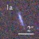
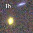
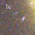
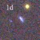
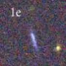
MODEL

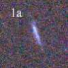
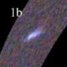
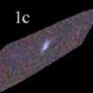
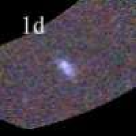
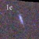
Figure 13: Image system 1: The offsets between the observed and predicted image positions represent the quality of the models. The relatively large offset present in multiple image 1b can result from the nearby cluster galaxy.

RX J1347
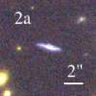
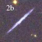
MODEL

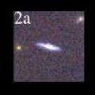
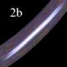
Figure 14: Image system 2:

RX J1347

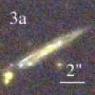
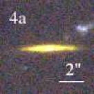
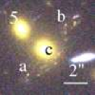
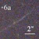
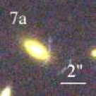
Figure 15: Image systems 3-7:

RX J1347

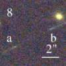
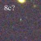
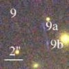
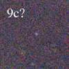
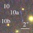
Figure 16: Image systems 8, 9 and 10:

RX J1347

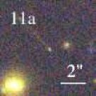
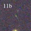
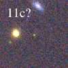
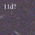
Figure 17: Image system 11:

RX J1347

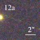
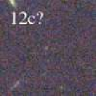
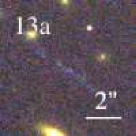
Figure 18: Image systems 12 and 13:

References

- Allen et al. (2002) Allen, S. W., Schmidt, R. W., & Fabian, A. C. 2002, MNRAS, 335, 256
- Bolzonella et al. (2000) Bolzonella, M., Miralles, J.-M., & Pelló, R. 2000, A&A, 363, 476
- Bookstein (1989) Bookstein, F. L. 1989, IEEE Trans. Pattern Anal. Mach. Intell., 11, 567
- Bradač et al. (2005) Bradač, M., Erben, T., Schneider, P., et al. 2005, A&A, 437, 49
- Brainerd et al. (1996) Brainerd, T. G., Blandford, R. D., & Smail, I. 1996, ApJ, 466, 623
- Bruzual & Charlot (2003) Bruzual, G. & Charlot, S. 2003, MNRAS, 344, 1000
- Cohen & Kneib (2002) Cohen, J. G. & Kneib, J.-P. 2002, ApJ, 573, 524
- Fischer & Tyson (1997) Fischer, P. & Tyson, J. A. 1997, AJ, 114, 14
- Fritz et al. (2005) Fritz, A., Ziegler, B. L., Bower, R. G., Smail, I., & Davies, R. L. 2005, MNRAS, 358, 233
- Gitti et al. (2007) Gitti, M., Piffaretti, R., & Schindler, S. 2007, 472, 383
- Gitti & Schindler (2004) Gitti, M. & Schindler, S. 2004, A&A, 427, L9
- Golse & Kneib (2002) Golse, G. & Kneib, J.-P. 2002, A&A, 390, 821
- Halkola et al. (2006) Halkola, A., Seitz, S., & Pannella, M. 2006, MNRAS, 372, 1425
- Halkola et al. (2007) Halkola, A., Seitz, S., & Pannella, M. 2007, ApJ, 656, 739
- Jullo et al. (2007) Jullo, E., Kneib, J.-P., Limousin, M., et al. 2007, ArXiv e-prints, 706
- King (2007) King, L. J. 2007, MNRAS, 956
- Kling et al. (2005) Kling, T. P., Dell’Antonio, I., Wittman, D., & Tyson, J. A. 2005, ApJ, 625, 643
- Koekemoer et al. (2002) Koekemoer, A. M., Fruchter, A. S., Hook, R. N., & Hack, W. 2002, in : The 2002 HST Calibration Workshop : Hubble after the Installation of the ACS and the NICMOS Cooling System., ed. S. Arribas, A. Koekemoer, & B. Whitmore, 337
- Komatsu et al. (2001) Komatsu, E., Matsuo, H., Kitayama, T., et al. 2001, PASJ, 53, 57
- Limousin et al. (2007a) Limousin, M., Kneib, J. P., Bardeau, S., et al. 2007a, A&A, 461, 881
- Limousin et al. (2007b) Limousin, M., Sommer-Larsen, J., Natarajan, P., & Milvang-Jensen, B. 2007b, ArXiv e-prints, 706
- Meneghetti et al. (2007) Meneghetti, M., Argazzi, R., Pace, F., et al. 2007, A&A, 461, 25
- Merritt (1983) Merritt, D. 1983, ApJ, 264, 24
- Natarajan et al. (2002) Natarajan, P., Kneib, J.-P., & Smail, I. 2002, ApJ, 580, L11
- Navarro et al. (1997) Navarro, J. F., Frenk, C. S., & White, S. D. M. 1997, ApJ, 490, 493
- Pointecouteau et al. (1999) Pointecouteau, E., Giard, M., Benoit, A., et al. 1999, ApJ, 519, L115
- Pointecouteau et al. (2001) Pointecouteau, E., Giard, M., Benoit, A., et al. 2001, ApJ, 552, 42
- Ravindranath & Ho (2002) Ravindranath, S. & Ho, L. C. 2002, ApJ, 577, 133
- Sahu et al. (1998) Sahu, K. C., Shaw, R. A., Kaiser, M. E., et al. 1998, ApJ, 492, L125
- Schindler et al. (1995) Schindler, S., Guzzo, L., Ebeling, H., et al. 1995, A&A, 299, L9
- Schindler et al. (1997) Schindler, S., Hattori, M., Neumann, D. M., & Boehringer, H. 1997, A&A, 317, 646
- Schlegel et al. (1998) Schlegel, D. J., Finkbeiner, D. P., & Davis, M. 1998, ApJ, 500, 525
- Tu et al. (2007) Tu, H., Limousin, M., Fort, B., et al. 2007, ArXiv e-prints, 0710.2246
- Ziegler et al. (2001) Ziegler, B. L., Bower, R. G., Smail, I., Davies, R. L., & Lee, D. 2001, MNRAS, 325, 1571