Magneto-spin Hall conductivity of a two-dimensional electron gas

Abstract

It is shown that the interplay of long-range disorder and in-plane magnetic field gives rise to an out-of-plane spin polarization and a finite spin Hall conductivity of the two-dimensional electron gas in the presence of Rashba spin-orbit coupling. A key aspect is provided by the electric-field induced in-plane spin polarization. Our results are obtained first in the clean limit where the spin-orbit splitting is much larger than the disorder broadening of the energy levels via the diagrammatic evaluation of the Kubo-formula. Then the results are shown to hold in the full range of the disorder parameter $\alpha p_{F}\tau$ by means of the quasiclassical Green function technique.

It is well established that the peculiar linear-in-momentum dependence of the Rashba (and of Dresselhaus) spin-orbit coupling leads in a two-dimensional electron gas (2DEG) to the vanishing of the spin Hall conductivityinoue2004 ; mishchenko2004 ; raimondi2005 ; khaetskii2006 . This can be directly recognized by considering the continuity-like equation for the in-plane spin polarization, where the spin-nonconserving terms can be written as the spin current associated to the out-of-plane spin polarization and to the spin Hall effectrashba2004 ; dimitrova2005 ; chalaev2005 . In this paper, we show that the interplay of an in-plane magnetic field, $\mathbf{\mathcal{B}}$, taken parallel to the electric field, $\mathbf{\mathcal{E}}$, (say along the $\hat{\mathbf{e}}_{x}$ axis) and long-range disorder changes this behavior providing then a potential handle on the spin Hall effect. In particular, we show that while the out-of-plane spin polarization is linear in the magnetic field, the spin Hall conductivity is quadratic. Our analysis is valid in the standard good metallic regime $\epsilon_{F}\tau/\hbar\gg 1$ with spin-orbit effects taken into account to first order in $\alpha/v_{F}$. Here $\alpha$ and $\tau$ are the spin-orbit coupling and the elastic quasiparticle lifetime due to impurity scattering, respectively, while $v_{F}$, $p_{F}$ and $\epsilon_{F}=v_{F}p_{F}/2$ are the parameters of the 2DEG in the absence of spin-orbit coupling.

Our proposal of a magnetic field-induced spin Hall effect differs from related previous suggestions both for the analytical treatment of itlin2006 and for the microscopic mechanism responsible of the effectengel2007 . The difference of our proposal with respect to Ref.engel2007 is closely related to the electric field-induced in-plane spin polarization, which for short-range disorder scattering is given by edelstein1990

$$s_{y}=-N_{0}\alpha|e|\mathcal{E}_{x}\tau.$$ (1)

In Eq.(1) $N_{0}=m/(2\pi)$ is the free density of states of the 2DEG in the absence of spin-orbit interaction. Contrary to what one could expect, the generalization of Eq.(1) for long-range disorder, as we will show later, is not the replacement of the elastic quasiparticle lifetime $\tau$ with the transport time, $\tau_{tr}$, as it has been assumed in Ref.[engel2007, ]. We find then that long-range disorder leads to a non-trivial modification of the effective Bloch equations and eventually yields out-of-plane spin polarization and spin Hall effect. In contrast to Ref.[engel2007, ] we do not have to assume a non-parabolicity of the energy bands or an energy dependence of the scattering probability.

Our analysis is carried out in two steps. In the first step, we calculate the out-of-plane spin polarization using the diagrammatic approach of Ref.[raimondi2005, ], valid in the clean limit when the spin-orbit splitting is much larger than the disorder-induced broadening, $2\alpha p_{F}\gg\tau^{-1}$. In order to make contact with the analysis of Ref.[engel2007, ] performed in the opposite dirty limit ($\alpha p_{F}\ll\tau^{-1}$), we present, in the second step, a derivation based on the Eilenberger equation for the quasiclassical Green function in the presence of spin-orbit couplingraimondi2006 . The advantage of so doing is that the analysis is valid for an arbitrary value of the parameter $2\alpha p_{F}\tau$ and also allows to determine the effective Bloch equations for the spin density.

The Hamiltonian of a 2DEG perpendicular to the $\hat{\mathbf{e}}_{z}$-axis reads

$$H=\frac{{\bf p}^{2}}{2m}+\mathbf{b}(\mathbf{p})\cdot\boldsymbol{\sigma}+V(\mathbf{x})$$ (2)

where ${\bf b}({\bf p})=\alpha\mathbf{p}\times\hat{\mathbf{e}}_{z}-\omega_{s}\hat{\mathbf{e}}_{x}$ is the effective magnetic field including both the Rashba spin-orbit coupling and the external magnetic field. In Eq.(2), $V(\mathbf{x})$ describes the potential scattering from the impurities and, according to the established procedure in the literature, will be taken as a random variable.

The possibility of a non-vanishing spin Hall conductivity in the presence of an in-plane field may be appreciated by considering the equation of motion for the $\hat{\mathbf{e}}_{y}$-axis (in-plane) spin polarization, which yields

$$\frac{\partial s_{y}}{\partial t}+\frac{\partial}{\partial\mathbf{x}}\cdot\mathbf{j}^{y}_{s}=-2m\alpha j_{s,y}^{z}+2\omega_{s}s_{z},$$ (3)

where $j_{s,\gamma}^{i}$ is the $\hat{\mathbf{e}}_{\gamma}$-axis component of the spin current that is polarized along the $\hat{\mathbf{e}}_{i}$-axis. Under stationary and uniform conditions, the above equation implies, in the absence of the magnetic field, a vanishing spin current and hence a vanishing spin Hall conductivity, with the latter defined by $j^{z}_{s,y}=\sigma_{s,H}\mathcal{E}_{x}$. In the presence of an in-plane magnetic field one may have a bulk spin Hall current determined by

$$j^{z}_{s,y}=\frac{\omega_{s}}{\alpha m}s_{z}.$$ (4)

In the following we evaluate $s_{z}$ to first order in the magnetic field which implies that of $j^{z}_{s,y}$ to second order.

As anticipated, we begin by sketching the calculation performed with the diagrammatic approach. To linear order in the electric field, the Kubo formula for the zero-temperature expression of the out-of-plane spin polarization reads

$$s_{z}=-\frac{1}{2\pi}\sum_{\mathbf{p}}\mathrm{Tr}_{\sigma}\left[\overline{s_{z}G^{R}(\mathbf{p})j_{c}^{x}G^{A}(\mathbf{p})}\right]|e|\mathcal{E}_{x},$$ (5)

where the Green functions can be obtained from Eq.(2), the vertices are $s_{z}=(1/2)\sigma_{z}$, $j_{c}^{x}=(p_{x}/m)\sigma_{0}-\alpha\sigma_{y}$, and the trace is over the associated spin indices. In Eq.(5), the bar indicates the average over the impurity potential, which, at the level of the self-consistent Born approximation, yields the self-energy

$$\Sigma^{R,A}(\mathbf{p})=\sum_{\mathbf{p}^{\prime}}|V({\mathbf{p}-\mathbf{p}^{\prime}})|^{2}G^{R,A}(\mathbf{p}^{\prime}),$$ (6)

$|V(\mathbf{q})|^{2}$ being the Fourier transform of $\overline{V(\mathbf{x})V(\mathbf{x}^{\prime})}$. In order to consider the effect of long-range disorder, we expand the above scattering probability as

$$|V|^{2}=V_{0}+2V_{1}\cos(\varphi-\varphi^{\prime})+2V_{2}\cos(2\varphi-2\varphi^{\prime})+\cdots,$$ (7)

where $\varphi-\varphi^{\prime}$ is the angle between the two momenta $\mathbf{p}$ and $\mathbf{p}^{\prime}$. The harmonics, $V_{0}$, $V_{1}$, $V_{2}$ are functions of $|\mathbf{p}|$ and $|\mathbf{p}^{\prime}|$. In the following we will ignore this dependencenotefour and take both momenta at $p_{F}$. To first order in the magnetic field the diagrams to be evaluated are shown in Fig.1. Notice that all the vertices and propagators appearing in the diagrams must be evaluated at zero magnetic field.

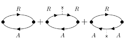
Figure 1: Diagrams to be evaluated in zeroth and first order in the magnetic field. The dashed line ending with a cross indicates the magnetic field insertion. Under impurity average the (spin density and charge current) vertices are dressed by the standard ladder resummation.

It is then convenient, following Ref.[raimondi2005, ], to use the disorder-free Hamiltonian eigenstates

$$|\mathbf{p}\pm\rangle=\frac{1}{\sqrt{2}}\left(\pm\mathrm{i}\exp(-\mathrm{i}\varphi)|\mathbf{p}\uparrow\rangle+|\mathbf{p}\downarrow\rangle\right)$$ (8)

corresponding to the eigenvalues $E_{\pm}=p^{2}/2m\pm\alpha p$ with $\tan(\varphi)=p_{y}/p_{x}$. In terms of the transformation matrix, $U$, defined by Eq.(8), the Pauli matrices transform as

$$\begin{array}[]{ccc}U\sigma_{x}U^{{\dagger}}&=&\hat{p}_{y}\sigma_{z}+\hat{p}_{x}\sigma_{y}\\ U\sigma_{y}U^{{\dagger}}&=&-\hat{p}_{x}\sigma_{z}+\hat{p}_{y}\sigma_{y}\\ U\sigma_{z}U^{{\dagger}}&=&-\sigma_{x}\end{array},\begin{array}[]{ccc}\hat{p}_{x}&\equiv&\cos(\varphi)\\ \hat{p}_{y}&\equiv&\sin(\varphi)\end{array}.$$ (9)

As a consequence the spin density vertex, the magnetic field insertion and the charge current vertex become

$$Us_{z}U^{{\dagger}} = -\frac{1}{2}\sigma_{x},$$ (10)

$$U(-\omega_{s}\sigma_{x})U^{{\dagger}} = -\omega_{s}(\hat{p}_{y}\sigma_{z}+\hat{p}_{x}\sigma_{y}),$$ (11)

$$Uj_{c}^{x}U^{\dagger} = \left(\frac{p}{m}\sigma_{0}+\alpha\sigma_{z}\right)\hat{p}_{x}-\sigma_{y}\hat{p}_{y}.$$ (12)

Upon impurity averaging the spin and charge vertices get renormalized. In terms of the renormalized quantities, Eq.(5) becomes to first order in the Zeeman field

$$s_{z}=-\mathrm{i}\omega_{s}\frac{|e|\mathcal{E}_{x}}{4\pi}\sum_{\mathbf{p}}^{\mu=\pm}\hat{p}_{x}\mu(\Gamma_{\mu\bar{\mu}}G^{R}_{\bar{\mu}}-\Gamma_{\bar{\mu}\mu}G^{A}_{\bar{\mu}})G^{R}_{\mu}G^{A}_{\mu}J_{c,\mu\mu},$$ (13)

where the first (second) term in the brakets refers to the magnetic field insertion in the top (bottom) Green function line and $\mu=\pm$ labels the eigenstates. The quantities $\Gamma_{\mu\mu^{\prime}}$ and $J_{c,\mu\mu^{\prime}}$ are the dressed vertices corresponding to $s_{z}$ and $j_{c}^{x}$, respectively, and the Green functions are evaluated via the self-energy given in Eq.(6). Apart from the spin vertex $\Gamma_{\mu\mu^{\prime}}$, all the other quantities have been evaluated in Ref.[raimondi2005, ], where it has been shown that the off-diagonal matrix element $J_{c,\mu\bar{\mu}}$ vanishes and the self-energy is diagonal in the eigenstate basis with

$$\Sigma^{R(A)}_{\pm}=\frac{-(+)\mathrm{i}}{2\tau_{\pm}},\ \tau_{\pm}=\tau\left(1\pm\frac{V_{1}}{V_{0}}\frac{\alpha}{v_{F}}\right),\frac{1}{\tau}=2\pi N_{0}V_{0}.$$ (14)

The spin vertex obeys the equation

$$\Gamma_{\mu\bar{\mu}}=1+\sum_{\mathbf{p^{\prime}}}^{\nu=\pm\mu}\Gamma_{\nu\bar{\nu}}G^{R}_{\bar{\nu}}G^{A}_{\nu}|V|^{2}\frac{1+\mu\nu\cos(\varphi-\varphi^{\prime})}{2},$$ (15)

which yields

$$\Gamma_{\mu\bar{\mu}}=1+\frac{\mathrm{i}\mu}{2\alpha p_{F}\tau}\frac{V_{1}}{V_{0}}.$$ (16)

By using $G^{R}_{\mu}G^{A}_{\mu}=\mathrm{i}\tau_{\mu}(G^{R}_{\mu}-G^{A}_{\mu})$, integrating over the energy, $\xi=p^{2}/2m-\mu$, and keeping terms up to order $\alpha/v_{F}$, Eq.(13) becomes

$$s_{z}=-|e|\mathcal{E}_{x}\frac{\omega_{s}}{8\alpha^{2}\tau}\left(1-\frac{V_{1}}{V_{0}}\right)\sum_{\mu=\pm}\mu\frac{N_{\mu}J_{\mu}\tau_{\mu}}{p_{\mu}^{2}},$$ (17)

where $N_{\pm}=N_{0}(1\mp\alpha/v_{F})$, $p_{\pm}=p_{F}(1\mp\alpha/v_{F})$ are the density of states and the Fermi momentum of the two spin subbands and $J_{\pm\pm}(p_{\pm})=J_{\pm}\hat{p}_{x}$ are the Fermi-surface expressions of the charge vertices. Finally, borrowing from Ref.[raimondi2005, ] the expression for the vertices

$$J_{\pm}=v_{F}\left(\frac{V_{0}}{V_{0}-V_{1}}\mp\frac{\alpha}{v_{F}}\frac{V_{0}+V_{2}}{V_{0}-V_{2}}\right),$$ (18)

one gets the out-of-plane spin polarization

$$s_{z}=-\frac{1}{2}|e|\mathcal{E}_{x}\frac{\omega_{s}}{\alpha p_{F}}\frac{N_{0}}{p_{F}}\frac{V_{1}-V_{2}}{V_{0}-V_{2}}$$ (19)

and, via Eq.(4), the spin Hall conductivity

$$\sigma_{sH}=-\frac{|e|}{4\pi}\left(\frac{\omega_{s}}{\alpha p_{F}}\right)^{2}\frac{V_{1}-V_{2}}{V_{0}-V_{2}}.$$ (20)

Remarkably the above central result shows that the sign of the spin Hall conductivity depends on the relative strength of the harmonics of the scattering probability. This may explain the sign change in the numerical evaluation of Ref.lin2006 . On the other hand, Eq.(19) is inconsistent with Ref.engel2007 , where for the disorder model of Eq.(7) one would expect a vanishing out-of-plane polarization.

Recall that we derived Eqs.(19) and (20) in the clean limit. We now rederive the above results by means of the kinetic equations approach of Ref.[raimondi2006, ] and find that Eqs.(19) and (20) are valid for all values of the disorder parameter $\alpha p_{F}\tau$. Furthermore we will derive the effective Bloch equations in the dirty limit. We start with the Eilenberger equation

$$\partial_{t}\check{g} = -\frac{1}{2}\sum_{\mu=\pm}\left\{\frac{\bf p_{\mu}}{m}\right.+\left.\frac{\partial}{\partial\bf p}({\bf b}_{\mu}\cdot{\boldsymbol{\sigma}}),\frac{\partial}{\partial{\bf x}}\check{g}_{\mu}\right\}$$ (21)

$$- {\rm i}\sum_{\mu=\pm}[{\bf b}_{\mu}\cdot{\boldsymbol{\sigma}},\check{g}_{\mu}]-{\rm i}\left[\check{\Sigma},\check{g}\right]$$

for the quasiclassical Green function ($\check{g}\equiv\check{g}_{t_{1}t_{2}}(\mathbf{\hat{p}};\mathbf{x})$)

$$\check{g}=\frac{\rm i}{\pi}\int{\rm d}\xi\,\check{G}_{t_{1}t_{2}}(\mathbf{p},\mathbf{x}),\ \check{G}=\left(\begin{array}[]{cc}G^{R}&G\\ 0&G^{A}\end{array}\right)$$ (22)

where $\check{G}_{t_{1}t_{2}}(\mathbf{p},\mathbf{x})$ is the Wigner representation of the Green function, which has both matrix structure in the Keldysh (denoted by the check symbol) and spin spaces. $[,]$ and $\{,\}$ indicate commutator and anticommutator. As for the diagrammatic approach, the index $\mu=\pm$ labels the two spin subbands ($\mathbf{b}_{\pm}=\mathbf{b}(\mathbf{p}_{\pm})$). In integrations like in Eq.(22) the corresponding poles in the Green functions yield the two-component decomposition of the quasiclassical Green function

$${\check{g}}_{\pm}=\frac{1}{2}\Big{\{}\frac{1}{2}(1\pm{\hat{\bf b}}_{0}\cdot{\boldsymbol{\sigma}}),{\check{g}}\Big{\}}.$$ (23)

The ”0” subscript denotes evaluation at the Fermi surface in the absence of spin-orbit coupling. In the following we are going to use Eq.(21) to first order in the parameter $|{\bf b}_{0}|/\epsilon_{F}$. The connection to the physical observables is made by integrating over the energy $\epsilon$, which is the Fourier conjugated variable of the time difference $t_{1}-t_{2}$. For instance, the out-of-plane spin density is given by the angular average of the Keldysh componentnotethree

$$s_{z}=s_{z}^{eq}-\frac{N_{0}}{8}\int\mathrm{d}\epsilon\langle\mathrm{Tr}(\sigma_{z}g)\rangle,\ \langle...\rangle\equiv\int_{0}^{2\pi}\frac{\mathrm{d}\phi}{2\pi}...\ .$$ (24)

In order to solve, to linear order in the electric field, the Keldysh component of the Eilenberger equation (21), we use the minimal substitution $\partial_{\mathbf{x}}g\rightarrow-|e|\mathcal{E}_{x}{\hat{\bf e}}_{x}\partial_{\epsilon}g_{eq}$ where $g_{eq}=\tanh(\epsilon/2T)(g^{R}_{eq}-g^{A}_{eq})$ with $g^{R}_{eq}=-g^{A}_{eq}=1-\partial_{\xi}\mathbf{b}_{0}\cdot{\boldsymbol{\sigma}}$ is the equilibrium quasiclassical Green function. As in the diagrammatic treatment previously developed, we find it convenient to transform the equations to the eigenstate basis via Eq.(9). After expressing the quasiclassical Green function as a four-dimensional column vector

$$\tilde{g}=UgU^{\dagger}=\tilde{g_{0}}\sigma_{0}+\mathbf{\tilde{g}}\cdot{\boldsymbol{\sigma}}\rightarrow\left(\begin{array}[]{ cccc}\tilde{g_{0}}&\tilde{g_{3}}&\tilde{g_{1}}&\tilde{g_{2}}\end{array}\right)^{t},$$ (25)

the Eilenberger equation (21) can be then written as a linear system of four equations for the components of $\tilde{g}$

$$\partial_{t}\tilde{g}=-\frac{1}{\tau}(M_{0}+M_{1})\tilde{g}+\frac{1}{\tau}(1+N)\langle K\tilde{g}\rangle+S_{0}+S_{1},$$ (26)

where,

$$N = -\frac{\alpha}{v_{F}}\left(\begin{array}[]{cccc}0&1&0&0\\ 1&0&0&0\\ 0&0&0&0\\ 0&0&0&0\end{array}\right)$$ (31)

$$M_{0} = 1+\frac{V_{1}}{V_{0}}N+2\alpha p_{F}\tau\left(\begin{array}[]{cccc}0&0&0&0\\ 0&0&0&0\\ 0&0&0&1\\ 0&0&-1&0\end{array}\right)$$ (36)

$$M_{1} = 2\omega_{s}\tau\left(\begin{array}[]{cccc}0&0&0&0\\ 0&0&-\hat{p}_{x}&0\\ \frac{\alpha}{v_{F}}\hat{p}_{x}&\hat{p}_{x}&0&-\hat{p}_{y}\\ 0&0&\hat{p}_{y}&0\end{array}\right).$$ (41)

In Eq.(26), $\langle...\rangle$ denotes angle integration over $\varphi^{\prime}$ with the scattering kernel that can be expandend into angular harmonics as

$$K(\varphi-\varphi^{\prime})=K^{(0)}+\cos(\varphi-\varphi^{\prime})K^{(a)}+\sin(\varphi-\varphi^{\prime})K^{(b)}+\cdots$$ (42)

each coefficient being itself a matrix

$$K^{(0)}=\left(\begin{array}[]{cccc}1&0&0&0\\ 0&\frac{V_{1}}{V_{0}}&0&0\\ 0&0&1&0\\ 0&0&0&\frac{V_{1}}{V_{0}}\end{array}\right),K^{(b)}=\frac{V_{0}-V_{2}}{V_{0}}\left(\begin{array}[]{cccc}0&0&0&0\\ 0&0&0&1\\ 0&0&0&0\\ 0&-1&0&0\end{array}\right)$$

and

$$K^{(a)}=\frac{1}{V_{0}}\left(\begin{array}[]{cccc}2V_{1}&0&0&0\\ 0&V_{0}+V_{2}&0&0\\ 0&0&2V_{1}&0\\ 0&0&0&V_{0}+V_{2}\end{array}\right).$$

Finally the source electric-field dependent terms are

$$S_{0}=E\left(\begin{array}[]{c}\hat{p}_{x}\\ -\frac{\alpha}{v_{F}}\hat{p}_{x}\\ 0\\ -\frac{\alpha}{v_{F}}\hat{p}_{y}\end{array}\right),S_{1}=\frac{\omega_{s}}{v_{F}p_{F}}E\left(\begin{array}[]{c}0\\ \hat{p}_{x}\hat{p}_{y}\\ 0\\ \hat{p}_{x}^{2}\end{array}\right),$$

with $E=|e|\mathcal{E}_{x}v_{F}\partial_{\epsilon}(2\tanh(\epsilon/2T))$. Notice that, consistently with the accuracy we are working, one may use for the charge density component the solution obtained in the absence of both spin-orbit coupling and magnetic field

$$j_{c,x}\sim\langle\hat{p}_{x}\tilde{g}_{0}^{(0)}\rangle=\frac{1}{2}\frac{V_{0}}{V_{0}-V_{1}}\tau E,$$ (43)

where the characteristic transport time renormalization $\tau_{tr}=\tau V_{0}/(V_{0}-V_{1})$ appears. We seek now a stationary solution of Eq.(26) which is evaluated in first order in the magnetic field $\tilde{g}=\tilde{g}^{(0)}+\tilde{g}^{(1)}+\dots$. We then get

$$\langle\tilde{g}^{(1)}\rangle=(M_{0}-K^{(0)})^{-1}(\tau\langle S_{1}\rangle-\langle M_{1}\tilde{g}^{(0)}\rangle).$$ (44)

According to the transformation of Eq.(10), the out-of-plane spin polarization is related to

$$s_{z}\sim\langle\tilde{g}^{(1)}_{1}\rangle=-\frac{\omega_{s}}{2\alpha p_{F}}\left(\frac{1}{v_{F}p_{F}}E+\frac{1}{\alpha p_{F}\tau}\frac{V_{0}-V_{1}}{V_{0}}\langle\hat{p}_{x}\tilde{g}^{(0)}_{3}\rangle\right),$$ (45)

which is expressed in terms of $\langle\hat{p}_{x}\tilde{g}_{3}\rangle$ evaluated at zero magnetic field. This latter quantity is nothing but the in-plane spin polarization (cf. the second line of Eq.(9)). By multiplying the second component of the system Eq.(26) by $\hat{p}_{x}$ and performing the angle average, one obtains the generalization, for long-range disorder, of the Edelstein resultedelstein1990

$$s_{y}\sim\langle\hat{p}_{x}\tilde{g}^{(0)}_{3}\rangle=-\frac{\alpha}{v_{F}}\frac{V_{0}}{V_{0}-V_{2}}\tau E.$$ (46)

Finally, by using Eqs.(45,46) into Eq.(24) one recovers the result (19) of the diagrammatic approach, which is now manifestly valid for any strength of the disorder. To understand the meaning of Eq.(46), it is useful to recall the origin of the in-plane polarizationedelstein1990 : In the presence of an electric field the Fermi surface is shifted by $\delta p_{x}\sim|e|\mathcal{E}_{x}\tau$. As a result the total spin of the electrons neither in the plus nor in the minus band adds up to zero. Although the contributions of both bands tend to cancel, a finite spin polarization remains due to the $\alpha/v_{F}$ corrections in the density of states. For long-range disorder, the Fermi surface shift is proportional to the transport time $\tau_{tr}$, so one might expect the transport time also in the in-plane spin polarization. However due to the $\alpha/v_{F}$ corrections each band has its own effective transport time, $\tau_{tr,\pm}\equiv J_{\pm}\tau_{\pm}/v_{F}$ and the explicit result reads ($s_{0}=\alpha N_{0}|e|\mathcal{E}_{x}\tau$)

$$s_{y}=\frac{v_{F}}{4}(N_{+}\tau_{tr,+}-N_{-}\tau_{tr,-})|e|\mathcal{E}_{x}=-\frac{V_{0}}{V_{0}-V_{2}}s_{0}.$$ (47)

At last we study the combined effect of magnetic and electric field in the diffusive regime, $\omega_{s}\tau,\alpha p_{F}\tau\ll 1$. The effective Bloch equations for the spin density are

$$\partial_{t}s_{x} = -\tau_{s}^{-1}(s_{x}-s_{x}^{eq})$$ (48)

$$\partial_{t}s_{y} = -\tau_{s}^{-1}\left[s_{y}+s_{0}V_{0}/(V_{0}-V_{2})^{-1}\right]+2\omega_{s}s_{z}$$ (49)

$$\partial_{t}s_{z} = -2\tau_{s}^{-1}s_{z}-2\omega_{s}\left[s_{y}+s_{0}\tau_{tr}/\tau\right],$$ (50)

where $\tau_{s}^{-1}=2(\alpha p_{F})^{2}\tau_{tr}$ and $s_{x}^{eq}=N_{0}\omega_{s}$. Eqs.(48) and (50) agree with what was found in Ref.engel2007 , the only difference is in the term proportional to the electric field (i.e. $s_{0}$) in Eq.(49). The stationary spin polarization as a function of magnetic field is now determined as

$$s_{y} = -\frac{V_{0}\,s_{0}}{V_{0}-V_{2}}\frac{1+2\omega_{s}^{2}\tau_{s}^{2}(V_{0}-V_{2})(V_{0}-V_{1})^{-1}}{1+2\omega_{s}^{2}\tau_{s}^{2}}$$ (51)

$$s_{z} = -\frac{V_{0}\,s_{0}}{V_{0}-V_{2}}\frac{V_{1}-V_{2}}{V_{0}-V_{1}}\frac{\omega_{s}\tau_{s}}{1+2\omega_{s}^{2}\tau_{s}^{2}}$$ (52)

showing an out-out-plane contribution as observed experimentally in Ref.kato2004 .

In conclusion, we have shown that the combined effect of an in-plane magnetic field, long-range disorder and spin-orbit coupling gives rise to an out-of-plane spin polarization and finite spin Hall conductivity, whose value does not depend on the concentration of defects as long as the 2DEG is in the metallic regime. To obtain the correct value of the electric-field induced in-plane spin polarization it is essential to take into account the different transport times in the two spin-orbit splitted bands.

We acknowledge financial support by the Deutsche Forschungsgemeinschaft through SFB 484 and SPP 1285 and by CNISM under Progetti Innesco 2006. R.R. thanks the kind hospitality of the ICTS, Jacobs University, Bremen, where this work was initiated.

References

• (1) J. I. Inoue, G. E. W. Bauer, and L. W. Molenkamp, Phys. Rev. B 70, 041303(R) (2004).
• (2) E. G. Mishchenko, A. V. Shytov, and B. I. Halperin, Phys. Rev. Lett. 93, 226602 (2004).
• (3) R. Raimondi and P. Schwab, Phys. Rev. B 71, 033311 (2005).
• (4) A. Khaetskii, Phys. Rev. Lett. 96, 056602 (2006).
• (5) E. I. Rashba, Phys. Rev. B 70, 201309(R) (2004).
• (6) O. V. Dimitrova, Phys. Rev. B 71, 245327 (2005).
• (7) O. Chalaev and D. Loss, Phys. Rev. B 71, 245318 (2005).
• (8) Q. Lin, S. Y. Liu, and X. L. Lei, Appl. Phys. Lett. 88, 122105 (2006).
• (9) H. A. Engel, E. I. Rashba, and B. Halperin, Phys. Rev. Lett. 98, 036602 (2007).
• (10) V. M. Edelstein, Solid State Commun. 73, 233 (1990).
• (11) R. Raimondi, C. Gorini, P. Schwab, and M. Dzierzawa, Phys. Rev. B 74, 035340 (2006).
• (12) Hence, we neglect the effects described, in Ref.engel2007 , by the scattering kernel $\widetilde{K}$.
• (13) Within the quasiclassical formalism, $g$ describes the dynamic part only to which add the equilibrium part.
• (14) Y. K. Kato, R. C. Myers, A. C. Gossard, and D. D. Awschalom, Phys. Rev. Lett. 93, 176601 (2004).