The Geometrical Effects on Electronic Spectrum and Persistent Currents in Mesoscopic Polygon

Abstract

In this paper, a new mesoscopic polygon which possesses smooth transition at its corners is proposed. Because of the particularity of structure, this kind of mesoscopic polygon can also be a geometrical supperlattice. The geometrical effects on the electron states and persistent current are investigated comprehensively in the presence of magnetic flux. We find that the particular geometric structure of the polygon induces an effective periodic potential which results in gaps in the energy spectrum. The changes of gaps show the consistency with the geometrical twoness of this new polygon. This electronic structure and the corresponding physical properties are found to be periodic with period $\phi_{0}$ in the magnetic flux $\phi$ and can be controlled by the geometric method. We also consider the Rahsba spin-orbit interaction which make the energy levels splitting newly to double and leads to an additional small zigzag in one period of the persistent current. These new phenomena may be useful for the applications in quantum device design in the future.

The rapid developments of advanced growth techniques make it possible to fabricate reduced-dimensional quantum systems with complex geometries which attract much attentions in recent years^[1-4]. The fabrication of essentially arbitrary geometries could lead to dramatic control of the electronic properties of solids by means of geometries. For example, ringlike structures of semiconductor have become the subject of extensive theoretical and experimental studies because of their unique topologies and potential applications in the spintronics nanodevices^[5], which utilize the spin rather than the charge of an electron. A prime candidate for spin manipulation is the Rashba spin-orbit interaction (SOI)^[6], which stems from the absence of structure inversion symmetry. For ring structures, the energy spectrum and the interference effects due to the SOI have been well investigated^[7] and for square loops it has been shown^[8] that interference due to Rashba SOI can lead to electron localization. Recently, the spin-interference of ballistic electrons traveling along any regular polygon is also studied^[9,10] and shows a dependence on the sidelength and alignment of the polygon as well as on the SOI constant.

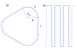
Figure 1: (a) Sketch of a mesoscopic polygon ($N=3$) in the x-y plane. (b) The corresponding periodic structures of the geometrical potential.

Besides the quantum rings, many of the fabrication structures exhibit curvature on the nanoscale, such as nanotubes^[2], nanotori^[3], the spiral inductors^[11], quantum snakes, and so on. These curvilinear structures have been the focus on investigation of new physical features that appear due to the curvature.^[12] When the electron is strongly confined to a low dimensional curvilinear system with smooth geometry, the interplay between geometry and quantum physics results in an effective geometric potential whose magnitude depends on the local curvature.^[13] This implies that the quantum behaviors of the electron can be controlled by altering the local geometric curvature. Such an effective geometric potential has successfully applied, for example, to the band-structure calculation of real systems^[14], to the determination of electron states in curvilinear quantum wires^[15] and to the impact of curvature on electron transportation in different curved systems^[16,17,18]. Furthermore, experiment of localized states of high oxidized porous silicon^[19] indicates that the curvature potential plays important roles in the electronic behaviors. However, the studies on electronics and spintronics of the ringlike structure, square loop and regular polygon did not deal with the curvature potential. What are the effects of the curvature potential is significant to investigate in curved mesoscopic systems.

In this paper, we focus on the polygonal structures of the semiconductor^[20]. Considering that the edges of the nano-polygon always have the width, we establish an extended one-dimensional model of mesoscopic regular polygon with smooth transition at its corners. We point out that this mesoscopic polygon takes more further freedom on controlling the electron behaviors. The curvature effects are taken into account through introducing the geometrical potential. Because magnetic field effects prove important to the interference phenomena, the electronic spectrum and persistent currents of electrons in the mesoscopic polygon are theoretically investigated in the presence of magnetic flux. The Rashba SOI is also considered.

Geometrically, our mesoscopic polygon consists of $N$ straight line segments and $N$ arc segments forming a periodic structure with the $C_{N}$ symmetry. As shown in Fig. 1 (a), the circumference is $L=N\left(l_{1}+l_{2}\right)$ where $l_{1}$ is the length of one straight line and $l_{2}=R\theta_{m}=2\pi R/N$ for an arc with the curvature radius $R$ and the arc angle $\theta_{m}$. We can see that this mesoscopic polygon, which trends to a perfect ring for the limit of $l_{1}\rightarrow 0$ and to a regular polygon for the limit of $R\rightarrow 0$, shows a geometrical twoness. The curvature can arise an effective geometric potential with the form $V_{g}=-\hbar^{2}\kappa^{2}/(8m)^{[17]}$, where $\kappa$ is the curvature of the wire. Form Fig. 1 (b), it is obvious that the geometric potentials form a structure of periodic square potential. So the mesoscopic polygon can be regarded as a geometrical supperlattice.

We consider a mesoscopic polygon in the $x-y$ plane subjected to an axial magnetic field $B$ which is oriented through the $z$ axis. For a convenient choice of magnetic vector, the Hamiltonians in the presence of the Rashba SOI^[6] for a conduction electron of the effective mass $m$ are given by^[18]

$$H_{line}=-\frac{\hbar^{2}}{2m}\frac{\partial^{2}}{\partial s^{2}}+i\frac{e\hbar}{c}A_{s}\frac{\partial}{\partial s}+\frac{e^{2}}{2mc^{2}}A_{s}^{2}-i\alpha\sigma_{b}(\frac{\partial}{\partial s}+i\frac{e\hbar}{c}A_{s}),$$ (1)

$$H_{arc}=-\frac{\hbar^{2}}{2m}\frac{\partial^{2}}{\partial s^{2}}+i\frac{e\hbar}{c}A_{s}\frac{\partial}{\partial s}-\frac{\hbar^{2}\kappa^{2}}{8m}+\frac{e^{2}}{2mc^{2}}A_{s}^{2}-i\alpha[\sigma_{b}(\frac{\partial}{\partial s}+i\frac{e\hbar}{c}A_{s})-\frac{1}{2}\sigma_{t}\kappa],$$ (2)

where $A_{s}$ is the component of vector potential ${\bf A}$ along the arclength $s$ direction, $\sigma_{b}={\bf\hat{\sigma}}\cdot$ ${\bf b}$ and $\sigma_{t}={\bf\hat{\sigma}}\cdot$ ${\bf t}$, expressed by the usual Pauli matrices $\hat{\sigma}_{x,y,z}$, are the spin matrices on the normal ${\bf b}$ and tangent ${\bf t}$ direction, respectively. The parameter $\alpha$ is the Rashba strength which represents the average electric field along the $z$ direction and can be controlled by a gate voltage.

Both the wave function in the straight lines $\Psi_{1}$ and the wave function in the arc $\Psi_{2}$ should satisfy the Bloch theorem and two boundary conditions^[21]:

(i) the Bloch theorem reads

$$\Psi_{1,2}(s+l_{1}+l_{2})=e^{iK(l_{1}+l_{2})}\Psi_{1,2}(s),$$ (3)

where $K$ is the wave vector in the reciprocal-space.

(ii) the boundary conditions at $s=0,L$ ($L=N(l_{1}+l_{2})$ is the circumference of mesoscopic polygon) are

$$\Psi_{1}(0)=e^{i2\pi(\phi/\phi_{0})}\Psi_{2}(L),\frac{\partial\Psi_{1}(0)}{\partial s}=\frac{\partial\Psi_{2}(L)}{\partial s},$$ (4)

where $\phi$ is the magnetic flux along the $z$ direction through the area confined by the mesoscopic polygon and $\phi_{0}$ is the magnetic flux quantum. From Eqs. (3) and (4), we get the relationship $KL=2\pi(n+\phi/\phi_{0}),n=0,1,2,...$. It is obviously that Eq. (4) imply that the electronic spectra of mesoscopic polygon are periodic in $\phi$ with period $\phi_{0}$, and so are the other physical properties.

(iii) the boundary conditions at the connecting points $s=m(l_{1}+l_{2})+l_{1},m=0,1,...,N-1$ or$\ s=m(l_{1}+l_{2}),m=1,...,N-1$ are

$$\Psi_{1}(s)=\Psi_{2}(s),\frac{\partial\Psi_{1}(s)}{\partial s}=\frac{\partial\Psi_{2}(s)}{\partial s}.$$ (5)

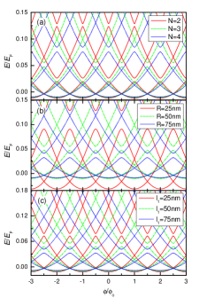
Figure 2: The electron energy levels in the mesoscopic polygon as a function of the magmatic flux $\phi$ in the absence of SOI ($\alpha=0$). The energy spectrum is shown for $N=2$, $3$, $4$ at $R=50$ nm and $l_{1}=$ $50$ nm in (a), for $R=25$ nm, $50$ nm, $70$ nm at $N=3$ and $l_{1}=$ $50$ nm in (b), and for $l_{1}=25$ nm, $50$ nm, $75$ nm at $N=3$ and $R=$ $50$ nm in (c).

When there isn’t Rashba SOI, i. e. $\alpha=0$, using the above conditions we can easily obtain a transcendental equation defining the energy spectrum for unbound states $E>0$

$$\cos(k_{2}l_{2})\cos(k_{1}l_{1})-\sin(k_{2}l_{2})\sin(k_{1}l_{1})\left(\frac{k_{1}^{2}+k_{2}^{2}}{2k_{1}k_{2}}\right)=\cos[\frac{2\pi}{N}(n+\frac{\phi}{\phi_{0}})]$$ (6)

where $k_{1}=\sqrt{2mE/\hbar^{2}}$ is the wave vector for straight lines and $k_{2}=\sqrt{2m(E+V_{g})/\hbar^{2}}$ for arc. While for bounded states $-V_{g}<E<0$

$$\cos(k_{2}l_{2})\cosh(\tilde{k}_{1}l_{1})-\sin(k_{2}l_{2})\sinh(\tilde{k}_{1}l_{1})\left(\frac{\tilde{k}_{1}^{2}-k_{2}^{2}}{2\tilde{k}_{1}k_{2}}\right)=\cos[\frac{2\pi}{N}(n+\frac{\phi}{\phi_{0}})],$$ (7)

here $\tilde{k}_{1}=\sqrt{-2mE/\hbar^{2}}$ and $\phi$ is the magnetic flux through the area confined by the mesoscopic polygon.

For InAs material, the effective electron mass $m=0.023m_{0}$ and the Fermi energy $E_{F}=11.13\times 10^{-3}$ eV. The calculated energy spectra as a function of the magnetic field flux for a different set of $N$, $R$ and $l_{1}$ are given in Fig. 2, respectively. Different from the status in the perfect rings where the energy levels are intersecting parabolas, the gaps are opened at the points of intersection of the parabolas in our mesoscopic polygon. The whole energy levels are periodic curves with a period of $\phi_{0}$. In addition, if the mesoscopic polygon circumference increases through changing the geometrical parameters $N,$ $R$ and $l_{1}$, the energy levels tend to flat and have the negative shifts which are larger at higher energy. It is obvious that there exit the bound states of $E<0$ in the energy spectra. Our results are consistent with the known fact that there is one and only one bound state for $\theta_{m}=2\pi/N\leq\pi$ in such a quadrate trap formed by the geometric potential^[12]. Additionally, one can see that the bound state of the mesoscopic polygon can transform to the unbound state smoothly in the presence of the magnetic flux. So there will be a contribution to the persistent current from the bound state.

When there is Rashba SOI, the transcendental equation defining the energy spectrum for unbound states $E>0$ obtained from the boundary conditions is

$$-2f^{2}\{\cos[\frac{4\pi}{N}(\frac{\phi}{\phi_{0}}+n+\frac{1}{2})]+\cos(2bl_{1})+\cos(2dl_{2})+3\cos(dl_{2})\cos(bl_{1})$$ (8)

$$-4\cos(2\lambda)\sin^{2}(dl_{2})\sin^{2}(bl_{1})-4\sin(\lambda)\sin(2dl_{2})\sin(2bl_{1})\}$$

$$-16f\cos[\frac{2\pi}{N}(\frac{\phi}{\phi_{0}}+n+\frac{1}{2})][\cos(dl_{2})\cos(bl_{1})-\sin(dl_{2})\sin(bl_{1})\sin(\lambda)]$$

$$\times[2f\cos(cl_{2})\cos(al_{1})-(1+f^{2})\sin(cl_{2})\sin(al_{1})]$$

$$-[(1+6f^{2}+f^{4})\cos(2cl_{2})-(1-f^{2})^{2}]\cos(2al_{1})$$

$$+4f(1+f^{2})\sin(2cl_{2})\sin(2al_{1})+(1-f^{2})^{2}\cos(2cl_{2})$$

$$= 1+4f^{2}+f^{4},$$

For bound states $-V_{g}<E<0$, the transcendental equation in the presence of Rashba SOI is

$$2\tilde{f}^{2}\{4\cos[\frac{4\pi}{N}(\frac{\phi}{\phi_{0}}+n+\frac{1}{2})]+\cos(2bl_{1})+\cos(2dl_{2})+3\cos(dl_{2})\cos(bl_{1})$$ (9)

$$-4\cos(2\lambda)\sin^{2}(dl_{2})\sin^{2}(bl_{1})-4\sin(\lambda)\sin(2dl_{2})\sin(2bl_{1})\}$$

$$-16\tilde{f}\cos[\frac{2\pi}{N}(\frac{\phi}{\phi_{0}}+n+\frac{1}{2})][\cos(dl_{2})\cos(bl_{1})-\sin(dl_{2})\sin(bl_{1})\sin(\lambda)]$$

$$\times[2\tilde{f}\cos(cl_{2})\cosh(\tilde{a}l_{1})+(\tilde{f}^{2}-1)\sin(cl_{2})\sinh(\tilde{a}l_{1})]$$

$$-[(1-6\tilde{f}^{2}+\tilde{f}^{4})\cos(2cl_{2})-(1+\tilde{f}^{2})^{2}][\sinh^{2}(\tilde{a}l_{1})+\cosh^{2}(\tilde{a}l_{1})]$$

$$+4\tilde{f}(\tilde{f}^{2}-1)\sin(2cl_{2})\sinh(2\tilde{a}l_{1})+(1+\tilde{f}^{2})^{2}\cos(2cl_{2})$$

$$= 1-4\tilde{f}^{2}+\tilde{f}^{4},$$

where the angle $\lambda$ is given by $\tan\lambda=-\Delta$ with $\Delta=2m\alpha R/\hbar^{2}$, $a=\Delta_{1}/(2R)$, $b=\Delta/(2R)$, $c=\Delta_{2}/(2R)$, $d=\Delta_{3}/(2R)$, $\tilde{a}=\sqrt{-\Delta^{2}-\frac{E}{V_{{\normalsize g}}}}/(2R)$, $\Delta_{1}=\sqrt{\Delta^{2}+\frac{E}{V_{{\normalsize g}}}}$, $\Delta_{2}=\sqrt{\Delta^{2}+\frac{E}{V_{{\normalsize g}}}+1}$ ,$\Delta_{3}=\sqrt{\Delta^{2}+1}$, $f=a/c$ and $\tilde{f}=\tilde{a}/c$.

The corresponding energy levels as a function of the magnetic flux are shown in Fig. 3 for different $N$, $R$, and $l_{1}$, respectively, when $\alpha=1.0\times 10^{-11}$ eVm. Due to the spin-orbit interaction, all of the energy levels split to double corresponding to spin-up and spin-down. Besides this, the other characters of the energy spectra is similar with the results in the absence of SOI. For instance, the sub-energy levels take the period of $N\phi_{0}$ and the gaps also appear at the intersection points of the parabolas.

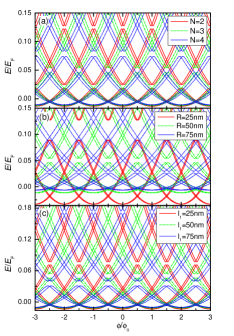
Figure 3: The electron energy levels in the mesoscopic polygon as a function of the magmatic flux $\phi$ in the presence of SOI with $\alpha=1.0\times 10^{-11}$ eVm. The parameters are the same sa Fig. 2.

The energy gaps $E_{{\normalsize g}}$ as functions of $l_{1}$ are plotted in Fig. 4 for no SOI. Panel (a) is for the energy gaps which are between the first energy level and the second energy level of the energy spectra in Fig. 2(c). The energy gaps, which are between the third energy level and the fourth energy level, are shown in panel (b). Clearly, the gaps $E_{{\normalsize g}}$ can be effectively modulated by the geometrical parameter of the mesoscopic polygon. On the whole, the profile of the curves is always increase first and then decrease. For the limit of $l_{1}\rightarrow 0$, the energy gaps is small and decrease to zero quickly. While for another limit of $l_{1}\rightarrow\infty$, the energy gaps is also small, which shows the geometrical twoness of the mesoscopic polygon. For different values of $R$, the curves of the energy gaps take the rightward shifts which are larger at large radius. This may be due to the competition between the radius $R$ and length $l_{1}$. If the radius $R$ increasing, a longer length of $l_{1}$ is needed to exhibit the property of regular polygon. In addition, because of the transmission and reflection by the geometrical potential, the electrons in the mesoscopic polygon has a more complex interference than that in the perfect ring. This can be seen from the energy gaps in panel (b) where there exit two vibrations.

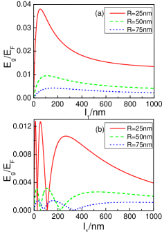
Figure 4: The relationship of the energy gaps in the mesoscopic polygon vs $l_{1}$ for $R=25$ nm, $50$ nm, $70$ nm at $N=3$ in the absence of SOI. (a) is for the energy gaps which are between the first energy level and the second energy level, and (b) is for the energy gaps which are between the third energy level and the fourth energy level.

For the energy gaps changing with the parameters $R$ or $N$, our calculations show the similar results as above, except for $R\rightarrow 0$ where the geometrical potential tends to infinite, i. e. $V_{{\normalsize g}}\rightarrow-\infty$, and the motions of electrons may be localized or isolated by these infinite potentials. So the energy gaps are increased to an finite value. The above-all mentioned behaviors can also be found for the energy gaps in the presence of Rashba SOI.

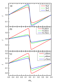
Figure 5: Persistent current in the mesoscopic polygon vs. magnetic flux $\phi$ at $\alpha=0$: (a) for $N=2$, $3$, $4$ at $R=50$ nm and $l_{1}=$ $50$ nm, (b) for $R=25$ nm, $50$ nm, $70$ nm at $N=3$ and $l_{1}=$ $50$ nm, (c) for $l_{1}=25$ nm, $50$ nm, $75$ nm at $N=3$ and $R=$ $50$ nm. The persistent current is in units of $E_{{\normalsize F}}/\phi_{0}$.

Now we proceed to investigate the persistent currents induced by the magnetic flux. At zero temperature, it is given by^[22]

$$I=-\mathrel{\mathop{\sum}\limits_{i\in{\normalsize occupied}}}\frac{\partial E_{i}}{\partial\phi},$$ (10)

where $E_{i}$ are the single particle eigenenergies. This formula is valid only in the absence of electron-electron interactions, which we neglect here.

For the given mesoscopic polygon with the filled lowest two bands, the persistent currents in the absence of SOI are calculated from the energy levels in Fig. 2 and shown in Fig. 5. We have known that the persistent current oscillations in a perfect ring have a sawtooth form at zero temperature. However, the mesoscopic polygon shows a smoothing of the oscillations. The smoothing and the swing of oscillation are decided not only by the gaps opened at the intersection points, but also by the geometrical structure of the mesoscopic polygon. We can see that the amplitude of oscillation, which is determined by the band width of the energy spectra, increases as the parameter $N$ increases and decreases as the radius $R$ and length $l_{1}$ increase.

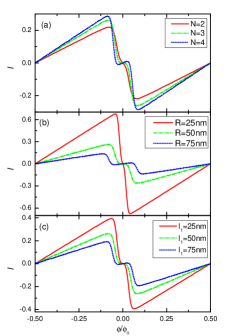
Figure 6: Persistent current in the mesoscopic polygon vs. magnetic flux $\phi$ in the presence of SOI with $\alpha=1.0\times 10^{-11}$ eVm. The parameters are the same as Fig. 5. The persistent current is in units of $E_{{\normalsize F}}/\phi_{0}$.

While the SOI is considered, the corresponding persistent currents are shown in Fig. 6 according to the energy spectra in Fig. 3. On the whole, the oscillation amplitude of persistent current is similar to the results without the SOI. While particularly, the oscillation in one period shows an additional small zigzag which is due to the energy-split induced by SOI seen in Fig. 3. As we increase the parameter $N$, the whole fluctuation range of the persistent current increases accordingly. However the whole fluctuation ranges decrease as the increscences of $R$ and $l_{1}$. While the increases in $N$, $R$ and $l_{1}$ will all broaden and enlarge the small zigzag.

In summary, we study the mesoscopic polygon with round corners and investigate the geometrical effects on the quantum behaviors of a single electron in it under the influences of magnetic flux. Different from the studies of other mesoscopic structures, the geometric potentials which can bring on the new phenomena have been considered in this new system. We calculate the electron states and persistent currents changing with magnetic flux $\phi$ under two circumstances, with SOI and without SOI, respectively. The geometrical structure results in an effective periodic potential and leads to a new electronic structure accompanying with the energy gaps. The changes of the gaps displays the geometrical twoness of the mesoscopic polygon. The SOI results in the split energy levels and induces the unique periodic structure for the persistent current which is formed by a large zigzag and a small zigzag in one period. We also find that the energy spectrum and the related physical properties can be modulated by the geometrical methods. It can be concluded that the rich structures in the mesoscopic polygon can provide more freedom to tailor the electronic structures and then effectively control the related properties. So we may construct the custom-built quantum device from the ring geometry to the polygon geometry, even build a geometrical supperlattice.

The authors thank Dr S. Zhao, L. Zhang, R. Liang, Y. Liu, and Z. Yao for helpful discussions. This work is supported by NSF of China under Grant No. 10374075. E. Zhang is also supported by the Doctoral Foundation Grant of Xi’an Jiaotong University (XJTU) No. DFXJTU2004-10 and by the NSF of XJTU (Grant No. 0900-573042).

References

References

- [1] A. Lorke, R. J. Luyken, A. O. Govorov, J. P. Kotthaus, J. M. Garcia, and P. M. Petroff, Phys. Rev. Lett. 84 2223 (2000).
- [2] S. Iijima, Nature (London) 354, 56 (1991).
- [3] R. Martel, H. R. Shea and P. Avouris, Nature (London) 398, 299 (1999).
- [4] S. Zhang, Phys. Lett. A 285, 207 (2001); S. Zhang, Phys. Rev. B 65, 235411 (2002); S. Zhang, S. Zhao, M. Xia, E. Zhang, and T. Xu, Phys. Rev. B 68, 245419 (2003); S. Zhao, S. Zhang, M. Xia, E. Zhang, and X. Zuo, Phys. Lett. A 331, 138 (2004);
- [5] L. Žutić, J. Fabian, and S. Das Sarma, Rev. Mod. Phys. 76, 323 (2004).
- [6] Yu. A. Bychkov and E. I. Rashba, Pis’ma Zh. Eksp. Teor. Fiz. 39, 66(1984) [JETP Lett. 39, 78(1984)].
- [7] T. Heinzel, K. Ensslin, W. Wegscheider, A. Fuhrer, S. Lüscher, and M. Bichler, Nature (London) 413, 822 (2001); B. Molnár, F. M. Peeters, and P. Vasilopoulos, Phys. Rev. B 69, 155335 (2004); X. F. Wang and P. Vasilopoulos, Phys. Rev. B 72, 165336 (2006); J. Splettstoesser, M. Governale, and U. Zülicke, Phys. Rev. B 68, 165341 (2003); J. S. Sheng and Kai Chang, Phys. Rev. B 74, 235315 (2006).
- [8] D. Bercioux, M. Governale, V. Cataudella, and V. M. Ramaglia, Phys. Rev. Lett. 93, 056802 (2004); D. Bercioux, M. Governale, V. Cataudella, and V. M. Ramaglia, Phys. Rev. B 72, 075305 (2005).
- [9] D. Bercioux, D. Frustaglia, and M. Governale, Phys. Rev. B 72, 113310 (2005).
- [10] M. J. van Veenhuizen, T. Koga, AND J. Nitta, Phys. Rev. B 73, 235315 (2006).
- [11] H. A. Ainspan and Keith A. Jenkins, IEEE JOURNAL OF SOLID-STATE CIRCUITS, 33, 2028 (1998).
- [12] A. V. Chaplik and R. H. Blick, New Journal of Physics 6, 33(2004).
- [13] R. C. T. da Costa, Phys. Rev. A 23, 1982 (1981).
- [14] H. Aoki, M. Koshino, D. Takeda, H. Morise, and K. Kuroki, Phys. Rev. B 65, 035102 (2002).
- [15] M. V. Entin, and L. I. Magarill, Phys. Rev. B 66, 205308 (2002).
- [16] S. Zhang, E. Zhang, S. Zhao, and M. Xia, Mod. Phys. Lett. B 18, 817 (2004).
- [17] A. Marchi, S. Reggiani, M. Rudan, and A. Bertoni, Phys. Rev. B 72, 035403 (2005).
- [18] E. Zhang, S. Zhang, and Q. Wang, Phys. Rev. B 75, 085308 (2007).
- [19] I. V. Blonskyy, V. M. Kadan, A. K. Kadashchuk, A. Y. Vakhnin, A. Y. Zhugayevych, and I. V. Chervak, Phys. Low-Dimens. Struct. 7-8, 25 (2003); O. Bisi, S. Ossicini, and L. Pavesi, Surf. Sci. Rep. 38, 1 (2000).
- [20] D. Mailly, C. Chapelier, and A. Benoit, Phys. Rev. Lett 70, 2020 (1993); T. Koga, Y. Sekine, and J. Nitta, Phys. Rev. B 74, 041302 (2006).
- [21] Y. V. Pershin and C. Piermarocchi, Phys. Rev. B 72, 125348 (2005).
- [22] M. Büttiker, Y. Imry, and R. Landauer, Phys. Lett. A 96, 365 (1983).