New insights into the stellar content and physical conditions of star-forming galaxies at $z=2-3$ from spectral modelling

Abstract

We have used extensive libraries of model and empirical galaxy spectra (assembled respectively from the population synthesis code of Bruzual and Charlot and the fourth data release of the Sloan Digital Sky Survey) to interpret some puzzling features seen in the spectra of high redshift star-forming galaxies. We show that a stellar He ii $\lambda 1640$ emission line, produced in the expanding atmospheres of Of and Wolf-Rayet stars, should be detectable with an equivalent width of $0.5-1.5$ Å in the integrated spectra of star-forming galaxies, provided the metallicity is greater than about half solar. Our models reproduce the strength of the He ii $\lambda 1640$ line measured in the spectra of Lyman break galaxies for established values of their metallicities. With better empirical calibrations in local galaxies, this spectral feature has the potential of becoming a useful diagnostic of massive star winds at high, as well as low, redshifts.

We also uncover a relationship in SDSS galaxies between their location in the [O iii]/H$\beta$ vs. [N ii]/H$\alpha$ diagnostic diagram (the BPT diagram) and their excess specific star formation rate relative to galaxies of similar mass. We infer that an elevated ionisation parameter $U$ is at the root of this effect, and propose that this is also the cause of the offset of high redshift star-forming galaxies in the BPT diagram compared to local ones. We further speculate that higher electron densities and escape fractions of hydrogen ionising photons may be the factors responsible for the systematically higher values of $U$ in the H ii regions of high redshift galaxies. The impact of such differences on abundance determinations from strong nebular lines are considered and found to be relatively minor.

1 Introduction

Table 1: Adopted emission-line luminosities of individual Wolf-Rayet stars in units of $10^{35}$ erg s^-1

Line name	WNE stars		WNL stars		OIf stars
	$Z<0.2Z_{\odot}$	$Z\geq 0.2Z_{\odot}$	$Z<0.2Z_{\odot}$	$Z\geq 0.2Z_{\odot}$
He ii $\lambda 4686$	1.7a	8.4	4.3	24.7	1.3
He ii $\lambda 1640$	17	84	43	247	20
N iii $\lambda 4640$	0	0	4.0	6.3	0
N v $\lambda 4603-4620$	0.24a	1.60	0	0	0

^a Includes binaries, see Crowther & Hadfield (2006).

The spectra of galaxies, particularly at optical and ultraviolet (UV) wavelengths, contain a wealth of information on their stellar populations and interstellar media. The veritable explosion in the size of galaxy surveys which we have witnessed in recent years has been accompanied by the development of increasingly sophisticated models for the analysis and interpretation of their spectra (e.g. Kewley et al. 2001a; Bruzual & Charlot 2003; Heavens et al. 2004; Ocvirk et al. 2006). The same analysis tools are also increasingly being applied to the spectra of galaxies at redshifts $z>1$, even though their detailed characteristics may well differ from those of their counterparts at lower redshifts. Considering, for example, star-forming galaxies, it now seems well established that at high redshifts a larger fraction of the star formation activity took place in conditions similar to those encountered today in the relatively rare ‘luminous infrared galaxies’ (e.g. Reddy et al. 2006 and references therein), and that the transition from starburst dominated to a more quiescent mode of star formation occurred at redshifts between $z\simeq 2$ and 1 (e.g. Papovich et al. 2005).

It is thus reasonable to question to what extent diagnostic tools developed to interpret local galaxies may need to be modified in order to decipher correctly the clues encoded in the spectra of high redshift galaxies. In this paper we use state-of-the-art spectral synthesis models and observations of local galaxies to investigate two apparent ‘anomalies’ which have been noted in the spectra of high redshift star-forming galaxies. The first is the common detection of the He ii $\lambda 1640$ emission line with a width which is suggestive of an origin in the expanding atmospheres of luminous stars rather than in H ii regions. This spectral feature is clearly seen in the composite rest-frame UV spectrum of more than 800 Lyman break galaxies at $z\simeq 3$ constructed by Shapley et al. (2003). As those authors point out, its strength is underestimated by continuous star formation models generated by the Starburst99 code (Leitherer et al. 1999), particularly at sub-solar metallicities. Locally, the He ii $\lambda 1640$ emission line is prominent in the UV spectra of starburst galaxies, but only during a brief period when the number of Wolf-Rayet (W-R) stars is at a maximum (e.g. Chandar, Leitherer & Tremonti 2004), so that its strength in the composite spectrum of hundreds of galaxies which span a wide range of ages, from $10^{7}$ to $10^{9}$ years (Shapley et al. 2001; Erb et al. 2006b), is at first sight puzzling. Here we reassess this ‘problem’ using the most recent models and observations of Wolf-Rayet stars in galaxies of differing metallicities, and taking into account a range of star formation histories.

The second issue concerns the indication that star-forming galaxies at $z\lower 2.15277pt\hbox{$\;\buildrel>\over{\sim}\;$}1$ may exhibit systematically higher ratios of collisionally excited to recombination lines than present-day H ii regions (Shapley et al. 2005; Erb et al 2006a; Kriek et al. 2007). Although the data samples are still small, most of the galaxies at $z\lower 2.15277pt\hbox{$\;\buildrel>\over{\sim}\;$}1$ where the relevant emission lines have been measured, are offset—relative to lower $z$ galaxies—in the [O iii]$\lambda 5007$/H$\beta$ vs. [N ii]/H$\alpha$ diagram first proposed by Baldwin, Phillips & Terlevich (1981, BPT) as a way of classifying emission line regions and their sources of ionisation/excitation. A variety of different physical processes may be at the root of such differences, as discussed by Shapley et al. (2005, see also Liu et al 2008); we investigate this question further here with detailed modelling and comparison with the large body of data on local galaxies provided by the Sloan Digital Sky Survey (SDSS).

Where relevant, we have adopted today’s consensus cosmology with density parameters $\Omega_{\rm M}=0.3$, $\Omega_{\Lambda}=0.7$ and a Hubble parameter $H_{0}=70$ km s^-1 Mpc^-1. We have also adopted throughout the stellar initial mass function (IMF) of Chabrier (2003), unless otherwise specified.

2 Origin of the He ii $\lambda 1640$ emission line in the integrated spectra of high redshift star-forming galaxies

2.1 Theoretical Models

We use as a starting point the spectral evolution models by Bruzual & Charlot (2003, BC03). We have adopted the Padova 1994 tracks (see BC03 for details) for the stellar evolution but use Geneva ’high-mass-loss’ tracks (Meynet et al. 1994) for the Wolf-Rayet phase. These provide a good match to the observational data and agree with tracks for stellar evolution which take into account the effects of stellar rotation (Meynet & Maeder 2005; Vazquez et al. 2007). For the work described in this paper, we have made one significant addition to the Bruzual & Charlot (2003) models by including the predictions of the strengths of UV and optical emission lines due to W-R stars from the stellar evolution models by Schaerer & Vacca (1998). It is important to emphasise here that the absolute calibration of the luminosity of the He ii $\lambda 1640$ line (of particular interest to our present investigation) is based on a still rather scant body of measurements. Schaerer & Vacca (1998) used reference luminosities for the optical He ii $\lambda 4686$ emission line from the best empirical compilations available a decade ago and then adopted appropriate scaling factors to predict the luminosity of the $\lambda 1640$ line (for WN stars; for WC and WO stars the reference line is C iv $\lambda 5808$). More recently, Crowther & Hadfield (2006) have reexamined these calibrations with a more comprehensive sample of W-R spectra and better corrections for reddening, and concluded that: (a) the He ii $\lambda 4686$ line has a higher luminosity in metal-poor WNE stars than the value adopted by Schaerer & Vacca (1998); (b) the ratio of the luminosities in the two He ii lines, $L(\lambda 1640)/L(\lambda 4686)$, is 20% larger than assumed by Schaerer & Vacca; and (c) there is a metallicity dependence, not only in the ratio of W-R to O-type stars, but also in the sense that W-R stars with lower metallicity have lower luminosity He ii lines.

We have modified the Schaerer & Vacca (1998) models as implemented in Starburst99 to reflect these changes in the overall calibrations of the He ii emission line luminosities. Specifically, for WN stars we have adopted the line luminosities listed in Table 1, while for WC stars we have retained the calibrations by Schaerer & Vacca (1998). Following Crowther & Hadfield (2006), we have made a distinction between stars with metallicities lower and higher than 1/5 solar (this being approximately the metallicity of the Small Magellanic Cloud). As discussed below we have also adopted the He ii $\lambda 4686$ luminosity for WN class 5–6 as representative of the WNL luminosity.

For OIf stars we have adopted the luminosities given in Table 1, kindly provided by P. Crowther (2007, priv.  comm). The inclusion of these stars does make a difference at very early stages in a starburst and particularly for low metallicities where the WR phase is much less prominent. At $Z=0.2Z_{\odot}$ the inclusion of OIf stars increases the He ii $\lambda 1640$ luminosity by $\sim 50$% and larger gains are seen at lower metallicities.

We have also adopted a ratio of 10 between the luminosity of He ii $\lambda 1640$ and He ii $\lambda 4686$ for both WNL and WNE stars. We then used Starburst99 to calculate single-stellar populations from these models, using the same IMF and stellar tracks as used by Bruzual & Charlot (2003). These single-stellar populations SSP were finally interpolated onto the same time grid as used by Bruzual & Charlot (2003) to allow the calculation of arbitrary star formation histories.

Even with these revisions, however, substantial uncertainties remain in the modelling. They have two separate causes: the association of observational data with theoretical models and the distribution of observed fluxes. The connection between observational data and theoretical tracks is non-trivial essentially because the observed features originate in the stellar wind and the models focus on the stellar interior. Thus spectroscopic classifications of WR stars do not necessarily map naturally onto the evolutionary model parameters — see for instance the discussion by Foellmi et al. (2003) and Meynet & Maeder (2003). Furthermore, the currently available libraries of stellar tracks (Meynet & Maeder 2003) do not include rotation (see Vazquez et al. (2003) for a partial implementation) and the population evolution modes do not include a binary channel (see however Han et al. 2007) which may be of crucial importance for Wolf-Rayet formation at low metallicity (Foellmi et al. 2003; Crowther 2007).

The second problem arises because there seems to be a wide spread in the luminosities of the He ii lines measured in W-R stars of even the same sub-type, and the available data are still too few to ascertain the form of the distribution function of, for example, $L(\lambda 4686)$ for a given W-R spectral type or sub-type (see Figure 2 of Crowther & Hadfield 2006). The luminosities span such a large range that any predictions are sensitive to the extreme, and hence rare, values. Thus, measurements in large samples of W-R stars—not yet assembled—are required to characterise the distribution adequately. This is indeed the reason why we have adopted the WN class 5–6 as representative of the WNL luminosity, since this is the best-sampled WNL class.

In summary, until more comprehensive observational libraries and further theoretical work on the line fluxes in W-R stellar atmospheres become available, we have to accept the fact that even the best evolutionary synthesis models probably cannot predict the luminosities of W-R emission lines with an accuracy better than a factor of $\sim 2$–$3$ (based on the empirical spread of the luminosities of these lines and differences in mapping between empirical data and evolutionary models).

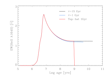
Figure 1: Time evolution of the equivalent width of the He ii $\lambda 1640$ emission line for three different star formation histories. The black line is for a continuous star formation model in which the star formation rate declines slowly, with an $e$-folding time $\tau=15$ Gyr. The blue line is for a faster decline ($\tau=1$ Gyr), while the red line is for a single burst of star formation at a fixed rate and lasting 1 Gyr, after which the star formation abruptly ceases.

2.2 Synthesising the He ii $\lambda 1640$ emission line: simple star formation histories

With these limitations in mind, we now consider the strengths of the He ii $\lambda 1640$ lines generated by our grid of models. As a general consideration we recall that only the hottest stars (or a power-law continuum as produced for example by an active galactic nucleus) can photoionize He⁺ to create nebular He ii emission since this requires photons with energies in excess of 54.4 eV. However both early O supergiants and Wolf-Rayet stars have sufficient numbers of photons with energy above 24.6 eV to create stellar He ii emission.

Given the short lifetimes of these stars, the stellar He ii $\lambda 1640$ line would be present for only a few Myr following a burst of star formation. However in the more realistic case of a protracted star formation episode, this narrow ‘step-function’ becomes smoothed out, as we now explore.

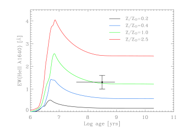
Figure 2: Time evolution of the equivalent width of the He ii $\lambda 1640$ emission line for four difference metallicities, as indicated. All four curves refer to the model with slowly declining star formation rate ($\tau=15$ Gyr). The dot at $\log t=8.5$ is the value of EW(He ii $\lambda 1640$) measured from the composite spectrum of 811 Lyman break galaxies published by Shapley et al. (2003), while the error bar shows the inter-quartile range of their ages (Shapley et al. 2001). The measured value of EW(He ii $\lambda 1640$) is reproduced by our models with metallicities $\mathbf{Z=0.75-1.5\,Z_{\odot}}$, somewhat higher than, but still consistent with, current estimates of the metallicity of LBGs.

Figure 1 illustrates the time evolution of the equivalent width of the He ii $\lambda 1640$ emission line for three different star formation histories. The black line shows the case of a nearly constant star formation rate (approximated by an exponentially declining rate of star formation with a very long decay time of 15 Gyr); the blue line is for a more rapidly declining star formation rate ($\tau=1$ Gyr); and the red line is for a discrete burst of star formation at a constant rate lasting 1 Gyr (after which the star formation is abruptly switched off). For the moment we keep the metallicity constant at the solar value.

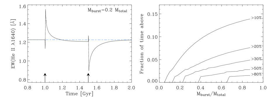
Figure 3: Left panel: An illustration of the effect of a burst of star formation on the equivalent width of the He ii $\lambda 1640$ emission line. The burst is superimposed on an underlying level of near-constant star formation which gives EW($\lambda 1640)\simeq 1.2$ Å (shown by the horizontal short-dash line). At $t_{\rm sf}=10^{9}$ years, a burst of duration 5$\times 10^{8}$ years, building up 20% of the stellar mass, is superposed (the arrows indicate the start and end of burst). Right panel: The effect on EW($\lambda 1640$) of a burst of star formation superposed on a pre-existing stellar population forming stars at a constant rate. The $x$-axis shows the strength of the burst, as measured by the fraction of stellar mass contributed by the burst to the final total stellar mass. The $y$-axis shows the fraction of time that the EW($\lambda 1640$) is increased by a given percentage (indicated at the right of each curve) above the value for constant star formation.

These three examples were chosen to illustrate star formation histories which may be appropriate to composite spectra of many galaxies (such as the LBG average constructed by Shapley et al. 2003) where the individual characteristics of the component spectra are smoothed out. These models are therefore not applicable to individual galaxies, caught at a particular stage in their evolution. It is worth pointing out here that during short bursts of star formation, EW(He ii $\lambda 1640$) can reach values two to three times higher than those shown in Figure 1; such models would be able to reproduce the observations of He ii $\lambda 1640$ in individual star-forming galaxies at low (e.g. Gonzalez-Delagado et al. 1999; Leitherer et al. 2002; Chandar et al. 2004), as well as high (e.g. Lowenthal et al. 1997; Kobulnicky & Koo 2000), redshifts.

Returning to Figure 1, it can be seen that in all three cases shown, the equivalent width of the He ii emission line reaches a peak value only a few million years after the onset of star formation, when the number of W-R stars is at a maximum. While this behaviour was expected, what has perhaps not been fully appreciated until now is that, following this W-R bright phase, the quantity EW($\lambda 1640$) settles to a plateau value of $\simeq 1.5$ Å which is maintained until the star formation rate essentially stops. The physical reason for this plateau is that the underlying UV continuum at 1640 Å is also due to massive stars with short evolutionary timescales (albeit not as massive, nor as short-lived as the W-R stars, the luminosity-weighted $T_{\mathrm{eff}}$ at $\lambda=1640$ Å is 25,000 K) rather than being set by the previous, longer-term, star formation history. Thus the ratio between the luminosity in the He ii emission line and in the continuum—which the EW measures—tends to a constant value after about $10^{8}$ years, when the number of OB stars has stabilised.

Next we consider the effect of metallicity on the predicted value of EW($\lambda 1640$), limiting ourselves to the slowly declining star formation rate case with $\tau=15$ Gyr. As can be readily appreciated from Figure 2, while the general form of the time evolution of EW($\lambda 1640$) is common to all four values of metallicity considered (from $Z=2.5\,Z_{\odot}$ to $Z=1/5\,Z_{\odot}$), the peak and plateau values of EW($\lambda 1640$) depend sensitively on metallicity, in the sense that the He ii emission line is considerably weaker at subsolar metallicities (and stronger when $Z>Z_{\odot}$). Such a marked dependence is due to two effects. First, and most important, the number of massive stars which evolve to the W-R stage is substantially reduced at sub-solar metallicities, as evidenced by the reduced ratio of W-R to O-type stars—as well as the change in the W-R sub-type distribution—between the Milky Way and the Magellanic Clouds (e.g. Crowther 2007 and references therein). Second, as mentioned above, there is evidence that in individual W-R stars of a given sub-type the luminosity of the He ii lines is lower at lower metallicities (Crowther & Hadfield 2006). The metallicity dependence of the winds from the W-R progenitors is presumably at the root of these differences (Vink & de Koter 2005).

Also shown in Figure 2 is the value EW($\lambda 1640)=1.3\pm 0.3$ Å measured from the composite of spectrum of 811 Lyman break galaxies published by Shapley et al. (2003). In order to measure the equivalent width, we normalised the spectrum according to the prescription by Rix et al. (2004); the error quoted reflects the uncertainties in both the continuum placement and the width of the emission line. From our models, this value of EW($\lambda 1640$) is that expected for star-forming galaxies where star formation has been progressing for longer than $\sim 100$ Myr and the metallicity is roughly between 0.75 and 1.5 times solar. For comparison, we estimate that the typical metallicity of the Lyman break galaxies in the composite of Shapley et al. (2003) is in the range $Z_{\rm LBG}\simeq 0.3-1Z_{\odot}$, based on the determinations by Pettini et al. (2001) and Erb et al. (2006a; see also Appendix A), while their median age is $\sim 320$ Myr (Shapley et al. 2001). Thus, while the models seem to underestimate somewhat the equivalent width of the He ii $\lambda 1640$ emission line, it is nevertheless encouraging that they come so close, given the current uncertainties in the absolute calibrations of the luminosities of the He ii lines, as emphasised above. We also point out that our models match simultaneously the equivalent width of the C iv $\lambda 1550$ P-Cygni line, unlike previous attempts to account for the He ii $\lambda 1640$ emission by appealing to a top-heavy IMF (e.g.  Shapley et al. 2003; Chandar et al. 2004). Furthermore, in our models the luminosity-weighted width of the optical He ii $\,\lambda 4686$ line of $\sim 1500$–$2000$ km s^-1. A similar width is expected for He ii $\lambda 1640$, in good agreement with the FWHM($\lambda 1640$) $\sim 1500$ km s^-1 of this spectral feature in the Shapley et al. (2003) composite spectrum. This gives added confidence to the identification of this line as originating in the winds of W-R and OIf stars.

2.3 The effect of bursts of star formation

We now briefly consider the effect on the equivalent width of the He ii $\lambda 1640$ line of a less simplistic model for the star formation activity, by adding a burst of star formation to an underlying continuous mode. We illustrate this composite scenario in the left panel of Figure 3, where the burst is introduced as a step function at time $t_{\rm sf}=1$ Gyr and lasts for 0.5 Gyr. The underlying continuous mode is, as before, a slowly declining one with $\tau=15$ Gyr, and the strength of the burst is such that it accounts for 20% of the stellar mass of the system at the end of the burst.

Referring to the figure, we see that, following the burst, the equivalent width EW($\lambda 1640$) increases by about 25% due to the enhanced contribution from the Of and W-R stars created in the burst. It subsequently declines to the pre-burst value on a timescale of $\sim 200$ Myr as the contribution to the continuum from lower-mass O and B-type stars without a He⁺ zone grows. After the end of the burst, at $t_{\rm sf}=1.5$ Gyr, the EW drops until all the massive stars formed in the burst have faded away, and then rises back to the pre-burst equilibrium value. The decline in EW after the start of the burst and its increase after the end of the burst have the same shape because the same stellar populations contribute (with the same timescales) in both cases.

The features seen in Figure 3 are generic to this kind of composite scenario, although the details would change with the exact parameters of the burst (and the sharp transitions in Figure 3 would of course be smoothed out if one considered a series of bursts or smoother onset/termination of star formation). The important point, however, is that, while bursts of star formation do have an effect on the equivalent width of the He ii $\lambda 1640$ line, the effect is relatively modest and short-lived. We quantify this conclusion in the right-hand panel of Figure 3 which shows the fraction of time during which the quantity EW($\lambda 1640$) is increased by a given percentage over the equilibrium value following the onset of a 500 Myr long burst of star formation. The effect is at the $20-30$% level for less than 10% of time (that is, for less than 50 Myr); higher perturbations are even more short-lived. Such variations are small compared with the more important uncertainty in the overall calibration of the luminosity of the He ii lines resulting from the poor empirical sampling of the spectra of W-R stars in nearby galaxies. Of course, the increase in EW($\lambda 1640$) following a burst can be made larger by increasing the contrast of the burst over the underlying continuous star formation activity (see right-hand panel of Figure 3). Thus, if a strong burst takes place after a period of low star formation activity (lasting longer than the lifetimes of the OB stars contributing to the UV continuum), then the increase in EW($\lambda 1640$) will be much larger than the $\sim 25$% increase appropriate to the model shown in Figure 3. Nevertheless, even in these circumstances, the period during which EW($\lambda 1640$) is abnormally high is brief, and the equivalent width of the line settles to the equilibrium value on a $\sim 10^{8}$ year timescale.

Summarising the conclusions of this section, our models show that the presence of a detectable He ii $\lambda 1640$ emission line in the spectra of galaxies actively forming stars need not be surprising and requires no exotic stellar populations (cf. Jimenez & Haiman 2006). Provided the metallicity is higher than about half solar, we expect that this emission line should have an equivalent width EW($\lambda 1640)\sim 0.5$ Å or greater while star formation is proceeding. The equivalent width settles to an equilibrium value because its value is determined from stars at the upper end of the initial mass function; perturbations from this equilibrium value are short-lived because they are determined by a temporary excess, or deficit, of Of and W-R stars compared to O and early B stars. For this same reason, EW($\lambda 1640$) responds sensitively to changes in metallicity, since it is the metallicity that apparently determines the ratio of W-R to O stars and, to a lesser extent, the luminosity of the He ii $\lambda 1640$ line in a given W-R star. Considering the paucity of current data on the strength of this emission line in stars of different W-R sub-types and metallicities, it is perhaps fortuitous that our models reproduce within a factor of $\sim 2$ the value of EW($\lambda 1640$) in the composite spectrum of Lyman break galaxies at $z\simeq 3$, for current estimates of their metallicities. Nevertheless, the agreement is encouraging. There are good prospects that, as more data are gathered on the luminosity $L(\lambda 1640)$ in local galaxies with different metallicities and star formation histories, we may be able to use the He ii line to investigate the properties of stellar winds in galaxies at high redshifts.

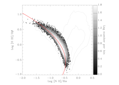
Figure 4: The BPT diagram of actively star-forming galaxies from the SDSS DR4. The number of galaxies in each bin of $\log$ [O iii]/H$\beta$ vs. $\log$ [N ii]/H$\alpha$ is shown on a logarithmic grey scale indicated on the right of the diagram. The analytic fit to the red ridge line is given by eq. (1) (see text). The dotted contours enclose, respectively, 5, 10, 20, 50, 90 and 99% of all galaxies in DR4 (in all three classes: Star-Forming, AGN, and Composite) in which the four emission lines are detected at a greater than $5\sigma$ significance level.

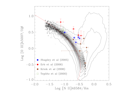
Figure 5: SDSS and high redshift galaxies in the [O iii]/H$\beta$ vs. [N ii]/H$\alpha$ diagnostic diagram. Galaxies at $z>1$ are from the sources indicated in the lower left-hand corner of the diagram. The grey scale used here to represent the SDSS galaxies was constructed by normalising the distribution function in bins along the $x$-axis, so that the total number of galaxies in each bin is the same. This representation has the advantage of bringing out more clearly the structure of the locus occupied by star-forming galaxies in the SDSS. Contours are as in Figure 4.

3 The [O iii] $\lambda 5007$/H$\beta$ vs. [N ii]$\lambda 6583$/H$\alpha$ diagram at low and high redshift

Since the seminal paper by Baldwin et al. (1981), this diagnostic diagram has been used extensively to separate star forming galaxies from LINERS, Seyfert 2 galaxies, and mixed AGN/stellar ionisation systems (e.g. Veilleux & Osterbrock 1987; and, more recently, Kauffmann et al. 2003; Brinchmann et al. 2004 among many others).

In order to compare galaxies at high redshift with local ones, we use the fourth data release (DR4) of the SDSS (Adelman-McCarthy et al. 2006; York et al. 2000). SDSS spectra were obtained using a fibre spectrograph with 3 arcsec wide fibre apertures and we re-analyse the galaxy spectra with the pipeline reduction described by Tremonti et al. (2004). In this sample stellar masses were derived using the precepts of Kauffmann et al. (2003), and strong-line oxygen abundances and star formation rates determined with the Bayesian method discussed by Brinchmann et al. (2004). The overall properties of this sample are similar to those of the smaller SDSS DR2 sample of Brinchmann et al. (2004), whose criteria we have adopted to classify the galaxy emission line spectra as dominated by star formation (the SF class), AGN, or a mix of the two (the Composite class). Here we limit ourselves to galaxies in the SF class, which are plotted on the BPT diagram in Figure 4; we have included all galaxies in which the four emission lines in question are detected with a signal-to-noise ratio $S/N>5$; there are 85748 galaxies in DR4 satisfying these criteria. We elected not to consider the Composite class because a secure identification of the main ionisation mechanism can only be made for a small subset of objects in that class. However, Liu et al. (2008) have examined these more extreme galaxies in a recent analysis which complements that presented here.

A notable feature of the BPT diagram is that star-forming galaxies fall in a narrow region of the [O iii]/H$\beta$ vs. [N ii]/H$\alpha$ plane, around a ridge line well represented by the quadratic equation:

$$x=-0.596y^{2}-0.687y-0.655$$ (1)

where $x=\log$ [N ii]/H$\alpha$ and $y=\log$ [O iii]/H$\beta$. In determining this best-fit line we have excluded galaxies with stellar mass surface density $\mu_{\star}>3\times 10^{8}\,M_{\odot}$ kpc^-2. Such high stellar mass surface densities are characteristics of luminous bulges; as shown by Kauffmann et al. (2003), their removal from the sample is effective in excluding galaxies with low levels of AGN activity.

As mentioned in the Introduction, star-forming galaxies at $z\lower 2.15277pt\hbox{$\;\buildrel>\over{\sim}\;$}1$ seem to be offset significantly from this ridge line. Although all four emission lines have been measured in only a handful of high redshift galaxies so far (due to the limitations of current near-infrared spectrographs), the offset from the large body of SDSS measurements is readily apparent in Figure 5. This offset can be quantified with two parameters: the distance along the ridge line defined by eq. (1), $d_{\rm A}$ (defining arbitrarily the zero point to be at $x_{0}=-0.61$, $y_{0}=-1.1$), and the distance perpendicular to the ridge line, $d_{\rm P}$. The high redshift galaxies included in Figure 5 are UV-luminous galaxies at $z\simeq 2.2$ from Erb et al. (2006a), selected according to the ‘BX’ criteria of Steidel et al. (2004), and including unpublished data for Q2343-BX474 (Erb 2007, priv. communication); the star-forming galaxies at $z=2.0-2.6$ from the $K$-band selected sample studied by Kriek et al. (2007), excluding those classified as AGN; the star-forming galaxies at $z=1.0-1.5$ from the DEEP2 galaxy redshift survey observed by Shapley et al. (2005); and the gravitationally lensed $z=2.7276$ Lyman break galaxy MS 1512–cB58 (Teplitz et al. 2000). This still meagre sample will undoubtedly increase significantly in the near future (e.g. Liu et al 2008), as the multi-object and multi-band capabilities of near-IR spectrographs on large telescopes improve. The purpose of our investigation here is to identify the physical processes which are responsible for the offset of high-$z$ galaxies in the BPT diagram.

3.1 Star formation history and the BPT diagram

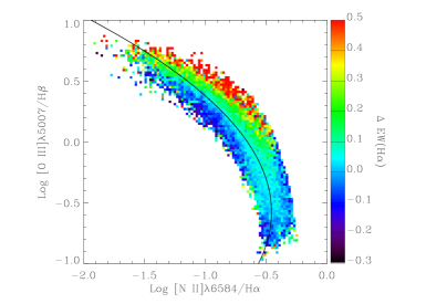
Figure 6: Variation of $\Delta{\rm EW(H}\alpha)$ in the BPT plane. The parameter $\Delta{\rm EW(H}\alpha)$, which measures the excess or deficit H$\alpha$ equivalent width compared to galaxies of similar mass, is clearly related to the distance of a galaxy from the ridge line (shown here in black).

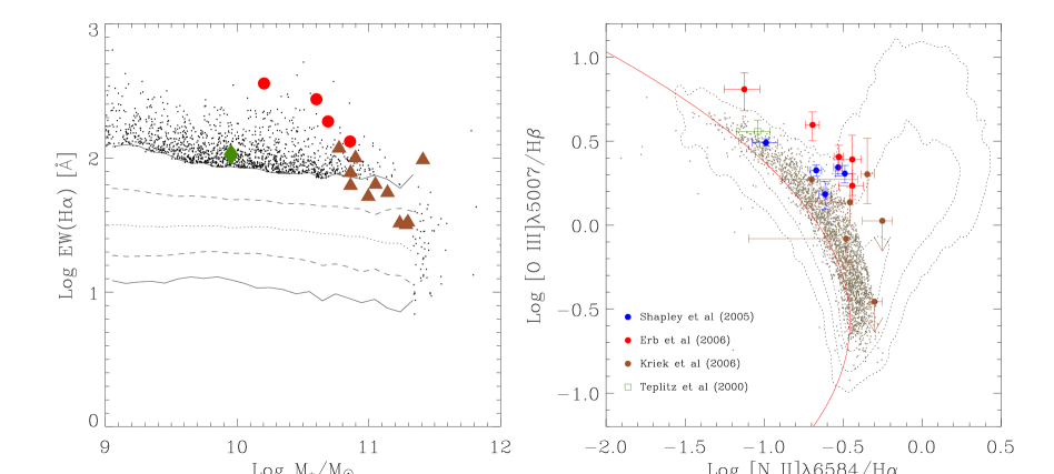
Figure 7: Left panel: The equivalent width of the H$\alpha$ emission line as a function of stellar mass. The dotted line shows the median trend for SDSS DR4 star forming galaxies. The dashed and continuous lines enclose respectively 68% and 95% of the galaxies. The lines have been drawn by binning galaxies in intervals of stellar mass chosen so that each bin includes 2500 galaxies. Galaxies at the extremes of the distribution, that is with values of EW(H$\alpha$) above the 97.5% limit and with stellar masses $M_{\star}>2\times 10^{11}\,M_{\odot}$ are plotted individually with small black dots. Coloured symbols refer to high redshift galaxies, as indicated in the legend in the right hand figure. The solid triangle at $\log M_{\star}/M_{\odot}\simeq 10$ shows the location of the galaxy MS 1512-cB58. Right panel: Location on the BPT diagram of: (a) the SDSS galaxies plotted individually with small dots in the left panel, and (b) the high redshift galaxies. Red ridge line and contours as in Figures 4 and 5.

With the large number of galaxies made accessible by the SDSS, it is possible to assess empirically how different galaxy properties, such as stellar mass, stellar surface density, age, metallicity and star formation rate map onto the [O iii]/H$\beta$ vs. [N ii]/H$\alpha$ plane. We have examined trends for a number of such quantities (Charlot et al. 2008, in preparation) and found the most relevant one for our purposes here to be the equivalent width of the H$\alpha$ emission line. It is not sufficient, however, simply to examine how EW(H$\alpha$) varies with the diagnostic ratios in the BPT diagram, in isolation from other physical parameters. Rather, it is more instructive to consider EW(H$\alpha$) differentially relative to other ‘similar’ galaxies, where the meaning of ‘similar’ depends on the issues under investigation (see, for example, the discussion in Kauffmann et al. 2006).

In our case, the equivalent width of the H$\alpha$ emission line is closely related to the specific star formation rate, (SFR/$M_{\star}$, where $M_{\star}$ is the assembled stellar mass), and both quantities then obviously depend on $M_{\star}$ (Brinchmann et al. 2004). In addition, there is also a small residual trend between EW(H$\alpha$) and $d_{A}$ at fixed $M_{\star}$. We removed the dependency on stellar mass and $d_{A}$ by calculating for each galaxy the difference $\Delta{\rm EW(H}\alpha)=\log{\rm EW(H}\alpha)-\log\langle{\rm EW(H}\alpha)\rangle$ where $\langle{\rm EW(H}\alpha)\rangle$ is the median value of the H$\alpha$ equivalent width in galaxies of the same mass and $d_{A}$. Thus the quantity $\Delta$EW(H$\alpha$) measures the excess, or deficit, of star formation activity in a galaxy relative to the value typical of similar galaxies. Mapping $\Delta$EW(H$\alpha$) onto the [O iii]/H$\beta$ vs. [N ii]/H$\alpha$ plane by means of colour-coding, as in Figure 6, shows very clearly that $\Delta$EW(H$\alpha$) is correlated with $d_{\rm P}$, the offset from the ridge line given by eq. (1).

Since our focus here is on empirical trends, we have chosen to concentrate on the equivalent width of the H$\alpha$ line. But we have also verified that as long as average trends are taken out as above, the star formation rate (SFR), the specific star formation rate (SFR/$M_{\star}$), and the star formation rate per area (SFR/Area), all show trends with position in the BPT diagram which are similar to that of $\Delta$EW(H$\alpha$), and with similar correlation strengths. We have also established that there is no trend between $\Delta$EW(H$\alpha$), defined as above, and the metallicity of the galaxies in the range $7.2<12+\log\textrm{O/H}<8.5$, where the oxygen abundance can be determined directly from consideration of temperature sensitive emission lines (the $T_{\rm e}$ method).

The pattern revealed by Figure 6 strongly suggests that the high redshift galaxies lying well above the ridge line in Figure 5 are experiencing unusually high levels of star formation for their stellar mass compared to most local galaxies. This interpretation is further strengthened by consideration of Figure 7, where we see that the galaxies at $z>1$ lie at, or beyond, the extremes of the locus of values in the EW(H$\alpha$) vs. $M_{\star}$ plane occupied by SDSS galaxies. [We could not include the measurements of DEEP2 galaxies by Shapley et al. (2005) in the left panel of Figure 7 because those authors did not publish values of EW(H$\alpha$)]. It is quite remarkable that the cut in EW(H$\alpha$) at a given mass, which involves no line ratios, has such a close correspondence on the position of the galaxies in the BPT diagram which only uses line ratios. We interpret this as evidence of a connection between star formation activity and the physical parameters determining the ratios of collisionally excited to recombination lines in the H ii regions.

3.2 Interpretation

In this section we explore further the connection between the specific star formation rate and the displacement from the ridge line in the BPT diagram which we uncovered in the preceding section. Theoretical modelling of nebular emission from star-forming galaxies (e.g. Charlot & Longhetti 2001; Kewley et al. 2001a) shows that a shift upwards in the BPT diagram can be achieved by increasing either the ionisation parameter $U$ (which in the usual definition is the ratio of the volume densities of ionising photons and particles) or the dust-to-metals ratio, which measures the degree to which heavy elements are depleted from the gas phase and which Charlot & Longhetti (2001) denote with symbol $\xi_{\rm d}$ (or both).

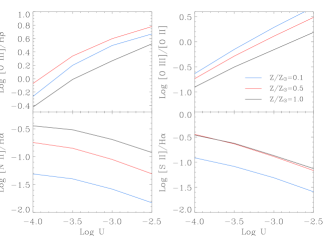
Figure 8: Dependence of four diagnostic line ratios on the ionisation parameter $U$. Different colours correspond to different metallicities $Z$, as indicated.

We have used the models of Charlot & Longhetti (2001) to illustrate the dependence of four emission line ratios on the ionisation parameter $U$ in Figure 8; three representative values of metallicity $Z$ are considered. As is well known, the [O iii]/H$\beta$ ratio increases with increasing $U$, while [N ii]/H$\alpha$ decreases (left-hand panels in Figure 8); the strong dependence of the latter on the metallicity partly helps to resolve the metallicity-ionisation parameter degeneracy in the BPT diagram. Also well understood (e.g. Penston et al. 1990) are the strong dependence of the [O iii]/[O ii] ratio on $U$, with metallicity $Z$ being a second-order effect, and the decrease of the ratio [S ii] $\lambda\lambda 6716,6731$/H$\alpha$ with increasing $U$ (right-hand panels in Figure 8). The dependence of the same four emission line ratios on the dust-to-metals ratio is, by comparison, much weaker (Figure 9); in general the parameter $\xi_{\rm d}$ is less important than either $U$ or $Z$ in determining the values of the four emission line ratios considered.

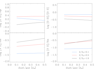
Figure 9: Dependence of four diagnostic line ratios on the dust-to-metals ratio $\xi_{\rm d}$; the ionisation parameter was kept fixed at $\log U=-3.5$. Different colours correspond to different metallicities $Z$, as indicated.

What is instructive is to consider the behaviour of the same four line ratios as a function of the H$\alpha$ equivalent width offset $\Delta{\rm EW(H}\alpha)$. To this end, we have binned the SDSS DR4 galaxies (class SF) by metallicity and in bins of $\Delta{\rm EW(H}\alpha)$; each bin includes 250 galaxies. We have excluded galaxies with $d_{\rm A}<1$ in order to avoid AGN contamination at the base of the AGN plume in the BPT diagram. Figure 10 shows that the behaviour of the four line ratios in response to changes in $\Delta{\rm EW(H}\alpha)$ is very similar to the response to changes in $\log U$, pointing to a close connection between $\Delta{\rm EW(H}\alpha)$ and the ionisation parameter. If one were to take the [O iii]/[O ii] ratio as a measure of $U$, as is often done, it would then be difficult to escape the conclusion that $U$ and $\Delta{\rm EW(H}\alpha)$ are correlated. The trends in Figure 10 also rule out a major contribution to the emission line ratios from shocks (Dopita & Sutherland 1995). While we cannot make the same rigourous statement for the high redshift galaxies, their locations in the BPT diagram are not consistent with significant shock contributions (e.g. see Figure 2 of van Dokkum et al. 2005).

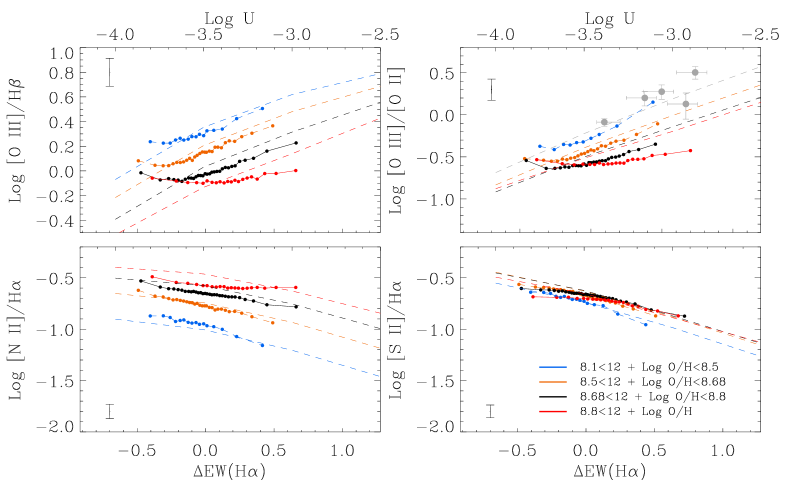
Figure 10: Observed dependence of the four diagnostic line ratios on the H$\alpha$ equivalent width offset $\Delta{\rm EW(H}\alpha)$ in four different metallicity ranges, as indicated. For comparison, the dashed lines show the expected dependence of the emission line ratios on the ionisation parameter $U$ (given on the top $x$-axes), calculated using the Charlot & Longhetti (2001) models. The vertical bar in each panel indicates the $\pm 1\sigma$ spread of the 250 galaxies in each bin about the median value plotted. The spread is generally larger than the observational uncertainties and insensitive to the bin size adopted; we thus consider it to be a real spread in the emission line ratios at a given value of $\Delta{\rm EW(H}\alpha)$. In the top right-hand panel we have included (filled grey dots) the Lyman break galaxies in which Pettini et al. (2001) measured both [O iii] $\lambda 5007$ and [O ii] $\lambda 3727$. The values of [O iii] $\lambda 5007$/[O ii] $\lambda 3727$ plotted here include a correction for dust appropriate to SDSS galaxies with similar metallicity (0.71), and we estimated EW(H$\alpha$) from the values of EW(H$\beta$) given by Pettini et al. (2001) using the average ratio EW(H$\alpha$)/EW(H$\beta$) for star-forming galaxies in the SDSS (4.69).

We have already seen (section 3.1 and Figure 6) that the quantity $\Delta{\rm EW(H}\alpha)$ determines where a galaxy falls in the BPT diagram relative to the ridge line of ‘normal’ star-forming galaxies. It therefore seems at least plausible (although the argument is indirect) that the offset of the high redshift star-forming galaxies in the BPT diagram is a reflection that their H ii regions are characterised by higher ionisation parameters than those of local galaxies in the SDSS survey. Liu et al. (2008) reached a similar conclusion for their smaller sample of more extreme SDSS galaxies. A higher ionisation parameter is certainly consistent with the high [O iii]/[O ii] ratios exhibited by the $z\sim 3$ LBGs observed by Pettini et al. (2001), shown with grey dots in the top right panel of Figure 10. Adopting this inference as a working assumption, we now proceed to consider which physical parameters may be responsible for the higher values of $U$.

3.3 Possible reasons for a higher ionisation parameter

We first consider the case where the H ii regions are ionisation bounded (this assumption will be relaxed later). The ionisation parameter at the edge of the effective Strömgren sphere can then be written as (e.g. Charlot & Longhetti 2001):

$$U(t)\propto\left[Q(t)\,n_{\rm H}\,\epsilon^{2}\right]^{1/3}$$ (2)

where $Q(t)$ is the rate of hydrogen ionising photons (s^-1), $n_{H}$ is the number density of hydrogen (cm^-3), and $\epsilon$ is the volume-filling factor of the gas (i.e. the ratio of the volume-averaged hydrogen density to $n_{\rm H}$). Thus, an increase in $U$ can have one of three sources, which we now consider in turn. Specifically, we have calculated the effects on relevant emission line ratios of altering the parameters $Q(t)$, $n_{\rm H}$ and $\epsilon$; in order to do so, we have combined the output of our population synthesis models described in Section 2.1 with the photoionisation code cloudy (version 07.02—Ferland et al. 1998).

3.3.1 Rate of ionising photons

The rate of ionising photons for a stellar population is a function of the composite stellar spectrum at ultraviolet wavelengths, which in turn depends on the mix of stellar spectral types that contribute. Thus, while there may be short-term fluctuations due to the evolutionary timescales of stars of different masses, in the case of continuous star formation the parameter $Q(t)$ quickly reaches an equilibrium value.

In our case, what is important is the ratio of photons that can ionise O⁺ to the hydrogen ionising photon; for an instantaneous burst, this ratio decreases with time after the burst, except for a brief increase during the Wolf-Rayet phase. However, in the case of a more protracted star formation episode, the ratio settles to a constant value. Figure 11 shows that even in the case of a relatively short-lived burst of star formation, lasting only 50 Myr, temporary fluctuations in the value of the parameter $d_{\rm P}$ (which we recall measures the offset perpendicular to the ridge line given by eq. 1) are washed out, so that $d_{\rm P}$ varies little with time until the end of the burst when it suddenly drops. The majority of this change in $d_{\rm P}$ is due to a change in the [O iii]/H$\beta$ ratio. The fact that even within an H ii region stars are not all strictly coeval will further smooth out the response of $d_{\rm P}$ to short-lived phases of stellar evolution.

The situation is analogous to that already discussed in Section 2.3 when we modelled the He ii $\lambda 1640$ emission line. Our modelling shows that the effects of bursts on $d_{\rm P}$ and [O iii]/H$\beta$ are even smaller than on EW($\lambda 1640$). Only when observing an H ii region at a very special time, such as 1 Myr after the onset star formation, do we expect to find elevated values of $d_{\rm P}$, but this possibility is implausible when considering the integrated spectrum of a whole galaxy.

Of course, an obvious way to increase the [O iii]/H$\beta$ ratio is to appeal to a change in the initial mass function: if we arbitrarily increased the relative numbers of the most massive stars, a harder far-UV spectrum would be produced. However, so far no direct evidence has been found for such a change in the IMF in high redshift star-forming galaxies. In the few cases where they have been recorded at sufficient signal-to-noise ratio, the details of their UV spectra are well reproduced by models with a Salpeter slope for stellar masses in excess of $\sim 10\,M_{\odot}$ (e.g. Pettini et al. 2000; Steidel et al. 2004; Erb et al. 2006a).

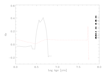
Figure 11: Time evolution of the parameter $d_{\rm P}$ (which measures the offset perpendicular to the ridge line in Figure 5) following an instantaneous burst of star formation (continuous line) and a burst of constant star formation lasting 50 Myr (dashed line). The models shown here are for solar metallicity. The arrows indicate the values of $d_{\rm P}$ appropriate to the $z>1$ star-forming galaxies in Figure 5.

3.3.2 Hydrogen density

Next we investigate the possibility that the higher ionisation parameter in high redshift star-forming galaxies (our working assumption) is due to higher densities of their H ii regions. We can address this point using the well known dependence on the electron density, $n_{\rm e}$, of the ratio of the S⁺ emission lines, [S ii] $\lambda 6716$/[S ii] $\lambda 6731$, which varies from $\sim 1.5$ to $\sim 0.5$ as $n_{\rm e}$ increases from 1 to $10^{4}$ cm^-3 (Osterbrock 1989).

In the left-hand panel of Figure 12 star-forming galaxies from the SDSS DR4 have been colour coded according to their [S ii] $\lambda 6716$/[S ii] $\lambda 6731$ ratio which clearly differentiates them in the BPT diagram, even though the ratio apparently varies by only a small fraction of the allowed range, from [S ii] $\lambda 6716$/[S ii] $\lambda 6731=1.5$ to 1.3. Within this restricted range, galaxies with smaller ratios (higher $n_{\rm e}$) are preferentially found above the ridge line defined by equation (1). It is therefore no surprise that an inverse correlation between [S ii] $\lambda 6716$/[S ii] $\lambda 6731$ and the parameter $d_{\rm P}$ is evident in the right-hand panel of Figure 12. We constructed this plot by calculating the median [S ii] $\lambda 6716$/[S ii] $\lambda 6731$ ratio in bins of $d_{\rm P}$ such that each bin included 1000 galaxies. Again we have excluded galaxies with $d_{\rm A}<1$ in order to avoid AGN contamination. Although the trend between the median values is clear-cut, we note that there is a substantial spread, of the order of $\pm 0.1$ dex (that is spanning the full range of the plot in the Figure), in the values of [S ii] $\lambda 6716$/[S ii] $\lambda 6731$ measured in galaxies within each bin. While at low values of $d_{\rm P}$ this scatter is consistent with being due to measurement error, at higher values it is likely that the ratio of the two sulphur lines responds to other parameters apart from those determining $d_{\rm P}$.

For an assumed electron temperature $T_{\rm e}=10^{4}$ K (we do not have the means to measure $T_{\rm e}$ directly but the temperature dependence is not severe), the median values of [S ii] $\lambda 6716$/[S ii] $\lambda 6731$ plotted in Figure 12 imply a range of electron density $n_{\rm e}\simeq 50-100$ cm^-3. Given the weak dependence of the ionisation parameter on density (eq. 2), the corresponding range in $U$ amounts to only $\sim 0.06$ dex. However, the conditions at high redshift are more extreme. Although there has yet to be a targeted study of the [S ii] lines in high-$z$ star-forming galaxies, the indications from available data at $z\simeq 2$ (e.g. Shapley et al. 2004; Erb et al. 2006a—see also Figure 3 of Pettini 2006) are that [S ii] $\lambda 6716$/[S ii] $\lambda 6731\simeq 1.0-0.7$, corresponding to densities $n_{\rm e}\sim 10^{3}$ cm^-3. Such high densities are rarely encountered even in local starbursts (e.g. Kewley et al. 2001b) and would account for a significant increase—by about 0.5 dex in $U$—compared to values typical of SDSS star-forming galaxies. The indication from Figure 12 is that such high densities may well be able to account for the values of $d_{\rm P}$ exhibited by $z>1$ star-forming galaxies in Figure 5.

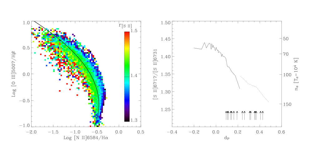
Figure 12: Left: When colour-coded according to the median value of the [S ii] $\lambda 6716$/[S ii] $\lambda 6731$ ratio, galaxies separate on the BPT diagram, even though the range of median values of this ratio is relatively small.  Right: The density sensitive [S ii] $\lambda 6716$/[S ii] $\lambda 6731$ ratio plotted vs. the parameter $d_{\rm P}$ which measures the offset perpendicular to the ridge line in Figure 5. The continuous line shows values for SDSS DR4 galaxies of class SF, while the dotted line is for galaxies classified as ‘Composite’. The values plotted are the medians in bins of 1000 galaxies each. The right-hand $y$-axis shows the conversion to the electron density $n_{\rm e}$ for a fiducial temperature $T_{\rm e}=10^{4}$ K. The arrows are plotted at the values of $d_{\rm P}$ measured for the $z>1$ star-forming galaxies in Figure 5. The [S ii] $\lambda 6716$/[S ii] $\lambda 6731$ ratio has not been measured with sufficient accuracy in any of these galaxies individually (hence the use of the arrow symbol), although from composite spectra values of $\sim 1.0-0.7$ ($n_{\rm e}\sim 1000$ cm^-3) seem typical.

3.3.3 Volume filling factor

While this parameter has potentially the most effect on the ionisation parameter (see eq. 2), it is also the one about which we know the least. In H ii regions of the Milky Way $\epsilon\sim 0.04$ (Kennicutt 1984), but we have little information on what determines this value and on how it may vary with other characteristics of the H ii regions. We have no grounds at present for assessing whether it would greater (or smaller) in actively star-forming galaxies at high redshift.

3.3.4 Density-bounded models

Equation (2) assumes that the H ii regions are ionisation bounded; relaxing this assumption can have similar effects to an increase of the ionisation parameter. Specifically, Binette, Wilson & Storchi-Bergmann (1996) considered a composite model consisting of a mixture of radiation- and matter-bounded clouds and showed that altering the proportion of the solid angle subtended by the two components, (their parameter $A_{\rm M/I}$), closely mimics changes in the ionisation parameter as far as the emission line ratios considered here are concerned. Similarly, Giammanco, Beckman, & Cedrés (2005) calculated that an escape fraction of hydrogen ionising photons $f_{\rm esc}=50$% from an H ii region would be equivalent to an increase in $U$ by one order of magnitude compared to an analogous H ii region with zero escape fraction.

Could the positions of the high redshift galaxies in the BPT diagram be a symptom that their H ii regions are ‘blistered’ and allow a higher fraction of Lyman continuum photons to escape? This possibility is difficult to assess quantitatively without more detailed modelling. From the work by Binette et al. (1996) and Giammanco et al. (2005) we estimate that considerable escape fractions, $f_{\rm esc}>10$%, would be required to explain the values of $d_{\rm P}$ exhibited by the galaxies at $z>1$ in Figure 5. Observationally, the direct measurement of $f_{\rm esc}$ has proved to be very challenging. So far, attempts to detect Lyman continuum emission in nearby galaxies have produced null results in all cases except possibly one (see Bergvall et al. 2006 and references therein; Grimes et al. 2007). The best limits at $z\simeq 1$ imply an upper limit $f_{\rm esc}<0.15$ (Siana et al. 2007), consistent with the detection of near 100% escape fraction in two out of 14 Lyman break galaxies at $z\sim 3$ and negligible values in the other 12 by Shapley et al. (2006). The difficulty in interpreting all of these measurements is that we remain essentially ignorant of what factors affect $f_{\rm esc}$; until these are understood, it is highly speculative to draw conclusions on the average escape fraction of Lyman continuum photons from galaxies on the basis of a few detections. Nevertheless, there have been claims that $f_{\rm esc}$ does evolve in the sense that it was higher at earlier times (Inoue, Iwata, & Deharveng 2006—see also Bolton et al. 2005 for less direct arguments), and therefore this could also be an important factor contributing to the offset of the high-$z$ galaxies in the BPT diagram.

3.4 Conclusions and implications

Recapitulating the main points of this section, we have found that SDSS galaxies with elevated levels of specific star formation (SFR/$M_{\star}$) tend to be offset in the BPT diagram towards higher values of the collisionally excited lines relative to the recombination lines. This is the same sense of the larger offset apparently exhibited by galaxies at $z>1$, although the numbers of such galaxies where all four nebular lines, [O iii], [N ii], H$\alpha$ and H$\beta$, have been measured so far is still very small. The response of the diagnostic emission line ratios to the excess, or deficit, of H$\alpha$ equivalent width (compared to galaxies of similar stellar mass) mirrors their response to changes in the ionisation parameter, suggesting that H ii regions of high redshift star-forming galaxies may be characterised by systematically higher values of the ionisation parameter $U$ than galaxies at the present time. Among the physical properties that may lead to higher values of $U$, we have identified high electron densities, $n_{\rm e}\sim 1000$ cm^-3, and a non-zero escape fraction of Lyman continuum photons (from nebulae which are at least partially density-bounded) as the most likely contributors on the basis of the still very limited body of available data. As the number of high-$z$ galaxies with accurate measures of the optical emission line ratios increases, it will become possible to test these ideas further with more detailed photoionisation models than warranted at present.

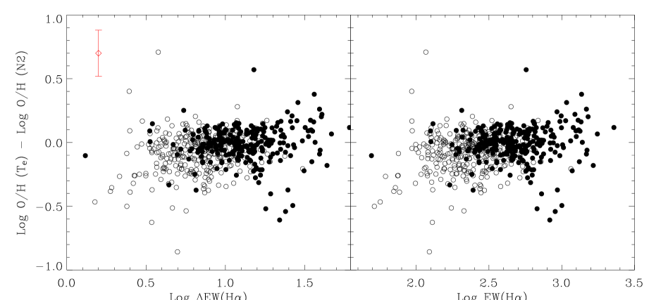
Figure 13: Left: Difference between O/H estimates from the $T_{\rm e}$ and $N2$ methods as a function of the differential H$\alpha$ equivalent width, $\Delta{\rm H}\alpha$, for 584 star-forming galaxies from the SDSS DR4. Filled dots indicate galaxies where the temperature-sensitive [O iii] $\lambda 4363$ auroral line is detected with $S/N>10$, while the open circles are for galaxies where the line is measured with an accuracy of between 10 and 20%. The error bar in the top left-hand corner indicates the median uncertainty in $\log$ [O/H ($T_{\rm e})$/O/H ($N2$)], calculated by combining in quadrature the error in O/H ($T_{\rm e})$ (mostly due to the accuracy in the measurement of the weak [O iii] $\lambda 4363$ emission line) with the $1\sigma$ scatter of 0.18 dex in the $N2$ calibration by Pettini & Pagel (2004).  Right: The oxygen abundance difference plotted as a function of the equivalent width of H$\alpha$. The only SDSS galaxies where [O iii] $\lambda 4363$ can be measured reliably are those with EW(H$\alpha)\lower 2.15277pt\hbox{$\;\buildrel>\over{\sim}\;$}100$ Å.

One of the motivations for clarifying the origin of the offset of high-$z$ galaxies in the BPT diagram was the concern that such an offset may bias metallicity measures based on the ratios of strong emission lines (the so-called strong-line methods). Among the many approaches to determining the metal content of high redshift galaxies, the calibration of the $N2$ index [$N2\equiv\log$ ([N ii] $\lambda 6583/{\rm H}\alpha)$] as a function of the oxygen abundance by Pettini & Pagel (2004) has turned out to be the most convenient to apply to high redshift star-forming galaxies for practical reasons (see Pettini 2006 for a comprehensive discussion). As we saw in Figure 8, the [N ii]/H$\alpha$ ratio, exhibits a monotonic decrease with increasing ionisation parameter at a fixed metallicity. If high redshift galaxies have systematically higher values of $U$, as argued here, what effect will that have on the calibration of O/H vs. the $N2$ index?

As a first step towards addressing this question, we compare the oxygen abundance deduced from the $N2$ index with that from the more rigorous effective temperature (or $T_{\rm e}$) method and examine whether the difference between these two values of O/H is correlated with the H$\alpha$ equivalent width offset $\Delta{\rm EW(H}\alpha$) as defined in Section 3.1. The $T_{\rm e}$ method could be applied to only 584 galaxies from SDSS DR4 (of class SF) since it relies on the detection of the weak [O iii] $\lambda 4363$ emission line. The measurement of this line, and therefore the determination of the nebular temperature, can be affected considerably from the precise placement of the underlying stellar continuum; for this reason we limited ourselves to considering galaxies where [O iii] $\lambda 4363$ is detected with a signal-to-noise ratio $S/N>5$. In deducing O/H we used the fitting functions of Izotov et al. (2006) for the $T_{\rm e}$ method and the calibration of the $N2$ index by Pettini & Pagel (2004).

As can be seen from Figure 13, the two estimators of O/H are closely related, which comes as no surprise since Pettini & Pagel calibrated the $N2$ index on $T_{\rm e}$ measurements of the oxygen abundance in nearby galaxies. What is interesting for our present enquiry is the fact that, unlike other parameters we have considered in this work, there seems to be no dependence on $\Delta{\rm EW(H}\alpha)$ of the difference in O/H between the two methods, at least for the galaxies where [O iii] $\lambda 4363$ is detected with $S/N>10$ (filled dots in Figure 13). If there are any trends with $\Delta{\rm EW(H}\alpha)$, they are masked by the larger uncertainties in the determination of the oxygen abundance with either method (indicated by the error bar in the top left-hand corner of Figure 13).

The lack of a clear trend in Figure 13 between the difference in the two measures of the oxygen abundance on the one hand, and $\Delta$EW(H$\alpha$) on the other, may be surprising at first sight. If the $N2$ index varies with $U$ at a fixed metallicity (as we saw in the lower left-hand plot in Figure 8) and if $\Delta$EW(H$\alpha$) is related to $U$, as we have argued, then might we not expect to see larger differences in $\log$ O/H($T_{\rm e})-\log$ O/H($N2$) at higher values of $\Delta$EW(H$\alpha$)? The answer to this apparent puzzle lies in the fact that the $N2$ index of Pettini & Pagel (2004) is empirically calibrated; a range of galaxies with different values of the ionisation parameter were used in the calibration, so that a given value of $N2$ does not correspond to a single value of $U$. The shallow slope of the O/H vs. $N2$ relation then results in relatively minor offsets in O/H($N2$) between galaxies with systematically different values of $U$, as already discussed by Pettini & Pagel (2004). Such offsets are apparently washed out in Figure 13 by other sources of error or intrinsic dispersion.

While the agreement between the two oxygen abundance indicators in Figure 13 is reassuring (although not unexpected, as explained), it must be borne in mind that we have been able to perform this test for only a small subset of SDSS galaxies. The galaxies where the [O iii] $\lambda 4363$ auroral line can be detected with high significance in SDSS spectra are overwhelmingly low mass, low metallicity, high $T_{\rm e}$ systems with high values of EW(H$\alpha$), as can be readily appreciated from inspection of the right-hand panel of Figure 13. Whether the agreement extends to the higher metallicities more typical of high-$z$ star-forming galaxies is a significantly more difficult question to address (e.g. Bresolin 2006, 2007 and references therein).

4 Overall Summary

In this paper we have brought together the large body of observations of local galaxies from the SDSS DR4, and state-of-the-art population synthesis models—coupled to the photoionisation code cloudy and including recent reassessments of the contributions from Wolf-Rayet stars—in order to interpret some key spectral features seen in the spectra of high redshift star-forming galaxies. Our most important findings are as follows.

1. A detectable stellar He ii $\lambda 1640$ emission line, with an equivalent width of $0.5-1.5$ Å, is expected to be present in the spectra of galaxies undergoing continuous star formation. The equivalent width of the line is stable to fluctuations in the star-formation rate, because, to a first approximation, the luminosities of the emission line and the underlying continuum are both determined by the number of massive stars.

2. In our models, the most important parameter driving EW($\lambda 1640$) is the metallicity $Z$, which affects both the fraction of W-R to O-type stars and the line luminosity in a W-R star of a given (sub-)type: at lower metallicities, fewer massive stars enter the W-R stage and the line is intrinsically weaker. Empirical data of relevance to the calibration of $L(\lambda 1640)$ vs. metallicity are still sparse, as observations of individual W-R stars have so far been largely limited to galaxies in the Local Group. However, we find an encouraging agreement between the value of EW($\lambda 1640$) calculated with our models using current estimates of the typical metallicity $Z\simeq 0.5Z_{\odot}$ of bright (${\cal R}<25.5$) UV-selected galaxies at redshifts $z=2-3$, and the value measured from the composite spectrum of hundreds of Lyman break galaxies. This result opens up the possibility of using in future the He ii $\lambda 1640$ emission line to probe the wind properties of massive stars in high redshift galaxies.

3. We have uncovered a relationship between the specific star formation rate and the position of an SDSS galaxy in the diagnostic [O iii]/H$\beta$ vs. [N ii]/H$\alpha$ nebular emission line diagram (the BPT diagram). Galaxies with excess H$\alpha$ equivalent width compared to the median for their stellar mass are displaced towards larger values of the two emission line ratios in the BPT diagram (and vice versa).

4. The responses of several emission line ratios to this parameter, which we denote as $\Delta{\rm EW(H}\alpha$), is qualitatively similar to their responses to changes in the ionisation parameter. This observation suggests that the offsets in the BPT diagram exhibited by the few star-forming galaxies at $z>1$ in which the same line ratios have been measured, may be an indication that their H ii regions are characterised by systematically larger values of the ionisation parameter $U$ than most local star-forming galaxies. Liu et al. (2008) have recently reached a similar conclusion from their analysis of a somewhat different sample of SDSS galaxies.

5. If this is the case, we identify higher electron densities and larger escape fractions of hydrogen ionising photons as two physical parameters which may be responsible for the elevated values of $U$ and, ultimately, the offsets in the BPT diagram.

6. To first order, it appears that the systematically higher values of $U$ may have only a relatively minor effect on the determination of the oxygen abundance from strong-line methods, possibly because of the larger inherent scatter in the calibrations of the most commonly used strong-line indices.

Finally, we look forward to the forthcoming availability on large telescopes of near-infrared spectrographs offering multi-object capabilities and/or wide spectral coverage; such new instrumentation will allow significant progress to be made in the investigation of the questions we have begun to explore here.

5 Acknowledgements

We gratefully acknowledge valuable discussion with Paul Crowther, Dawn Erb, Alice Shapley and Thierry Contini. JB acknowledges the receipt of FCT grant SFRH/BPD/14398/2003. An anonymous referee made a number of valuable suggestions which improved the paper.

Funding for the SDSS and SDSS-II has been provided by the Alfred P. Sloan Foundation, the Participating Institutions, the National Science Foundation, the U.S. Department of Energy, the National Aeronautics and Space Administration, the Japanese Monbukagakusho, the Max Planck Society, and the Higher Education Funding Council for England. The SDSS Web Site is http://www.sdss.org/.

The SDSS is managed by the Astrophysical Research Consortium for the Participating Institutions. The Participating Institutions are the American Museum of Natural History, Astrophysical Institute Potsdam, University of Basel, University of Cambridge, Case Western Reserve University, University of Chicago, Drexel University, Fermilab, the Institute for Advanced Study, the Japan Participation Group, Johns Hopkins University, the Joint Institute for Nuclear Astrophysics, the Kavli Institute for Particle Astrophysics and Cosmology, the Korean Scientist Group, the Chinese Academy of Sciences (LAMOST), Los Alamos National Laboratory, the Max-Planck-Institute for Astronomy (MPIA), the Max-Planck-Institute for Astrophysics (MPA), New Mexico State University, Ohio State University, University of Pittsburgh, University of Portsmouth, Princeton University, the United States Naval Observatory, and the University of Washington.

Appendix A The luminosity weighted metallicity of the composite LBG spectrum

Figure 14: Luminosity-weighted metallicity of a composite spectrum of model Lyman break galaxies where the individual have been co-added after normalising to a common mode of the signal between 1250 Å and 1500 Å, as in Shapley et al. (2003)—see text for further details. The models spectra combined to produce the composite have an average metallicity $\langle Z\rangle=0.75\,Z_{\odot}$, indicated by the dotted line.

As discussed in Section 2.2, current estimates of the nebular oxygen abundance in Lyman break galaxies are (O/H)${}_{\rm LBG}\approx 0.5\,{\rm(O/H)}_{\odot}$ (e.g. Pettini et al. 2001; Erb et al. 2006a). If this is taken to be representative of the population of LBGs brighter than $R=25.5$ (i.e. brighter than $\sim 0.5\,L^{\star}$; Reddy et al. 2007) at $z\simeq 3$, we find that there is reasonably good agreement between the value of the equivalent width of the He ii $\lambda 1640$ emission line calculated by our models and that measured from the composite spectrum of 811 LBGs constructed by Shapley et al. (2003).

In the main text of the paper we cautioned that this agreement may be somewhat fortuitous considering the significant spread in the luminosity of the He ii lines measured in stars classified as belonging to the same Wolf-Rayet spectral sub-class. Given the paucity of relevant data, the spread is still poorly determined nor are its underlying causes understood. Here we briefly consider another, more subtle, source of possible confusion in comparisons with co-added spectra of many galaxies; it is worthwhile pointing out such potential complications because the signal-to-noise ratio of single spectra is often too low for individual analysis.

In constructing their composite of 811 LBGs, Shapley et al. (2003) renormalised each spectrum to the common mode of the continuum flux between 1250 Å and 1500 Å. In principle, if there is significant range of continuum slopes among the 811 galaxies and if the slope is related to the metallicity (which seems plausible), the procedure of normalising to the mode may lead to a systematic bias in the signal near the He ii $\lambda 1640$ emission line (because galaxies of a given metallicity may contribute more than the average at a given wavelength).

We tested the magnitude of such a potential bias using a library of model spectra generated as discussed in Section 2.1. The library contains spectra produced by $\sim 10^{5}$ stochastic realisations of the population synthesis code by Bruzual & Charlot (2003). The details of this grid of models have been described by Gallazzi et al. (2005) and Salim et al. (2005, 2007); we refer the interested reader to those papers for a full discussion of how they are generated. Briefly, the star formation history is characterised by two components: an underlying continuous star formation with an exponentially declining rate determined by the parameter $\tau$ (${\rm SFR}\propto\exp[-t_{\rm sf}/\tau]$), on which random bursts can be superimposed. Dust obscuration is included so that the distribution of dust attenuation of the stellar birth clouds reproduces the distribution of H$\alpha$/H$\beta$ ratios of the star-forming galaxies in the SDSS, although for the present purposes the dust content is not very important.

From this library we select all galaxies which satisfy the LBG colour selection criteria of Steidel et al. (2003). The models span a range of metallicity $0.3<Z/Z_{\odot}<1.2$, with an average $\langle Z\rangle=3/4\,Z_{\odot}$. The model spectra were added together using the same normalisation as Shapley et al. (2003) and the luminosity-weighted metallicity was calculated at each wavelength. The results of this exercise are illustrated in Figure 14. Two cases are considered: in one case the reddening is independent of metallicity, whereas in the other $E(B-V)$ increases linearly with $Z$. The two simulated spectra are normalised so that they match at 1640 Å. Inspection of Figure 14 shows that, while there is indeed a subtle bias, in either case the effect is so small as to be inconsequential for most current applications.

References

- Adelman-McCarthy et al. (2006) Adelman-McCarthy, J. K., et al. 2006, ApJS, 162, 38
- Baldwin et al. (1981) Baldwin, J. A., Phillips, M. M., & Terlevich, R. 1981, PASP, 93, 5
- Bergvall et al. (2006) Bergvall, N., Zackrisson, E., Andersson, B.-G., Arnberg, D., Masegosa, J., & Östlin, G. 2006, A&A, 448, 513
- Binette et al. (1996) Binette, L., Wilson, A. S., & Storchi-Bergmann, T. 1996, A&A, 312, 365
- Bolton et al. (2005) Bolton, J. S., Haehnelt, M. G., Viel, M., & Springel, V. 2005, MNRAS, 357, 1178
- Brinchmann et al. (2004) Brinchmann, J., Charlot, S., White, S. D. M., Tremonti, C., Kauffmann, G., Heckman, T., & Brinkmann, J. 2004, MNRAS, 351, 1151
- Bresolin (2006) Bresolin, F. 2006, in “The Metal-Rich Universe”, eds. G. Israelian and G. Meynet (Cambridge: Cambridge University Press), in press (astro-ph/0608410).
- Bresolin (2007) Bresolin F., 2007, ApJ, 656, 186
- Bruzual & Charlot (2003) Bruzual, G., & Charlot, S. 2003, MNRAS, 344, 1000
- Chabrier (2003) Chabrier, G. 2003, PASP, 115, 763
- Chandar et al. (2004) Chandar, R., Leitherer, C., & Tremonti, C. A. 2004, ApJ, 604, 153
- Charlot & Longhetti (2001) Charlot, S., & Longhetti, M. 2001, MNRAS, 323, 887
- Crowther (2007) Crowther P. A., 2007, ARA&A, 45, 177
- Crowther & Hadfield (2006) Crowther, P. A., & Hadfield, L. J. 2006, A&A, 449, 711
- Diaz et al. (1991) Diaz, A. I., Terlevich, E., Vilchez, J. M., Pagel, B. E. J., & Edmunds, M. G. 1991, MNRAS, 253, 245
- Dopita & Sutherland (1995) Dopita, M. A., & Sutherland, R. S., 1995, ApJ, 455, 468
- Erb et al. (2006a) Erb, D. K., Shapley, A. E., Pettini, M., Steidel, C. C., Reddy, N. A., & Adelberger, K. L. 2006a, ApJ, 644, 813
- Erb et al. (2006b) Erb, D. K., Steidel, C. C., Shapley, A. E., Pettini, M., Reddy, N. A., & Adelberger, K. L. 2006b, ApJ, 646, 107
- Ferland et al. (1998) Ferland, G. J., Korista, K. T., Verner, D. A., Ferguson, J. W., Kingdon, J. B., & Verner, E. M. 1998, PASP, 110, 761
- Foellmi, Moffat, & Guerrero (2003) Foellmi C., Moffat A. F. J., Guerrero M. A., 2003, MNRAS, 338, 1025
- Gallazzi et al. (2005) Gallazzi, A., Charlot, S., Brinchmann, J., White, S. D. M., & Tremonti, C. A. 2005, MNRAS, 362, 41
- Giammanco et al. (2005) Giammanco, C., Beckman, J. E., & Cedrés, B. 2005, A&A, 438, 599
- Gonzalez-Delgado et al. (1999) González Delgado, R. M., García-Vargas, M. L., Goldader, J., Leitherer, C. & Pasquali A. 1999, ApJ, 513, 707
- Grimes et al. (2007) Grimes J. P., et al., 2007, ApJ, 668, 891
- Han, Podsiadlowski & Lynas-Gray (2007) Han, Z., Podsiadlowski, P., & Lynas-Gray, A. E. 2007, MNRAS, 380, 1098
- Heavens et al. (2004) Heavens, A., Panter, B., Jimenez, R., & Dunlop, J. 2004, Nature, 428, 625
- Inoue et al. (2006) Inoue, A. K., Iwata, I., & Deharveng, J.-M. 2006, MNRAS, 371, L1
- Izotov et al (2006) Izotov, Y. I., Stasinska, G., Meynet, G., Guseva, N. G., & Thuan, T. X. 2006, A&A, 448, 955
- Jimenez & Haiman (2006) Jimenez R., Haiman Z., 2006, Nature, 440, 501
- Kauffmann et al. (2003) Kauffmann, G., et al. 2003, MNRAS, 341, 33
- Kauffmann et al. (2006) Kauffmann, G., Heckman, T. M., De Lucia, G., Brinchmann, J., Charlot, S., Tremonti, C., White, S. D. M., & Brinkmann, J. 2006, MNRAS, 367, 1394
- Kennicutt (1984) Kennicutt, R. C., Jr. 1984, ApJ, 287, 116
- Kewley et al. (2001a) Kewley, L. J., Dopita, M. A., Sutherland, R. S., Heisler, C. A., & Trevena, J. 2001a, ApJ, 556, 121
- Kewley et al. (2001b) Kewley, L. J., Heisler, C. A., Dopita, M. A., & Lumsden, S. 2001b, ApJS, 132, 37
- Kobulnicky & Koo (2000) Kobulnicky, H. A., & Koo, D. C. 2000, ApJ, 545, 712
- Kriek et al. (2007) Kriek M., et al., 2007, ApJ, 669, 776
- Leitherer et al. (1999) Leitherer, C., et al. 1999, ApJS, 123, 3
- Leitherer et al. (2002) Leitherer, C., Li, I.-H., Calzetti, D. & Heckman, T. M. 2002, ApJS, 140, 303
- Liu et al. (2008) Liu, X., Shapley, A. E., Coil, A. L., Brinchmann, J., & Ma, C.-P., 2008, ApJ, in press
- Lowenthal et al. (1997) Lowenthal, J. D., et al. 1997, ApJ, 481, 673
- Meynet et al. (1994) Meynet, G., Maeder, A., Schaller, G., Schaerer, D., & Charbonnel, C. 1994, A&AS, 103, 97
- Meynet & Maeder (2003) Meynet, G. & Maeder, A. 2003, A&A, 404, 975
- Meynet & Maeder (2005) Meynet, G. & Maeder, A. 2005, A&A, 429, 581
- Ocvirk et al. (2006) Ocvirk, P., Pichon, C., Lançon, A., & Thiébaut, E. 2006, MNRAS, 365, 46
- Osterbrock (1989) Osterbrock, D. E. 1989, Astrophysics of gaseous nebulae and active galactic nuclei, (Suasalito, Ca: University Science Books).
- Papovich et al. (2005) Papovich, C., Dickinson, M., Giavalisco, M., Conselice, C. J., & Ferguson, H. C. 2005, ApJ, 631, 101
- Penston et al. (1990) Penston, M. V., et al. 1990, A&A, 236, 53
- Pettini (2006) Pettini, M. 2006, In “The Fabulous Destiny of Galaxies: Bridging Past and Present”, eds. V. LeBrun, A. Mazure, S. Arnouts & D. Burgarella. ISBN 2914601190. (Paris: Frontier Group), 319 (astro-ph/0603066).
- Pettini & Pagel (2004) Pettini, M. & Pagel, B. E. J. 2004, MNRAS, 348, L59
- Pettini et al. (2001) Pettini, M., Shapley, A. E., Steidel, C. C., Cuby, J.-G., Dickinson, M., Moorwood, A. F. M., Adelberger, K. L., & Giavalisco, M. 2001, ApJ, 554, 981
- Pettini et al. (2000) Pettini, M., Steidel, C. C., Adelberger, K. L., Dickinson, M., & Giavalisco, M. 2000, ApJ, 528, 96
- Reddy et al. (2006) Reddy, N. A., Steidel, C. C., Fadda, D., Yan, L., Pettini, M., Shapley, A. E., Erb, D. K., & Adelberger, K. L. 2006, ApJ, 644, 792
- Reddy et al. (2007) Reddy, N. A., Steidel, C. C., Pettini, M., Adelberger, K. L., Shapley, A. E., Erb, D. K., & Dickinson, M. 2007, ApJ, in press (astro-ph/0706.4091)
- Rix et al. (2004) Rix, S. A., Pettini, M., Leitherer, C., Bresolin, F., Kudritzki, R.-P., & Steidel, C. C. 2004, ApJ, 615, 98
- Salim et al. (2005) Salim, S., et al. 2005, ApJL, 619, L39
- Schaerer & Vacca (1998) Schaerer, D., & Vacca, W. D. 1998, ApJ, 497, 618
- Shapley et al. (2005) Shapley, A. E., Coil, A. L., Ma, C.-P., & Bundy, K. 2005, ApJ, 635, 1006
- Shapley et al. (2004) Shapley, A. E., Erb, D. K., Pettini, M., Steidel, C. C., & Adelberger, K. L. 2004, ApJ, 612, 108
- Shapley et al. (2001) Shapley, A. E., Steidel, C. C., Adelberger, K. L., Dickinson, M., Giavalisco, M., & Pettini, M. 2001, ApJ, 562, 95
- Shapley et al. (2003) Shapley, A. E., Steidel, C. C., Pettini, M., & Adelberger, K. L. 2003, ApJ, 588, 65
- Shapley et al. (2006) Shapley, A. E., Steidel, C. C., Pettini, M., Adelberger, K. L., & Erb, D. K. 2006, ApJ, 651, 688
- Siana et al. (2007) Siana B., et al., 2007, ApJ, 668, 62
- Steidel et al. (2003) Steidel, C. C., Adelberger, K. L., Shapley, A. E., Pettini, M., Dickinson, M., & Giavalisco, M. 2003, ApJ, 592, 728
- Steidel et al. (2004) Steidel, C. C., Shapley, A. E., Pettini, M., Adelberger, K. L., Erb, D. K., Reddy, N. A., & Hunt, M. P. 2004, ApJ, 604, 534
- Teplitz et al. (2000) Teplitz, H. I., et al. 2000, ApJL, 533, L65
- Tremonti et al. (2004) Tremonti, C. A., et al. 2004, ApJ, 613, 898
- van Dokkum et al (2005) van Dokkum, P. G., Kriek, M., Rodgers, B., Franx, M. & Puxley, P., 2005, ApJL, 622, L13
- Vázquez et al (2007) Vázquez, G. A., Leitherer, C., Schaerer, D., Meynet, G. & Maeder, A. 2007, ApJ, 663, 995
- Veilleux & Osterbrock (1987) Veilleux, S., & Osterbrock, D. E. 1987, ApJS, 63, 295
- Vink & de Koter (2005) Vink, J. S., & de Koter, A. 2005, A&A, 442, 587
- York et al (2000) York et al. 2000, AJ, 120, 1579