Entangled coherent states under dissipation

Abstract

We study the evolution of entangled coherent states of the two quantized electromagnetic fields under dissipation. Characteristic time scales for the decay of the negativity are found in the case of large values of the phase space distance among the states of each mode. We also study how the entanglement emerges among the reservoirs.

1 Introduction

Entanglement of two or more systems is an important concept playing a central role in quantum information science and quantum computation [1, 2]. It is an essential resource for teleportation [3], quantum key distribution [4, 5] and controlled quantum logic [6], among others. The study of entangled states of elementary quantum systems has become a fruitful field of research [1, 2, 3, 4, 5, 6, 7, 8, 9, 10, 11]. In particular, it has been paid a great attention on studying the behavior of quantum entanglement as a function of time when the system is affected by the environment [12, 13, 15, 16, 17, 18, 19, 20, 21, 22, 23].

The connection between decoherence and disentanglement has received considerable attention in the last years. Whereas decoherence of systems in contact with Markovian reservoirs decays asymptotically, entanglement may disappear suddenly. This has been recognized both in continuous variable systems [12, 13, 14] and in finite dimensional systems [15, 16, 17, 18, 19, 20]. In particular, entanglement among coherent states is a subject that has received attention by a number of authors Ref. [24, 25, 26, 27, 28, 29, 30].

The purpose of this paper is to study entanglement properties of superpositions of two-mode coherent states, in contact with a dissipative reservoir paying particular attention to the general features of the dynamics of entanglement. When the phase separation of the coherent states of each mode is large, we show, in a large variety of numerical examples, that the entanglement decays rapidly with a well defined characteristic time scale, which is much smaller than the time, $\tau$, when the entanglement completely disappears. This is in contrast to the case of two two-level systems, where the value of $\tau$ does have a physical relevance. Analytical results are also found for certain classes of states showing the same dynamical behavior. By modeling the reservoirs through a set of linear oscillators we also discuss how entanglement emerges among the reservoirs as the system looses it.

This work is organized as follows: In Sec. II we present the principal features of the entanglement dynamics under dissipation when considering as the initial state a general superposition of two coherent states for each mode. In Sec. III we study particular situations where we may easily describe analytically the time evolution of the negativity and the conditions for complete disentanglement. In Sec. IV we consider explicitly the reservoir degrees of freedom, in order to describe how the entanglement emerges into the two reservoirs. Finally, in Sec. V we present our concluding remarks.

2 Disentanglement dynamics

Consider the dynamics of two dissipative quantum modes, each affected by its own environment. Such a situation can be conveniently described at zero temperature by the master equation

$$\hat{\dot{\rho}}=\frac{\Gamma_{a}}{2}\left(2\hat{a}\hat{\rho}\hat{a}^{\dagger}-\hat{a}^{\dagger}\hat{a}\hat{\rho}-\hat{\rho}\hat{a}^{\dagger}\hat{a}\right)+\frac{\Gamma_{b}}{2}\left(2\hat{b}\hat{\rho}\hat{b}^{\dagger}-\hat{b}^{\dagger}\hat{b}\hat{\rho}-\hat{\rho}\hat{b}^{\dagger}\hat{b}\right),$$ (1)

where $\hat{a},\hat{a}^{\dagger}$ and $\hat{b},\hat{b}^{\dagger}$ are the annihilation and creation operators of the two modes.

Consider the class of initially entangled pure states of the form

$$\left|\Psi\right\rangle=\sum_{i,k=1,2}c_{i}^{k}\left|\alpha_{i}\right\rangle\left|\beta_{k}\right\rangle,$$ (2)

where $\left|\alpha_{{}_{1}}\right\rangle$ and $\left|\alpha_{{}_{2}}\right\rangle$ ($\left|\beta_{{}_{1}}\right\rangle$ and $\left|\beta_{{}_{2}}\right\rangle$ ) are coherent states associated with mode $a$ (mode $b$) and $c_{i}^{k}$ ($i,k=1,2$), are complex constants. An important feature of the solution of Eq. (1) for $\hat{\rho}(t)$ is that, for each $t$ it can be written only in terms of the operators $|\alpha_{i}(t),\beta_{m}(t)\rangle$ $\langle\alpha_{j}(t),\beta_{n}(t)|.$ In fact, it can be shown that this solution is given by

$$\hat{\rho}(t)=\sum_{i,j,m,n=1,2}C_{i,j}^{m,n}(t)|\alpha_{i}(t)\beta_{m}(t)\rangle\langle\alpha_{j}(t)\beta_{n}(t)|,$$ (3)

where $\alpha_{i}(t)=\alpha_{i}e^{-\Gamma_{a}t/2},\,\beta_{i}(t)=\beta_{i}e^{-\Gamma_{b}t/2},\ i=1,2,$ and

$$\begin{array}[]{l}C_{i,j}^{m,n}(t)=c_{i}^{m}(c_{j}^{n})^{\ast}\exp{\{-(1-e^{-\Gamma_{a}t})(|\alpha_{i}-\alpha_{j}|^{2}}+2i\mathrm{{Im}(\alpha_{i}\alpha_{j}^{\ast}))/2\}\times}\\ \exp{\{-(1-e^{-\Gamma_{b}t})(|\beta_{m}-\beta_{n}|^{2}}+2i\mathrm{{Im}({\beta_{m}\beta}_{n}^{\ast}))/2\}}.\end{array}$$ (4)

The state above could be conveniently written in an orthogonal basis for each time $t.$ For example, we could use the basis

$$|\xi_{\pm}(t)\rangle = N_{\xi_{\pm}}\bigg{(}|\xi_{1}(t)\rangle\pm\frac{\langle\xi_{2}(t)|\xi_{1}(t)\rangle}{|\langle\xi_{2}(t)|\xi_{1}(t)\rangle|}|\xi_{2}(t)\rangle\bigg{)},$$ (5)

with $N_{\xi\pm}=1/\sqrt{2(1\pm|\langle\xi_{2}(t)|\xi_{1}(t)\rangle|)}$ and $\xi=\alpha,\beta$.

Although our system is a continuous one, it evolves in such way that at any time t it can be described in the time dependent subspace spanned by the vectors $\left|\alpha_{\pm}(t)\right\rangle\otimes\left|\beta_{\pm}(t)\right\rangle$. In this basis, we are allowed to treat the whole system as an effective two-qubit system [31] so that we can study entanglement properties through the concurrence [32]

$$C(t)={\rm{max}}\{0,(\lambda_{1}-\lambda_{2}-\lambda_{3}-\lambda_{4})\},$$ (6)

where $\lambda_{i}(t),i=1,2,3,4$ are the square root of eigenvalues, in decreasing order, of the matrix $M(t)=\rho(t)\sigma_{1y}\otimes\sigma_{2y}\rho(t)^{*}\sigma_{1y}\otimes\sigma_{2y},$ with all matrices been written in the time dependent 4-dimensional basis [Eq. (5)].

The coherence of a superposition of a pair of coherent states decays for short times with a time scale depending on the distance between the superposed states and almost disappears much before the characteristic time for energy dissipation. The problem we want to address here is how entanglement is lost for a pair of entangled coherent states and how it depends on the initial conditions. For any state of the form of Eq. (3) there is no simple analytical expression to describe how the entanglement evolves. In this section we take a numerical approach to get some insight in understanding the evolution of entanglement as a function of distances between the superposed states.

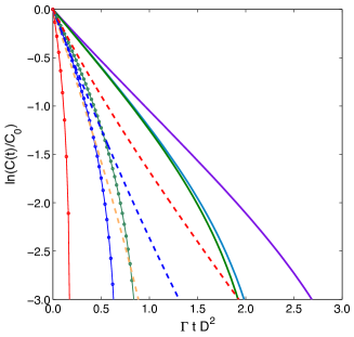
Figure 1: $\ln C(t)/C(0)$ as a function of $t/\tau,$ for $D^{2}=0.75$ (line and circles), $D^{2}=2$ ( dashed line) and $D^{2}=5$ (solid line ). For each value of $D^{2}$, three sets of coefficients $c_{i}^{k}$ that define the initial state (2) were chosen at random. $\Gamma_{a}=\Gamma_{b}=\Gamma$

For short times compared with $1/\Gamma_{a}(1/\Gamma_{b})$ the matrix elements $C_{i,j}^{n,n},i\neq j,$ ( $C_{i,i}^{m,n},m\neq n,$ ) decay exponentially with a time constant $\tau_{a}=\left[(\Gamma_{a}|\alpha_{1}-\alpha_{2}|^{2})/2\right]^{-1}$ ( $\tau_{b}=\left[(\Gamma_{b}|\beta_{1}-\beta_{2}|^{2})/2\right]^{-1}$ ). $\tau_{a}$ ($\tau_{b}$) are time scales associated to the loss of coherence among the states $|\alpha_{1}\rangle$ ($|\beta_{1}\rangle$) and $|\alpha_{2}\rangle$($|\beta_{2}\rangle$ of mode $a$ $(b).$ Entanglement, as measured by the concurrence, Eq.6, is a sum of non linear functions of the matrix elements $C_{i,j}^{m,n}(t),$ and, depending on the initial conditions, may even vanishes at finite times although the matrix elements $C_{i,j}^{m,n}(t),$ only vanish at infinity. On physical grounds, we expect that entanglement evolution will depend mostly on the matrix elements $C_{i,j}^{m,n}(t)$ with $i\neq j,m\neq n.$ Therefore for values of $D^{2}=(|\alpha_{1}-\alpha_{2}|^{2}+|\beta_{1}-\beta_{2}|^{2})/2\gg 1,$ and for times shorter than $1/\Gamma_{a}$ and $1/\Gamma_{b}$ the concurrence should initially drop exponentially in a characteristic time $\tau=1/[(\Gamma_{a}|\alpha_{1}-\alpha_{2}|^{2}+\Gamma_{b}|\beta_{1}-\beta_{2}|^{2})/2].$ We show examples of this behavior by plotting, in Fig. 1, $\ln C(t)/C(0)$ versus $t/\tau$ for $\Gamma_{a}=\Gamma_{b}$, for fixed values of $D^{2}=(|\alpha_{1}-\alpha_{2}|^{2}+|\beta_{1}-\beta_{2}|^{2})/2$ and for values of the constants $c_{i}^{k}$ chosen at random. The curves show evidence that the entanglement initially does follow a single exponential behavior. After a while some of the curves drop more rapidly showing evidence of a non asymptotic decay of the concurrence, suggesting that finite time complete disentanglement is present for a variety of states. In the next section we study special cases for which one may obtain simple analytical results for the concurrence.

3 Special cases

In this section we consider certain classes of states where we are able to find simple analytical results for the concurrence, showing explicitly the behavior of disentanglement suggested in the last section. In all cases we take, for simplicity, $\Gamma_{a}=\Gamma_{b}=\Gamma$ and the amplitudes $\alpha_{1}(\beta_{1})$ and $\alpha_{2}(\beta_{2})$ of the states in Eq. (2) having the same phase. The density matrix in Eq. (3) can then be written at each time $t$ in the orthogonal basis defined by

$$\mid\pm,t\rangle_{a} = N_{a\pm}(t)(\mid\alpha_{1}({t})\rangle\pm\mid\alpha_{2}({t})\rangle)$$

$$\mid\pm,t\rangle_{b} = N_{b\pm}(t)(\mid\beta_{1}({t})\rangle\pm\mid\beta_{2}({t})\rangle),$$ (7)

where

$$N_{a\pm}(t) = 1/\sqrt{2(1\pm e^{-\frac{1}{2}(|\alpha_{1}-\alpha_{2}|^{2})e^{-\Gamma t}})}$$

$$N_{b\pm}(t) = 1/\sqrt{2(1\pm e^{-\frac{1}{2}(|\beta_{1}-\beta_{2}|^{2})e^{-\Gamma t}})}$$

We also use, from now on the negativity, defined as smallest eigenvalue of the partial transposition matrix $\rho^{T_{A}}$ [33, 34], as a measure of entanglement.

As a first example we consider the state

$$|\Psi\rangle=\frac{1}{2}(|\alpha_{1}\beta_{1}\rangle+|\alpha_{1}\beta_{2}\rangle+|\alpha_{2}\beta_{1}\rangle-|\alpha_{2}\beta_{2}\rangle),$$ (9)

which is a very high entangled state whenever $d_{\alpha}^{2}=|\alpha_{1}-\alpha_{2}|^{2}/2\gg 1$ and $d_{\beta}^{2}=|\beta_{1}-\beta_{2}|^{2}/2\gg 1$. Within these conditions we obtain a simple form for the negativity:

$$\lambda_{-}=(1-e^{(e^{-\Gamma_{a}t}-1)d_{\alpha}^{2}}-e^{(e^{-\Gamma_{b}t}-1)d_{\beta}^{2}}-e^{(e^{-\Gamma_{a}t}-1)d_{\alpha}^{2}}e^{(e^{-\Gamma_{b}t}-1)d_{\beta}^{2}})/4,$$ (10)

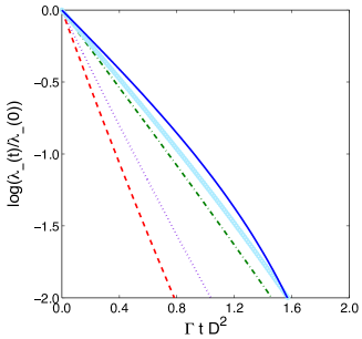
Figure 2: $\ln\lambda(t)/\lambda(0)$ as a function of the renormalized time $t\left[(\Gamma_{a}|\alpha_{1}-\alpha_{2}|^{2}+\Gamma_{b}|\beta_{1}-\beta_{2}|^{2})/2\right],$ for the state given by Eq. 9. $D^{2}=0.5$ (dashed line), $D^{2}=0.75$ (dotted line), $D^{2}=1.5$ (dot-dashed line), $D^{2}=2$ (circles), $D^{2}=5$ (solid line). $\Gamma_{a}=\Gamma_{b}=\Gamma$

so that entanglement decays with a superposition of exponentials within a characteristic time $1/\left[\Gamma(d_{\alpha}^{2}+d_{\beta}^{2})\right]$ as suggested in section II. Numerical results for the negativity are shown in Fig. 2, for $\Gamma_{a}=\Gamma_{b}=\Gamma$ and $D^{2}=(d_{\alpha}^{2}+d_{\beta}^{2})/2$ equals to $0.5,0.75,1.5,2$ and $5$. As we observe in the figure, $\ln\lambda_{-}(t)/\lambda_{-}(0)$ as a function of $\Gamma D^{2}t$ has a slope close to $-1,$ even for $D^{2}$ as small as 2.

Consider now that the system is initially prepared in entangled states of the form

$$\left|\Psi\right\rangle=c_{+,+}\left|+,0\right\rangle_{a}\left|+,0\right\rangle_{b}+c_{-,-}\left|-,0\right\rangle_{a}\left|-,0\right\rangle_{b},$$ (11)

where, without loss of generality, $c_{+,+}$ and $c_{-,-}$ are taken as real and positive constants. The density matrix written in the basis $\{\mid\pm\pm,t\rangle:=\mid\pm,t\rangle_{a}\otimes\mid\pm,t\rangle_{b}\}$ has the form of an $X-{\rm matrix}$ as previously considered for studying finite-time disentanglement [18, 19, 20]. In such case it can be shown that the concurrence is related to the negativity, $\lambda_{-},$ by the expression $C(t)=\textrm{max}\{0,-2\lambda_{-}\}.$ For simplicity, let us assume equal distances for each mode, $\left|\alpha_{1}-\alpha_{2}\right|=|\beta_{1}-\beta_{2}|$. The negativity can then be easily calculated and it is given by

$$\lambda_{-}=\left[1-e^{-D^{2}e^{-\Gamma t}}\right]\left[A_{2}^{2}-A_{1}^{2}e^{-D^{2}(1-e^{-\Gamma t})}\right],$$ (12)

with $A_{1}=c_{+,+}N_{a+}(0)N_{b+}(0)+c_{-,-}N_{a-}(0)N_{b-}(0)$ and $A_{2}=c_{+,+}N_{a+}(0)N_{b+}(0)-c_{--}N_{a-}(0)N_{b-}(0)$.

Complete disentanglement occurs when the eigenvalue $\lambda_{-}$ becomes positive. From the expression above it is easy to see that this happens in a time $t_{\rm{d}}^{(1)}$ given by:

$$t_{\rm{d}}^{(1)}=-\frac{1}{\Gamma}\ln\left(1+\frac{2}{D^{2}}\ln\left(\frac{\left|A_{2}\right|}{\left|A_{1}\right|}\right)\right).$$ (13)

The condition for having finite disentanglement time is that $\exp(-D^{2}/2)<\left|A_{2}\right|/\left|A_{1}\right|,$ which can be satisfied in two different cases. Firstly for $c_{-,-}/f>c_{+,+}$, with $f=(1-e^{-D^{2}/2})/(1+e^{-D^{2}/2})$ for which there is always a finite disentanglement time $t_{\rm{d}}^{(1)}$ if $c_{-,-}>c_{+,+}$ . Secondly when $c_{+,+}>c_{-,-}/f$, where there is $t_{\rm{d}}^{(1)}$ finite only if $c_{-,-}<c_{+,+}f^{2}$.

For large distances, $D\gg 1$, we see from Eq. (12) that the concurrence drops exponentially with a characteristic time $(D^{2}\Gamma)^{-1},$ which is much shorter than the dissipation time $\Gamma^{-1},$ in agreement with the results suggested in section II.

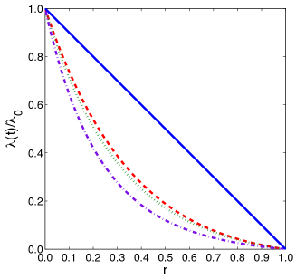
Figure 3: Ratio of the negativity at time $t$ and at the initial time as a function of the normalized time $r=t/t_{\rm{d}}^{(1)}$, for fixed $|c_{--}/c_{++}|=\sqrt{2}$ and distances $D^{2}=0.5$ (dashed line), $D^{2}=2$ (dotted line) and $D^{2}=7.5$ (dot-dashed line). It is also shown, for comparison, the line $1-r$.

Although the loss of entanglement may happen at a finite time $t_{\rm{d}}^{(1)}$, the concurrence, for $D>1,$ is already small at a much earlier time. A similar result was found in Ref. [35] when studying GHZ $N$ qubits states under different independent reservoirs. Consider, for example, the expression (12) for the case of the initial state given by Eq. (11). For $D^{2}\gg 1,$ $\Gamma t_{\rm{d}}^{(1)}\ll 1$ we can easily show that the negativity drops significantly to low values much before the time $t_{d}$ when it completely disappears, independently of the values of $c_{++},c_{--}$ and $D.$ In Fig. 3 we show the behavior of the negativity for a fixed value of the ratio $c_{++}/c_{--}$ and for several values of $D^{2},$ as a function of the normalized time $r=t/t_{\rm{d}}^{(1)}$. From that figure we see that the negativity drops to very low values in a time less than half the complete disentanglement time $t_{d}.$

For small distances, $D\ll 1,$ Eq. (12) can be approximated to

$$\lambda_{-}\simeq c_{--}^{2}e^{-\Gamma t}\left[1-\frac{c_{++}}{c_{--}}-e^{-\Gamma t}\right].$$ (14)

The interesting about this regime is that clearly shows two different scales of disentanglement depending on the values of $c_{++}$ and $c_{--}$. In particular, for an initial maximally entangled state, that is, $c_{++}=c_{--}=1/\sqrt{2}$, $\lambda_{-}\simeq-(1/2)\exp{(-2\Gamma t})$ the entanglement decays asymptotically with a rate $2\Gamma$. For $c_{-,-}>c_{+,+}$ entanglement vanish for time $t_{d}=-\Gamma^{-1}\ln(1-c_{+,+}/c_{-,-})$. For $c_{-,-}<c_{+,+}$ entanglement decays always asymptotically. So that this case behaves in a similar way to the two-qubit case in [20].

Other situation of interest is the class of initial states having the form:

$$\left|\Phi\right\rangle=c_{+,-}|+,0\rangle_{a}\left|-,0\right\rangle_{b}+c_{-,+}\left|-,0\right\rangle_{a}\left|+,0\right\rangle_{b},$$ (15)

where $c_{+,-}$, $c_{-,+}$ are taking as real constants. The dynamics of this state leads also to an X density matrix. In a similar way as for the previous case, we found that the time for disentanglement is given by:

$$t_{\rm{d}}^{(2)}=-\frac{1}{\Gamma}\ln\left(1+\frac{2}{D^{2}}\ln\left|\frac{(c_{+,-}-c_{-,+})}{(c_{+,-}+c_{-,+})}\right|\right).$$ (16)

The only condition required for having $t_{\rm{d}}^{(2)}$ finite is that:

$$\exp(-\frac{1}{2}D^{2})<\left|(c_{+,-}-c_{-,+})/(c_{+,-}+c_{-,+})\right|.$$ (17)

4 Birth of entanglement among the reservoirs

In the above sections, we have studied disentanglement dynamics for some special cases of entangled coherent states, paying attention only to the system of the modes $a$ and $b$. However, when including degrees of freedom of both reservoirs, a deeper understanding of entanglement dynamics can be obtained. This can be carried out by describing the system-reservoir dynamics per each mode with a Hamiltonian of the form [37]

$$H=\hbar\omega a^{\dagger}a+\hbar\sum_{k=1}^{N}\omega_{k}c^{\dagger}_{k}c_{k}+\hbar\sum_{k=1}^{N}g_{k}(ac^{\dagger}_{k}+c_{k}a^{\dagger}).$$ (18)

In such case, it is not difficult to show that when the mode $a$ is initially in a coherent state and the reservoir is in the collective vacuum state $|\bar{0}\rangle_{r}=\prod^{N}_{k=1}|0_{k}\rangle_{r}$, the mode $a$ and its reservoir evolve into a product of coherent states of the form $\mid\alpha_{t}\rangle|{\bar{\alpha}_{t}}\rangle_{r}=\mid\alpha F(t)\rangle\prod^{N}_{k=1}|f_{k}(t)\alpha\rangle_{r}.$ In the Born-Markov approximation $F(t)=e^{-\Gamma_{a}t/2}$ and $\sum_{k}f_{k}(t)^{2}=1-e^{-\Gamma_{a}t}.$

To illustrate how entanglement emerges into the reservoirs, let us consider the initial state of Eq. (11), but now including the states for both reservoirs

$$\left|\Psi\right\rangle=\big{(}c_{+,+}\left|+,0\right\rangle_{a}\left|+,0\right\rangle_{b}+c_{-,-}\left|-,0\right\rangle_{a}\left|-,0\right\rangle_{b}\big{)}|\bar{0}\rangle_{r_{a}}|\bar{0}\rangle_{r_{b}},$$ (19)

where $c_{+,+}$ and $c_{-,-}$ are real and positive constants. Note that $a(b)$ and $r_{a(b)}$ stand for mode $a(b)$ and reservoir associated to mode $a(b)$, respectively. Since the evolution of each mode and its reservoir may be treated independently, the complete density matrix at time $t$ can be obtained through the evolution of the states $|\pm,0\rangle_{a}|\bar{0}\rangle_{r_{a}}=N_{a\pm}(0)\big{(}|\alpha\rangle\pm|-\alpha\rangle\big{)}|\bar{0}\rangle_{r_{a}}$ and $|\pm,0\rangle_{b}|\bar{0}\rangle_{r_{b}}=N_{b\pm}(0)\big{(}|\beta\rangle\pm|-\beta\rangle\big{)}|\bar{0}\rangle_{r_{b}}.$

Let $c$ and $r_{c}$ stand for either mode $a$ or $b$ and for their own reservoirs. It is possible to show that the initial states $|+,0\rangle_{c}|\bar{0}\rangle_{r_{c}}$ and $|-,0\rangle_{c}|\bar{0}\rangle_{r_{c}}$ evolve at the time $t$ to the states

$$|\phi_{+,t}\rangle_{rc} = \frac{N_{c+}(0)B_{c+}(t)}{2N_{c+}(t)}|+,t\rangle_{c}|E_{+,t}\rangle_{r_{c}}+\frac{N_{c+}(0)B_{c-}(t)}{2N_{c-}(t)}|-,t\rangle_{c}|E_{-,t}\rangle_{r_{c}}$$

$$|\phi_{-,t}\rangle_{rc} = \frac{N_{c-}(0)B_{c-}(t)}{2N_{c+}(t)}|+,t\rangle_{c}|E_{-,t}\rangle_{r_{c}}+\frac{N_{c-}(0)B_{c+}(t)}{2N_{c-}(t)}|-,t\rangle_{c}|E_{+,t}\rangle_{r_{c}}\,,$$

respectively. The states $|E_{\pm,t}\rangle_{r_{c}}$ in the equations above are defined as $|E_{\pm,t}\rangle_{r_{a}}=\big{(}|\bar{{\bf\alpha}_{t}}\rangle_{r_{a}}\pm|-\bar{{\bf\alpha}_{t}}\rangle_{r_{a}}\big{)}/B_{a\pm}(t)$ and $|E_{\pm,t}\rangle_{r_{b}}=\big{(}|\bar{{\bf\beta}_{t}}\rangle_{r_{a}}\pm|-\bar{{\bf\beta}_{t}}\rangle_{r_{a}}\big{)}/B_{b\pm}(t)$ and form a two-dimensional orthogonal basis for each reservoir, and normalization terms read

$$B_{a\pm}(t) = \sqrt{2(1\pm e^{-{2}|\alpha|^{2}(1-e^{-\Gamma_{a}t})})}\,,$$

$$B_{b\pm}(t) = \sqrt{2(1\pm e^{-{2}|\beta|^{2}(1-e^{-\Gamma_{b}t})})}.$$ (21)

Let us now study the joint evolution of the two modes coupled to their reservoirs. In the above description, the initial state (19) evolves to

$$|\Psi\rangle_{t}=c_{++}|\phi_{+,t}\rangle_{ar_{a}}|\phi_{+,t}\rangle_{br_{b}}+c_{--}|\phi_{-,t}\rangle_{ar_{a}}|\phi_{-,t}\rangle_{br_{b}}.$$ (22)

This is a pure state representing the whole system. As $t$ increases, there is a transfer of the correlations of the system, both classical and quantum, to the reservoirs. Notice that there is no memory effects involved in this transfer. Information about the reservoir-reservoir dynamics are obtained by tracing out cavities degrees of freedom, as well as the cavity modes evolution are obtained by tracing out the states of the reservoirs.

As before, let us consider equal distances for each mode, $D^{2}=|\alpha_{1}-\alpha_{2}|^{2}=|\beta_{1}-\beta_{2}|^{2}$. The dynamics given by Eq. (22) leads us to an $X-{\rm matrix}$ for the reservoir-reservoir subsystem, which is complementary to the density matrix of the subsystem of the two modes $a$ and $b$ [37]. As a consequence, we can study entanglement dynamics associated to external degrees of freedom.

When studying entanglement through the partial transposition matrix, we obtain a complementary result of (12) giving us information about the birth of entanglement in the reservoir-reservoir subsystem. In this case, we obtain the following negative eigenvalue

$$\lambda_{-}=\left[1-e^{-D^{2}(1-e^{-\Gamma t})}\right]\left[A_{2}^{2}-A_{1}^{2}e^{-D^{2}e^{-\Gamma t}}\right],$$ (23)

from which we can derive the time for birth of entanglement in reservoirs, that is

$$t_{b}=-\frac{1}{\Gamma}\ln\bigg{(}\frac{2}{D^{2}}\ln\bigg{(}\frac{|A_{1}|}{|A_{2}|}\bigg{)}\bigg{)}.$$ (24)

Note that Eq. (23) can be obtained from Eq. (12) by exchanging the time-dependent functions, $e^{-\Gamma t}$ and $1-e^{-\Gamma t}$. Also

$$e^{-\Gamma t_{d}}+e^{-\Gamma t_{b}}=1$$ (25)

This result immediately shows that if the entanglement among the two modes persists all the time, the entanglement among the reservoirs starts growing at $t=0.$ Eqs. (13) and (24) shows that in this case the entanglement among the reservoirs never dies and its negativity reaches at infinity the initial value of the negativity among the two modes $a$ and $b.$ Eq. (25), together with Eqs. (13) and (24) also shows that the time when entanglement starts among the two reservoirs can be either smaller, greater or equal to the time when entanglement among the two modes completely disappears. This result is analogous to the one obtained in Ref. [37].

Figure 4 shows the entanglement evolution when $t_{b}>t_{d}$, considering two distances in phase space $D^{2}=0.4$ (Fig. 4(a)) and $D^{2}=16$ (Fig. 4(b)). Here there is a time window where no entanglement exist either among the two modes or among the two reservoirs. However, we observe that entanglement does exist in others bipartite partitions of the whole system, since each mode entangles with the reservoir of the other mode. When plotting the concurrences $\mathcal{C}_{ab}$, $\mathcal{C}_{r_{a}r_{b}}$, $\mathcal{C}_{ar_{a}}$ and $\mathcal{C}_{ar_{b}}$, we notice that in the region where there is no entanglement either among the modes $a$ and $b$ or among the two reservoirs, that is, $\mathcal{C}_{ab}=\mathcal{C}_{r_{a}r_{b}}=0$, entanglement between a mode and its corresponding reservoir reaches its maximum value. Although this behavior is presented in both cases, the correlations are sensitive to any change of parameter $D^{2}$, as shown in Fig. 4(b) where the concurrence between mode $a$ and reservoir $r_{b}$ is very small. Moreover for small distances ($D^{2}=|2\alpha|^{2}$), which also correspond to a small average number of photons, we reproduce the entanglement dynamics associated to the two-qubit case studied in Ref. [37]. Note that since we are considering equal distances and decay rates, both mode-reservoir subsystems evolves identically implying that the concurrences $\mathcal{C}_{ar_{a}}=\mathcal{C}_{br_{b}}$ and $\mathcal{C}_{ar_{b}}=\mathcal{C}_{br_{a}}$.

A particular result happens when $|A_{1}/A_{2}|=e^{D^{2}/4},$ that is $c_{+,+}/c_{-,-}=(1+e^{-D^{2}/2})/(1-e^{-D^{2}/4})^{2}$. In this case, the times when the modes completely disentangles and the time when the reservoirs starts to be entangled are equal and occurs at $t_{b}=t_{d}=\ln(2)/\Gamma,$ a result which in independent of the distances in phase space for both modes.

5 Conclusion

In conclusion, we have studied the evolution, under dissipation, of the entanglement among two modes of the electromagnetic field for certain class of initially entangled coherent states. At zero temperature, the density matrix can always be written, for each $t,$ in a finite orthogonal basis, which allow us to describe the entanglement evolution as that happening in a discrete system. Asymptotic entanglement decay as well as finite time disentanglement arises depending on the initial conditions for the bipartite system and on the distances in phase space among the components of each mode. Typically, the robustness of entanglement decays in a time scale proportional to $2/(\Gamma_{a}|\alpha_{1}-\alpha_{2}|^{2}+\Gamma_{b}|\beta_{1}-\beta_{2}|^{2})$, the inverse of a weighted average of the distances in phase space for each mode, whenever these distances are much greater than one. Both numerical and analytical results are presented.

We have also presented an investigation concerning the entanglement generation among the reservoirs. By modeling the reservoir and its interaction with the system, it is possible to study death of entanglement among both modes of the field and the birth of entanglement in reservoir-reservoir subsystem, respectively. In addition to the dependence on initial amplitudes, the characteristic times for death and birth of entanglement depends on the distances among coherent states. An interesting result shows that for specific conditions in the initial amplitudes for a given distance among coherent states, both birth and death of entanglement at finite times occur simultaneously at a time which does not depend on the distances of each mode.

Acknowledgements

F.L. acknowledges Fondecyt 3085030, G.R. acknowledges Juan de la Cierva Program, C.E.L. acknowledges Fondecyt 11070244 and PBCT-CONICYT PSD54, J.C.R. acknowledges Fondecyt 1070157. N.Z. acknowledges the support from CNPq and FAPERJ. C.E.L. and J.C.R. acknowledge support from Financiamiento Basal para Centros Cientícos y Tecnológicos de Excelencia.

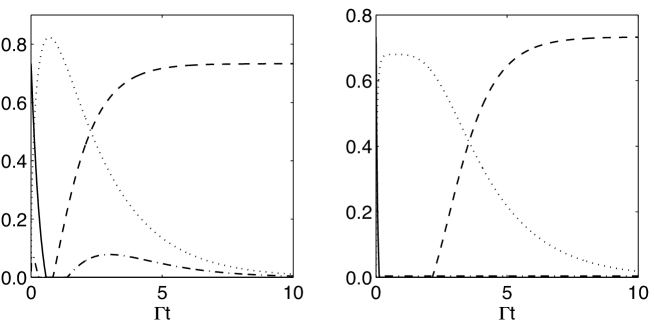
Figure 4: Evolution of concurrence for different bipartite partitions. $\mathcal{C}_{c_{a}c_{b}}$ (solid line), $\mathcal{C}_{r_{a}r_{b}}$ (dashed line), $\mathcal{C}_{c_{a}r_{a}}$ (dotted line), and $\mathcal{C}_{c_{a}r_{b}}$ (dot-dashed line). (a) considering $D^{2}=0.4$ and (b) for $D^{2}=16$. In both simulations we considered equal decay rates $\Gamma_{a}=\Gamma_{b}=\Gamma$, and amplitudes are $c_{+,+}=0.4$, $c_{-,-}=\sqrt{1-c_{+,+}^{2}}$.

References

• [1] M.A. Nielsen and I.L. Chuang, Quantum Computation and Quantum Information (Cambridge Univ. Press., Cambridge, 2000).
• [2] A. Ekert and R. Jozsa, Rev. Mod. Phys. 68, 733 (1996).
• [3] C. H. Bennett, G. Brassard, C. Crépeau, R. Jozsa, A. Peres, and W. K. Wootters, Phys. Rev. Lett. 70, 1895 (1993).
• [4] A. K. Ekert, Phys. Rev. Lett. 67, 661 (1991).
• [5] N. Gisin, G. Ribordy, W. Tittel, and H. Zbinden, Rev. Mod. Phys. 74, 145 (2002).
• [6] E. Knill, R. Laflamme, and G. J. Milburn, Nature 409, 46 (2001).
• [7] W. Tittel and G. Weihs, Quantum Inf. Comput. 2, 3 (2001)
• [8] D. Leibfried, R. Blatt, C. Monroe, and D. Wineland, Rev. Mod. Phys. 75, 281 (2003).
• [9] L. M. K. Vandersypen and I. L. Chuang, Rev. Mod. Phys. 76, 1037 (2004).
• [10] J. M. Raimond, M. Brune, and S. Haroche, Rev. Mod. Phys. 73, 565 (2001).
• [11] R. Hanson, L. P. Kouwenhoven, J. R. Petta, S. Tarucha,and L. M. K. Vandersypen, Rev. Mod. Phys. 79, 1217 (2007).
• [12] L.-M. Duan, G. Giedke, J. I. Cirac, and P. Zoller, Phys. Rev. Lett. 84, 2722 (2000)
• [13] J. S. Prauzner-Bechcicki, J. Phys. A: Math. Gen. 37 (2004) L173-L181.
• [14] R. Olkiewicz and M. Żaba, J. Phys. B: At. Mod. Opt. Phys. 42 (2009) 205504.
• [15] K. Życzkowski, P. Horodecki, M. Horodecki, and R. Horodecki, Phys. Rev. A 65, 012101 (2001).
• [16] L. Diósi, Lect. Notes Phys. 622, 157-163 (2003).
• [17] P. J. Dodd and J. J. Halliwell, Phys. Rev. A, 69, 052105 (2004).
• [18] T. Yu and J. H. Eberly, Phys. Rev. Lett. 93, 140404 (2004); idem 97, 140403 (2006).
• [19] M. Yönaç, T. Yu and J. H. Eberly, J. Phys. B 39, S621 (2006).
• [20] M. F. Santos, P. Milman, L. Davidovich, and N. Zagury, Phys. Rev. A. 73, 040305(R), 2006.
• [21] A. Jamróz, J. Phys. A 39, 7727 (2006), Z. Ficek and R. Tanaś, Phys. Rev. A 74, 024304 (2006), A. Vaglica and G. Vetri, arXiv:quant-ph/0703241; Mahmoud Abdel-Aty and H. Moya-Cessa, arXiv:quant-ph/0703077; H. T. Cui, K. Li, and X. X. Yi, arXiv:quant-ph/0612145; Mahmoud Abdel-Aty, arXiv:quant-ph/0610186.
• [22] M. P. Almeida, et al., Sience 316, 579 (2007).
• [23] J. Laurat, K. S. Choi, H. Deng, C.W. Chou, and H. J. Kimble, Phys. Rev. Lett. 99, 180504 (2007).
• [24] B. C. Sanders, Phys. Rev. A 45, 6811 (1992).
• [25] R. Filip, J. Rehácek, and M. Dusek, J. Opt B: Quantum-semiclassical Opt. 3, 341 (2001).
• [26] S. J. van Enk and O. Hirota, Phys. Rev. A 64, 022313 (2001).
• [27] H. Jeong, M. S. Kim, and J. Lee, Phys. Rev. A 64, 052308 (2001).
• [28] X. Wang, J. Phys. A: Math. Gen. 35, 165 (2002).
• [29] S. J. van Enk, Phys. Rev. Lett. 91, 017902 (2003).
• [30] S. J. van Enk, Phys. Rev. A 72, 022308 (2005).
• [31] A two-qubit treatment of such a systems has also been considered in [27].
• [32] S. Hill and W. K. Wootters, Phys. Rev. Lett. 78, 5022 (1997); W. K. Wootters, Phys. Rev. Lett. 80, 2245 (1998).
• [33] A. Peres, Phys. Rev. Lett. 77, 1413 (1996).
• [34] M. Horodecki, P. Horodecki, R. Horodecki, Phys. Lett. A 223, 1 (1996).
• [35] L. Aolita, R. Chaves, D. Cavalcanti, A. Acín, and L. Davidovich, Phys. Rev. Lett. 100 080501 (2008).
• [36] K. Chen, S. Albeverio, S. Fei, Phys. Rev. Lett. 95, 210501 (2005).
• [37] C.E. López, G. Romero, F. Lastra, E. Solano and J. C. Retamal, Phys. Rev. Lett. 101, 080503 (2008).
Refer to caption