Statistical Analysis of Crossed Undulator for Polarization Control in a SASE FEL

Abstract

There is a growing interest in producing intense, coherent x-ray radiation with an adjustable and arbitrary polarization state. In this paper, we study the crossed undulator scheme (K.-J. Kim, Nucl. Instrum. Methods A 445, 329 (2000)) for rapid polarization control in a self-amplified spontaneous emission (SASE) free electron laser (FEL). Because a SASE source is a temporally chaotic light, we perform a statistical analysis on the state of polarization using FEL theory and simulations. We show that by adding a small phase shifter and a short (about 1.3 times the FEL power gain length), $90^{\circ}$ rotated planar undulator after the main SASE planar undulator, one can obtain circularly polarized light – with over 80% polarization – near the FEL saturation.

I Introduction

Several x-ray free electron lasers (FELs) based on self-amplified spontaneous emission (SASE) are being developed worldwide as next-generation light sources LCLS ; TESLA ; SCSS . In the soft x-ray wavelength region, polarization control (from linear to circular) is highly desirable in studying ultrafast magentic phenomena and material science. The x-ray FEL is normally linearly polarized based on planar undulators. Variable polarization could in principle be provided by employing an APPLE-type undulator apple . However, its mechanical tolerance for lasing at x-ray wavelengths has not been demonstrated, and its focusing property may change significantly when its polarization is altered. An alternative approach for polarization control is the so-called “crossed undulator” (or “crossed-planar undulator”), which is the subject of this paper.

The crossed-planar undulator was proposed by K.-J Kim to generate arbitrarily polarized light in synchrotron radiation kim_nim219 and FEL sources kim_nim445 . It is based on the interference of horizontal and vertical radiation fields generated by two adjacent planar undulators in a crossed configuration (see Fig. 1). A phase shifter between the undulators is used to delay the electron beam and hence to control the final polarization state. For incoherent radiation sources, the radiation pulses generated in two adjacent undulators by each electron do not overlap in time. Thus, a monochromator after the second undulator is required to stretch both pulses temporally in order to achieve interference. The degree of polarization is limited by beam emittance, energy spread, and the finite resolution of the monochromator, as studied in a series of experiments at BESSY bessy1 ; bessy2 . On the other hand, for completely coherent radiation sources (such as generated from a seeded FEL amplifier or an FEL oscillator), the interference occurs due to the overlap of two radiation components in the second undulator kim_nim445 . A recent crossed-undulator experiment at the Duke storage ring FEL reported controllable polarization switches with a nearly 100% total degree of polarization duke .

It is well-known in the FEL community that SASE light is transversely coherent but temporally chaotic due to the shot noise startup. Thus, the effectiveness of the crossed undulator for polarization control deserves a detailed study. In this paper, starting with one-dimensional (1D) FEL theory, we calculate both radiation components and generalize the results of Ref. kim_nim445 to the case of SASE. We then determine the required length of the second undulator in order to produce the same average power as that produced in the first undulator. We show that the degree of polarization can be determined by the time correlation of the two radiation fields and compute its asymptotic expression in the high-gain limit. The analytical results are compared with 1D SASE simulations after a proper statistical averaging. Finally, three-dimensional (3D) effects and simulation results are also discussed.

II Field calculation

Figure 1 shows a schematic of the crossed undulator applied to a SASE FEL. In the first planar undulator with a total length $L_{1}$, spontaneous radiation is amplified to generate horizontally polarized SASE field $E_{x}$. In the second undulator (of length $L_{2}$) that is rotated 90^∘ with respect to the first one, $E_{x}$ propagates freely without interacting with the electron beam, while a vertically polarized radiation field $E_{y}$ is produced by the micro-bunched beam. A simple phase shifter such as a four-dipole chicane placing between the two undulators can slightly delay the electrons in order to adjust the relative phase of the two polarization components.

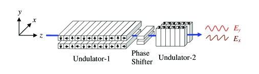
Figure 1: (color) Schematic of the crossed undulator for polarization control

In this section, we determine both SASE field components generated by the crossed undulator. Let $E(z,t)$ be the complex but slowly varying electric field at undulator distance $z$ and time $t$. We write

$$E(z,t)=\int{\omega_{1}d\nu\over\sqrt{2\pi}}E_{\nu}(z)e^{i\Delta\nu\left[(k_{1}+k_{u})z-\omega_{1}t\right]}\,,$$ (1)

where $\omega_{1}=k_{1}c$ is the fundamental resonant frequency corresponding to the average beam energy ($c$ is the speed of light); $\nu=\omega/\omega_{1}$ and $\Delta\nu=\nu-1$ is the relative frequency detuning, $k_{u}=2\pi/\lambda_{u}$ with $\lambda_{u}$ the undulator period. Following Refs. Kim_nim86 ; wang , the 1D FEL interaction starting from shot noise can be described by the coupled Maxwell-Klimontovich equations. In the small signal regime before FEL saturation, the equations can be linearized and solved by the Laplace transformation:

$$E_{\nu}(z) =\oint\frac{d\mu}{2\pi i}(-i2\rho k_{u})e^{-i2\rho\mu k_{u}z}E_{\nu,\mu}\,,$$

$$F_{\nu}(z) =\oint\frac{d\mu}{2\pi i}e^{-i2\rho\mu k_{u}z}\frac{\kappa_{1}E_{\nu,\mu}dV/d\eta-F_{\nu}(0)}{(\eta/\rho-\mu)}\,,$$ (2)

where

$$E_{\nu,\mu} =\frac{i}{2\rho k_{u}D(\mu)}\left(E_{\nu}(0)+\frac{i\kappa_{2}n_{0}}{2\rho k_{u}}\int d\eta\frac{F_{\nu}(0)}{\eta/\rho-\mu}\right)\,,$$

$$D(\mu) =\mu-\frac{\Delta\nu}{2\rho}-\int d\eta\frac{V(\eta)}{(\eta/\rho-\mu)^{2}}\,.$$ (3)

Here $E_{\nu}$ and $F_{\nu}$ are, respectively, the Fourier components of the electric field and of the Klimontovich distribution function that describes the discrete electrons in longitudinal phase space, with $E_{\nu}(0)$ and $F_{\nu}(0)$ the Fourier components of the initial conditions; $D(\mu)=0$ determines the FEL dispersion relation where $\mu$ is the Laplace parameter. In addition, parameter $\rho$ is the dimensionless FEL Pierce parameter BPN , $V(\eta)$ is the electron energy distribution with $\eta$ the relative energy deviation, $n_{0}$ is the electron volume density; $\kappa_{1}=eK\textrm{[JJ]}/(4\gamma_{0}^{2}mc^{2})$, $\kappa_{2}=eK\textrm{[JJ]}/(2\epsilon_{0}\gamma_{0})$, where $K$ is the dimensionless undulator strength parameter, the Bessel function factor [JJ] is equal to $[J_{0}(\xi)-J_{1}(\xi)]$ with $\xi=K^{2}/(4+2K^{2})$, $\gamma_{0}$ is the initial electron energy in units of $mc^{2}$, and $\epsilon_{0}$ is the vacuum permittivity. Note that the contour integration of $\mu$ in Eq. (II) must enclose all singularities in the complex $\mu$ plane. Based on this solution, we can calculate radiation field components in the crossed undulator according to their initial conditions.

II.1 Horizontal radiation field

The radiation field $E_{x}$ in the first undulator develops from electron shot noise, with the initial conditions

$$E_{\nu}^{x}(0)=0\,,\quad\int F_{\nu}^{x}(0)d\eta=\frac{1}{N_{\lambda}}\sum^{N_{e}}_{j=1}e^{i\nu\omega_{1}t_{j}(0)}\,,$$ (4)

where $N_{\lambda}$ is the number of electrons in one radiation wavelength, and $t_{j}(0)$ is the random arrival time of the $j^{th}$ electron at the entrance to the first undulator. We assume the first undulator operates in the exponential growth regime. In this regime, the dispersion relation has a solution $\mu_{0}$ with a positive imaginary part that gives rise to an exponentially growing field amplitude. For a cold beam with vanishing energy spread, we take $V(\eta)=\delta(\eta)$ in Eq. (II) and obtain

$$E_{\nu}^{x}(z) =\frac{-i\kappa_{2}n_{0}}{2\rho k_{u}N_{\lambda}3\mu_{0}}e^{-i\mu_{0}2\rho k_{u}z}\sum^{N_{e}}_{j=1}e^{i\nu\omega_{1}t_{j}}\quad\text{for $z\leq L_{1}$.}$$ (5)

In this high-gain regime, the electron distribution from Eq. (II) can be simplified as kim_nim445 :

$$F_{\nu}^{x}(z)=\frac{i\kappa_{1}E_{\nu}^{x}(z)dV/d\eta}{2k_{u}(-\mu_{0}\rho+\eta)}\quad\text{for $z\leq L_{1}$.}$$ (6)

This electron distribution function will be used as an initial condition for the calculation of the vertical radiation field as follows.

II.2 Vertical radiation field

The radiation field $E_{y}$ in the second undulator is generated by the pre-bunched electron beam in the first undulator. To control the radiation polarization, the required path length delay of the phase shifter chicane is on the order of the FEL wavelength. Such a weak chicane does not have dispersive effects that could result in micro-bunching, such as can be found for example in an optical klystron (see, e.g., Ref. OK ). Hence, the initial conditions at the entrance of the second undulator is

$$E_{\nu}^{y}(0)=0\,,\quad F_{\nu}^{y}(0)=F_{\nu}^{x}(L_{1})\,.$$ (7)

As the electron beam develops micro-bunching during the FEL interaction in the first undulator, it will radiate coherently in the second undulator. From discussions in Ref. kim_nim445 and simulation results shown in Sec. IV below, the intensity of $E_{y}$ can increase to the same level as that of $E_{x}$ in about one gain length. Thus, for a relatively short second undulator, we consider only coherent radiation and ignore any feedback of the radiation on the electron beam. With this approximation, the third term at the right hand side of $D(\mu)$ in Eq. (II) can be dropped, and Eq. (II) can now be written as

$$E_{\nu}^{y}(z_{2})= e^{i\phi}\oint\frac{d\mu}{2\pi i}\frac{e^{-i2\rho\mu k_{u}z_{2}}}{\mu-\Delta\nu/2\rho}\left[\frac{i\kappa_{2}n_{0}}{2\rho k_{u}}\int d\eta\frac{F_{\nu}^{x}(L_{1})}{\eta/\rho-\mu}\right]$$

$$= -e^{i\phi}\oint\frac{d\mu}{2\pi i}\frac{e^{-i2\rho\mu k_{u}z_{2}}}{\mu-\Delta\nu/2\rho}\frac{E_{\nu}^{x}(L_{1})}{\mu_{0}^{2}}\frac{\mu+\mu_{0}}{\mu^{2}}\,.$$ (8)

Here $z_{2}$ is the undulator distance from the beginning of the second undulator. The extra phase factor $e^{i\phi}$ is introduced by the phase shifter just before the second undulator. In the last step of Eq. (II.2), we have taken a cold beam with vanishing energy spread and made use of the relation $\kappa_{1}\kappa_{2}n_{0}=4k_{u}^{2}\rho^{3}$. Note that $\mu_{0}$ is the exponential growth solution that satisfies $D(\mu_{0})=0$ and is a function of the detuning parameter $\Delta\nu$, i.e.,

$$\mu_{0}\approx-{1\over 2}\left[1-{\Delta\nu\over 3\rho}+{(\Delta\nu)^{2}\over 36\rho^{2}}\right]+i{\sqrt{3}\over 2}\left[1-{(\Delta\nu)^{2}\over 36\rho^{2}}\right]\,.$$ (9)

Eq. (II.2) can be solved by the residue theorem:

$$E_{\nu}^{y}(z_{2})=E_{\nu}^{x}(L_{1})e^{i(\phi-\psi/2)}\textrm{sinc}\left({\psi\over 2}\right)\frac{2i}{\mu_{0}^{2}}\left[\rho k_{u}z_{2}-\mu_{0}e^{i\alpha}(\rho k_{u}z_{2})^{2}\right]\,,$$ (10)

where $\textrm{sinc}(x)=\sin(x)/x$, $\psi=\Delta\nu k_{u}z_{2}$, and

$$\alpha=\arctan\left[\frac{\textrm{sin}(\psi/2)}{\textrm{sinc}(\psi/2)-\textrm{cos}(\psi/2)}\right]\,.$$ (11)

Note that $\alpha=\pi/2$ when $\Delta\nu=0$. The first term in the square bracket of Eq. (10) describes coherent spontaneous radiation from a density-modulated beam and grows linearly with the undulator distance $z_{2}$ (as discussed in Ref. Yu in the context of harmonic generation). Since the electron beam from the first undulator possesses not only density modulation but also energy modulation, the momentum compaction of the second undulator can convert the energy modulation into additional density modulation. Thus, the second term in the square bracket of Eq. (10) describes the enhanced radiation due to the evolution of the density modulations inside the second undulator which grows quadratically with the undulator distance.

In order to generate circularly polarized light, we require that both $E_{x}$ and $E_{y}$ have the same average amplitude. From Eq. (10), this corresponds to the condition

$$\left|\frac{2i}{\mu_{0}^{2}}\left[\rho k_{u}z_{2}-\mu_{0}e^{i\alpha}(\rho k_{u}z_{2})^{2}\right]\right|=1\,.$$ (12)

We consider a cold electron beam with vanishing energy spread, hence the growth rate Im($\mu_{0}$) is maximized on resonance, i.e., $\Delta\nu=0$. In this case we obtain the required length of the second undulator from Eq.(12)

$$L_{2}\approx 1.3L_{G}\,,\quad\text{where}\quad L_{G}=\frac{\lambda_{u}}{4\pi\sqrt{3}\rho}$$ (13)

is the 1D power gain length.

III Degree of Polarization

The interference of the two radiation components generated by the crossed undulator will produce flexible polarization. At the end of the second undulator when $z=L_{1}+L_{2}$, these radiation fields in the time domain are

$$E_{y}(t)= \int{\omega_{1}d\nu\over\sqrt{2\pi}}E_{\nu}^{y}(z_{2}=L_{2})e^{i\Delta\nu\left[(k_{1}+k_{u})(L_{1}+L_{2})-\omega_{1}t\right]}\,,$$

$$E_{x}(t)= \int{\omega_{1}d\nu\over\sqrt{2\pi}}E_{\nu}^{x}(z=L_{1})e^{i\Delta\nu\left[(k_{1}+k_{u})L_{1}+k_{1}L_{2}-\omega_{1}t\right]}\,.$$ (14)

Note that we only used Eq. (1) for $E_{x}$ at $z=L_{1}$ (and $t_{1}$) and applied the free space propagation phase factor $e^{i\Delta\nu\left[k_{1}L_{2}-\omega_{1}(t-t_{1})\right]}$ in the second undulator as $E_{x}$ does not interact with the electron beam there. Because of the chaotic nature of SASE radiation, we perform a statistical analysis to quantify the state of polarization.

Following the standard optics textbooks (see, e.g., Refs. Born ; Goodman ), the state of polarization can be described by the coherency matrix

$${\mathbf{J}}=\left[\begin{array}[]{cc}\langle E_{x}(t)E_{x}^{*}(t)\rangle&\langle E_{x}(t)E_{y}^{*}(t)\rangle\\ \langle E_{y}(t)E_{x}^{*}(t)\rangle&\langle E_{y}(t)E_{y}^{*}(t)\rangle\\ \end{array}\right]\,,$$ (15)

where * means complex conjugate, and the angular bracket refers to the ensemble average. The degree of polarization can be calculated as Born ; Goodman

$$P\equiv\sqrt{1-4\frac{\textrm{det}[{\mathbf{J}}]}{(\textrm{tr}[{\mathbf{J}}])^{2}}}\,,$$ (16)

where $\textrm{det}[{\mathbf{J}}]$ and $\textrm{tr}[{\mathbf{J}}]$ are the determinant and trace of the coherency matrix, respectively. It is also convenient to introduce the first-order time correlation between $E_{x}$ and $E_{y}$ as

$$g_{xy}\equiv{\langle E_{x}(t)E_{y}^{*}(t)\rangle\over[\langle|E_{x}(t)|^{2}\rangle\langle|E_{y}(t)|^{2}\rangle]^{1/2}}.$$ (17)

For polarization control in the crossed undulator, we are particularly interested in the case when the average intensities of the two radiation components are the same: $\langle|E_{x}(t)|^{2}\rangle=\langle|E_{y}(t)|^{2}\rangle=\bar{I}$. Under this condition, the coherency matrix simplifies to

$${\mathbf{J}}=\bar{I}\left[\begin{array}[]{cc}1&|g_{xy}|e^{i\theta}\\ |g_{xy}|e^{-i\theta}&1\\ \end{array}\right]\,,$$ (18)

where $\theta$ is the phase difference between $E_{x}$ and $E_{y}$. When $\theta=\pm\frac{\pi}{2}$, the combined radiation is circularly polarized; when $\theta=0$ or $\pi$, it is linearly polarized at $\pm 45^{\circ}$ relative to the horizontal axis. The state of polarization is controllable by adjusting the phase shift $\phi$ in Eq. (10) so that the net phase in $g_{xy}$ is $\theta=\pm\frac{\pi}{2}$ or $0/\pi$. With equal intensity in both transverse directions, the degree of polarization in Eq. (16) is simply given by the amplitude of the $x$-$y$ time correlation, i.e.,

$$P=|g_{xy}|\,.$$ (19)

In the x-ray wavelength region, the electron bunch duration is typically much longer than the coherence time of the SASE radiation. Thus, a SASE pulse consists of many random intensity spikes that are statistically independent. For a flattop current distribution (of width $T$), we can convert the ensemble average of Eq. (17) into a time average as

$$g_{xy}= \lim_{T\rightarrow\infty}{1\over\bar{I}T}\int_{-T/2}^{T/2}dtE_{x}(t)E_{y}^{*}(t)$$

$$= {1\over\bar{I}T}\int_{-\infty}^{\infty}\omega_{1}d\nu E_{\nu}^{x}(L_{1})E_{\nu}^{y*}(L_{2})e^{-i\Delta\nu k_{u}L_{2}}\,,$$ (20)

where we have applied Eq. (III) and the Parseval relation in converting the time integration to the frequency integration. Assuming that the first undulator operates in the exponential gain regime, the frequency dependence of $E_{\nu}^{x}$ is approximately Gaussian, i.e.,

$$\langle|E_{\nu}^{x}(z)|^{2}\rangle=\frac{\bar{I}T}{\sqrt{2\pi}\sigma_{\omega}}e^{-\frac{(\Delta\nu)^{2}}{2\sigma_{\nu}^{2}}}\,,$$ (21)

where the relative rms SASE bandwidth is Kim_nim86 ; wang

$$\sigma_{\nu}=\sigma_{\omega}/\omega_{1}=\sqrt{9\rho\over\sqrt{3}k_{u}L_{1}}\,.$$ (22)

Since the short second undulator generates coherent radiation from a pre-bunched beam that possesses the same narrow bandwidth $\sigma_{\nu}$, we can expand $\mu_{0}^{2}$ in Eq. (10) to first order in $\Delta\nu$ by using Eq. (9). We also ignore the frequency dependence of the second term in the square bracket of Eq. (10) because its contribution to the radiation intensity is relatively small. Finally, we have

$$|g_{xy}|\approx\frac{1}{\sqrt{2\pi}}\Bigg{|}\int_{-\infty}^{\infty}d\bar{\nu}\frac{\exp\left(-{\bar{\nu}^{2}\over 2}-i{\bar{\nu}\sigma_{\nu}k_{u}L_{2}\over 2}\right)\textrm{sinc}\left({\bar{\nu}\sigma_{\nu}k_{u}L_{2}\over 2}\right)}{1+(-\frac{1}{2}+i\frac{\sqrt{3}}{2}){\bar{\nu}\sigma_{\nu}\over 3\rho}}\Bigg{|}\,,$$ (23)

where $\bar{\nu}=\Delta\nu/\sigma_{\nu}$. In view of Eq. (13), we take $L_{2}=1.3L_{G}$ in Eq. (23) and obtain the degree of polarization by computing $|g_{xy}|$.

IV Numerical simulations

IV.1 1D results

We first use a 1D FEL code to simulate the SASE radiation produced by the crossed undulator configuration and to analyze the degree of polarization. The code follows the time-dependent approach developed in Ref. bonifacio2 and employs the shot noise algorithm of Penman and McNeil penman . Electron energy spread can be included using Fawley’s beamlet method fawley . After computing the $E_{x}$ field produced in the first undulator, we allow $E_{x}$ to propagate freely without further interacting with the electron beam. The simulated electron distribution from the first undulator is then used to generate the $E_{y}$ field in the second undulator.

Table 1: Main parameters for the LCLS soft x-ray FEL used in simulations.

Parameter	value	unit
electron beam energy	4.3	GeV
relative energy spread	0(0.023)	%
bunch peak current	2	kA
transverse norm. emittance	1.2	$\mu$m
average beta function	8	m
undulator period $\lambda_{u}$	3	cm
undulator parameter $K$	3.5
FEL wavelength	1.509	nm
FEL $\rho$ parameter	0.119	%
1D power gain length $L_{G}$	1.17	m
3D power gain length $L_{G}^{3D}$	1.48	m

As a numerical example, we use the parameter set listed in Table 1 that is similar to the soft x-ray LCLS operation LCLS . In the 1D simulations, the energy spread is set to zero since we want to compare with the previous analytical results.

Fig. 2 shows the average radiation power in both $x$ and $y$ directions produced by the cross undulator. The length of the first undulator is allowed to vary, while the second undulator length $L_{2}=1.3L_{G}\approx 1.53$ m is held constant. As predicted by Eq. (13), the power of the two radiation components are essentially the same in the exponential gain regime. Near saturation, the power of the vertical field is lower than that of the horizontal one because the FEL-induced energy spread starts to de-bunch the electron beam in the second undulator. We repeat the simulations 200 times for each $L_{1}$ with different random seeds to start the process and calculate the first-order time correlation between $E_{x}$ and $E_{y}$ at the exit of the second undulator using the ensemble average defined in Eq. (17). Figure 3 shows the amplitude of this correlation from the simulation results as well as the numerical integration of Eq. (23) (the red solid curve) for a comparison. When the first undulator is less than a couple of gain lengths, the crossed undulator operates in the spontaneous emission regime, the amplitude of the $x$-$y$ correlation and hence the degree of polarization are very small without the use of a monochromator. The degree of polarization increases in the exponential growth regime and reaches a maximum of 85% near the FEL saturation. In this regime and especially when the gain is very high, we see very good agreement between simulations and Eq. (23). In the saturation regime, the amplitude of the $x$-$y$ correlation starts to decrease, and the linear theory starts to deviate from the simulation results.

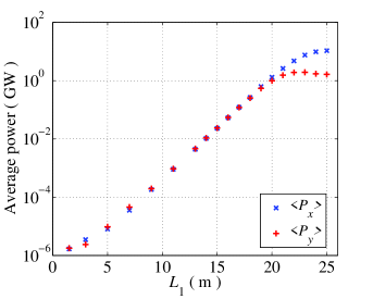
Figure 2: (color) 1D simulations of the average SASE power at 1.5 nm from the first (blue cross) and the second (red plus) undulator. Here $L_{1}$ is the length of the first undulator, $L_{2}=1.3L_{G}=1.53$ m is the length of the second undulator.

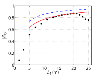
Figure 3: (color) Amplitude of the time correlation $|g_{xy}|$ from the 1D simulations (black star) and from Eq. (23) (red solid curve). The degree of polarization is equal to $|g_{xy}|$ when $\langle P_{x}\rangle=\langle P_{x}\rangle$. For comparison, the blue dashed curve shows an estimate of the polarization by Eq. (24) (see text for more details).

There are two effects that prevent the degree of polarization to reach 100% in a crossed-undulator SASE FEL. First, there is relative slippage between $E_{x}$ and $E_{y}$ in the second undulator. Since $E_{x}$ stops interacting with the electron beam after the first undulator, the group velocity of $E_{x}$ is the speed of light $c$. However, the group velocity of $E_{y}$ is slower than $c$ because it is generated by the micro-bunched beam that travels at the average longitudinal velocity $\beta_{\parallel}c$. In fact, 1D simulations indicate that the group velocity of $E_{y}$ is almost the same as that of the electrons within the short second undulator section. (This numerical result is also confirmed in 3D simulations to be discussed in the next section.) To estimate the slippage effect, we take $E_{y}(t)\approx E_{x}(t-\tau)$ with $c\tau=L_{2}(1-\beta_{\parallel})$ and apply the first-order time correlation function of the SASE field to estimate $|g_{xy}|$:

$$g(\tau)=\textrm{exp}\left(-{\pi\tau^{2}\over 2{\tau_{c}}^{2}}\right)\,,$$ (24)

where $\tau_{c}=\sqrt{\pi}/{\sigma_{\omega}}$ is the coherence time saldin , and $\sigma_{\omega}$ is given by Eq. (22). Equation (24) yields the blue dashed curve shown in Fig. 3, which indicates that the slippage effect only accounts for about a half of the depolarization in the crossed undulator. A careful examination of the intensity profile between $E_{x}$ and $E_{y}$ shows a visible difference from a simple time delay (see Fig. 4 for a 3D example). This accounts for the additional depolarization effect in a crossed undulator SASE FEL.

IV.2 3D Discussions

A remarkable feature of a SASE FEL is its transverse coherence. At a sufficiently high gain, a single transverse mode with the largest growth rate will dominate over all other transverse modes for a typical SASE FEL. Thus, we expect the previous 1D analysis still applies to 3D situations in the high gain limit, with the maximum polarization obtainable at the end of the exponential growth regime. Since the length of the second undulator is short, the diffraction effects for the free-propagating $E_{x}$ in the x-ray wavelength regime is expected to be small. Thus, the 3D effects such as emittance and diffraction do not play significant roles in determining the degree of polarization for a crossed undulator SASE FEL.

We use the 3D FEL code GENESIS 1.3 genesis to check these expectations. The electron beam is dumped at the end of the first undulator and is used to generate $E_{y}$ in the second undulator. $E_{x}$ propagates in the same length of the second undulator but without any undulator magnetic field. We use the same soft x-ray FEL example listed in Table 1 as the 1D case but with a relative energy spread of 0.023%, which roughly corresponds to the LCLS soft x-ray parameters. The length of the first undulator is chosen to be 23 m and is about 3 m before the saturation point. A 2-m short second undulator is necessary to produce the same radiation power for the vertical field (see Fig. 4). The 3D power gain length corresponding to these parameters is $L_{G}^{3D}=1.48$ m, so Eq. (13) approximately holds in this 3D case. We use the on-axis far-field radiation intensity and phase from GENESIS simulations to calculate the time correlation between $E_{x}$ and $E_{y}$ of Eq. (17). Instead of performing many statistical runs for the ensemble average, we average the result over hundreds of intensity spikes within the radiation pulse in order to save on simulation effort. The amplitude of the $x$-$y$ correlation from this 3D calculation is 87%, very close to the 1D prediction. Figure 4 shows the central section of the simulated power profiles $P_{x}$ and $P_{y}$ at the end of the second undulator. A small time delay due to the slippage effect and a somewhat different temporal structures between $P_{x}$ and $P_{y}$ are the main depolarization effects, as discussed in the previous section.

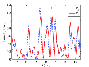
Figure 4: (color) GENESIS simulated power profiles of the horizontal field (blue dashed curve) and the vertical field (red solid curve) at the end of the second undulator, bunch head at left.

V Conclusions

The statistical analysis presented in this paper shows that the crossed-planar undulator is an effective method for polarization control in a SASE FEL. To optimize the degree of polarization, the first undulator should operate at the end of the exponential growth regime, while in order to generate circularly polarized x-rays, the second undulator should be about 1.3 times the power gain length. The maximum degree of polarization is over 80% from both theory and simulations. If fast pulsed magnets are employed in the phase shifter chicane, the relative phase between the two radiation components from the crossed undulator can vary at hundreds of Hz, hence enabling fast polarization switching for many scientific applications.

VI acknowledgments

We thank P. Emma, J. Hastings, and K.-J. Kim for many useful discussions. Special thanks to K. Bane for a careful reading of the manuscript and for his comments. This work was supported by Department of Energy Contract No. DE-AC02-76SF00515.

References

- (1) Linac Coherent Light Source Conceptual Design Report, SLAC-R-593, SLAC (2002).
- (2) TESLA Technical Design Report, TESLA FEL 2002-09, DESY (2002).
- (3) SPring-8 Compact SASE Source Conceptual Design Report, http://www-xfel.spring8.or.jp (2005).
- (4) S. Sasaki, Nucl. Instrum. Methods A 347, 83-86 (1994).
- (5) K.-J Kim, Nucl. Instrum. Methods A 219, 425 (1984).
- (6) K.-J. Kim, Nucl. Instrum. Methods A 445, 329 (2000).
- (7) J. Bahrdt, A. Gaupp, W. Gudat, M. Mast, K. Molter, W. B Peatman, M. Scheer, Th. Schroeter and Ch. Wang, Rev. Sci. Instrum. 63, 339 (1992).
- (8) J. Bahrdt, private communication.
- (9) Y.K. Wu, N.A. Vinokurov, S. Mikhailov, J. Li and V. Popov, Phys. Rev. Lett. 96, 224801 (2006).
- (10) K.-J Kim, Nucl. Instrum. Methods A 250, 396 (1986).
- (11) J. -M. Wang and L. -H. Yu, ibid, 484 (1986).
- (12) R. Bonifacio, C. Pellegrini and L.M. Narducci, Opt. Commun. 50, 373 (1984).
- (13) Y. Ding, P. Emma, Z. Huang and V. Kumar, Phys. Rev. ST Accel. Beams 9, 070702 (2006).
- (14) L.H. Yu, Phys. Rev. A 44, 5178 (1991).
- (15) M. Born and E. Wolf, Principles of Optics (Cambridge Universtiy Press, 7th ed., 1999).
- (16) J. Goodman, Statistical Optics (Wiley, 2000).
- (17) R. Bonifacio, B.W.J. McNeil, and P. Pierini, Phys. Rev. A 40, 4467 (1989).
- (18) C. Penman and B.W.J. McNeil, Opt. Commun. 90, 82 (1992).
- (19) W.M. Fawley, Phys. Rev. ST Accel. Beams 5, 070701 (2002).
- (20) E.L. Saldin, E.A. Schneidmiller and M.V. Yurkov, Opt. Commun. 148, 383 (1998).
- (21) S. Reiche, Nucl. Instrum. Methods A 429, 243 (1999).