the magneto-rotational instability near threshold: spatio-temporal amplitude equation and saturation

Abstract

We show, by means of a perturbative weakly nonlinear analysis, that the axisymmetric magneto-rotational instability (MRI) in a magnetic Taylor-Couette (mTC) flow in a thin-gap gives rise, for very small magnetic Prandtl numbers (${\cal P}_{\rm m}$), to a real Ginzburg-Landau equation for the disturbance amplitude. The saturation amplitude $A_{s}$ is found to scale in this regime as ${\cal P}_{\rm m}^{\delta}$, with $1/2<\delta<2/3$ (depending on the boundary conditions adopted). The asymptotic results are shown to comply with numerical calculations performed by using a spectral code. They suggest that the transport due to the nonlinearly developed MRI may be vanishingly small for ${\cal P}_{\rm m}\ll 1$.

1 Introduction

1.1 General

Asymptotic approaches to nonlinear stellar pulsation were pioneered by Robert Buchler and his collaborators (see this volume). Amplitude equations, which capture the essential dynamics near the instability threshold, result from such approaches and may usually be derived using singular perturbation theory (see Marie-Jo Goupil, this volume). In this contribution we report on the results of applying a perturbative asymptotic analysis to an instability that has acquired, in the past 15 years or so, a paramount importance in the quest to understand angular momentum transport in accretion disks, namely the magneto-rotational instability (MRI). Even though the system studied here is rather different from pulsating stars, the ideas and techniques are quite similar. One important difference is that while the amplitude equations for stellar pulsation are sets of ordinary differential equations, here we must take recourse to partial differential equation(s) (PDE), in which the amplitude (usually called in this case envelope) is a function of time (as in the ordinary amplitude equations) and space. The application of singular perturbation theory requires thus the use of slow variation in time as well as in space. In this way spatio-temporal slow dynamics (i.e., patterns) is captured by a generic PDE - the real Ginzburg-Landau Equation, rGLE, in our case.

The rudiments of singular perturbation theory are well explained in the book by Bender & Orszag ([1999]), while a detailed account on problems dealing with the dynamics on the center manifold can be found in Manneville ([1990]). It seems that these powerful analytical and semi-analytical techniques have not yet found their way to enough astrophysical applications. In the early 1980s Robert Buchler started an ambitious program of introducing such a new approach to stellar pulsation. I was fortunate to be his postdoc then, but have moved on to other topics. Robert and his postdocs (most of which contributed to this volume) have pursued this program and during this conference one could learn just how much has been achieved in the understanding of stellar pulsation, following asymptotic approaches, combined with numerical and phenomenological ones. It is quite unfortunate that ”driving forces” of Robert’s magnitude have unfortunately been quite rare in other branches of astrophysics.

1.2 The MRI - background

The linear MRI has been known for almost 50 years (Velikhov [1959], Chandrasekhar [1960]): Rayleigh stable rotating Couette flows of conducting fluids are destabilized in the presence of a vertical magnetic field if $d\Omega^{2}/dr<0$ (angular velocity decreasing outward). However, the MRI only acquired importance to astrophysics after the influential work of Balbus & Hawley ([1991]), who demonstrated its viability to cylindrical accretion disks (for any sufficiently weak field). The linear analysis was later supplemented by nonlinear numerical simulations (albeit of a small, shearing-box (SB), segment of the disk). Enhanced transport (conceivably turbulent) is necessary for accretion to proceed in disks, found in a variety of astrophysical settings - from protostars to active galactic nuclei. As is well known, Keplerian rotation law is hydrodynamically linearly stable and thus the MRI has been widely accepted as an attractive solution for enhanced transport (see the reviews by Balbus & Hawley [1998] and Balbus [2003]), even though some questions on the nature of MRI-driven turbulence still remain (see, e.g., Branderburg [2005]), in particular in view of some recent numerical studies (Pessah, Chan & Psaltis [2007], Fromang & Papaloizou [2007], Fromang et al. [2007]). Because of the MRI’s importance and some of its outstanding unresolved issues, several groups have quite recently undertaken projects to investigate the instability under laboratory conditions. Additionally, numerical simulations specially designed for experimental setups have been conducted. It appears, however, quite impossible to make definite deductions from these experiments and simulations (see, e.g., Ji et al. [2001], Noguchi et al. [2002], Sisan et al. [2004], Stefani et al. [2006], and references therein).

We shall report here on the result of a weakly nonlinear analysis of the MRI near threshold, for a dissipative mTC flow. We have done the analysis for the above simplified (relatively to an accretion disk) problem for two types of boundary conditions (see Umurhan, Menou & Regev [2007], hereafter UMR and Umurhan, Regev & Menou [2007], hereafter URM, for a detailed account). This kind of approach is important because the viability of the MRI as the driver of turbulence and angular-momentum transport relies on understanding its nonlinear development and saturation. By complementing numerical simulations with analytical methods useful physical insight can be expected. To facilitate an analytical approach we made a number of simplifying assumptions so as to make the system amenable to well-known asymptotic methods (see, e.g., Cross and Hohenberg [2003], Regev [2006]) for the derivation of a nonlinear envelope equation, valid near the linear instability threshold.

2 Linear theory

2.1 Equations

The hydromagnetic equations in cylindrical coordinates (Chandrasekhar [1961]) are applied to the neighborhood of a representative radial point ($r_{0}$) in a mTC setup with an imposed constant background vertical magnetic field. The steady base flow has only a constant vertical magnetic field, ${\bf B}=B_{0}{\bf\hat{z}}$, and a velocity of the form ${\bf V}=U(x){\bf{\hat{y}}}$. In this base state the velocity has a linear shear profile $U(x)=-q\Omega_{0}x$, representing an azimuthal flow about a point $r_{0}$, that rotates with a rate $\Omega_{0}$, defined from the differential rotation law $\Omega(r)\propto\Omega_{0}(r/r_{0})^{-q}$ ($q=3/2$ for Keplerian rotation). The total pressure in the base state (divided by the constant density), $\Pi\equiv{\rho_{0}}^{-1}\left(P+\frac{B_{0}^{2}}{8\pi}\right)$, is a constant and thus its gradient is zero.

This base flow is disturbed by 3-D perturbations on the magnetic field ${\bf b}=(b_{x},b_{y},b_{z})$, as well as on the velocity - ${\bf u}=(u_{x},u_{y},u_{z})$, and on the total pressure - $\varpi$. We consider only axisymmetric disturbances, i.e. perturbations with structure only in the $x$ and $z$ directions. This results, after non-dimensionalization, in the following set of equations, given here in the rotating frame:

$$\frac{d{\bf u}}{dt}-2{{\Omega_{0}\bf{\hat{z}}}\times{\bf u}}-{q\Omega_{0}u_{x}{\bf{\hat{y}}}}-{\cal C}{\bf b}\cdot\nabla{\bf b}-{\cal C}B_{0}\partial_{z}{\bf b} = -\nabla\varpi+\frac{1}{{\cal R}}\nabla^{2}{\bf u},$$ (1)

$$\frac{d{\bf b}}{dt}-{\bf b}\cdot\nabla{\bf u}+{q\Omega_{0}b_{x}{\bf{\hat{y}}}}-B_{0}\partial_{z}{\bf u} = \frac{1}{{\cal R}_{{m}}}\nabla^{2}{\bf b},$$ (2)

$$\nabla\cdot{\bf u}\equiv\partial_{x}u_{x}+\partial_{z}u_{z}=0,\qquad\nabla\cdot{\bf b}\equiv\partial_{x}b_{x}+\partial_{z}b_{z}=0.$$ (3)

The Cartesian coordinates $x,y,z$ correspond to the radial (shear-wise), azimuthal (stream-wise) and vertical directions, respectively, and since axisymmetry is assumed $\nabla\equiv{\bf\hat{x}}\partial_{x}+{\bf\hat{z}}\partial_{z}$ and $\nabla^{2}\equiv\partial_{x}^{2}+\partial_{z}^{2}$. Lengths have been non-dimensionalized by $L$ ($\approx$ the gap size), time by the local rotation rate $\tilde{\Omega}_{0}$ (tildes denote dimensional quantities). Because the dimensional rotation rate of the box (about the central object) is ${\bf\tilde{\Omega}_{0}}=\tilde{\Omega}_{0}{\bf\hat{z}}$, the non-dimensional quantity $\Omega_{0}$ is simply equal to $1$, but we keep it to flag the Coriolis terms. Velocities have been scaled by $\tilde{\Omega}_{0}L$ and the magnetic field by its background value $\tilde{B}_{0}$. Thus $B_{0}\equiv 1$ as well, but again, we leave it in the equation set for later convenience. The hydrodynamic pressure is scaled by $\tilde{\rho}_{0}L^{2}\tilde{\Omega}_{0}^{2}$ and the magnetic one by $\tilde{B}_{0}^{2}/(8\pi)$. The non-dimensional perturbation $\varpi$ of the total pressure divided by the density (which is equal to 1 in non-dimensional units), which survives the spatial derivatives, is thus given by $\varpi=p+{\cal C}\mbox{$\frac{1}{2}$}|{\bf b}|^{2}$, where $p$ is the hydrodynamic pressure perturbation. The non-dimensional parameter ${\cal C}\equiv\tilde{B}_{0}^{2}/(4\pi\tilde{\rho}_{0}\tilde{\Omega}_{0}^{2}L^{2})=\tilde{V}_{A}^{2}/\tilde{V}^{2}$ is the Cowling number, measuring the relative importance of the magnetic pressure to the hydrodynamical one. It is equal to the inverse square of the typical Alfvén number ($\tilde{V}_{A}$ is the typical Alfvén speed). The Cowling number appears in the non-linear equations, together with the two Reynolds numbers: ${\cal R}\equiv{\tilde{\Omega}_{0}L^{2}}/{\tilde{\nu}}$ and ${\cal R}_{m}\equiv{\tilde{\Omega}_{0}L^{2}}/{\tilde{\eta}}$, where $\tilde{\nu}$ and $\tilde{\eta}$ are, respectively, the microscopic viscosity and magnetic resistivity of the fluid. We shall also see that the magnetic Prandtl number, given as ${\cal P}_{m}\equiv{\cal R}_{m}/{\cal R}$, plays an important role in the nonlinear evolution of this system.

It is useful to rewrite the above equations of motion in terms of more convenient dependent variables. Because the flow is incompressible and $y$-independent, the radial and vertical velocities can be expressed in terms of the streamfunction, $\Psi$, that is, $(u{{}_{x}},u{{}_{z}})=(\partial_{z}\Psi,-\partial_{x}\Psi)$. Also, since the magnetic field is source free, one can similarly express its vertical and radial components in terms of the flux function, $\Phi$, that is, $(b{{}_{x}},b{{}_{z}})=(\partial_{z}\Phi,-\partial_{x}\Phi)$ (see URM for details). The system is supplement by appropriate boundary condition on the thin cylindrical gap ”walls”, as detailed in UMR and URM and we also point out that the stress relevant for angular momentum transport, $\Sigma$, is

$${\Sigma}={\Sigma}_{\rm R}+{\Sigma}_{\rm M},\qquad{\Sigma}_{\rm R}\equiv u_{x}u_{y},\quad{\Sigma}_{\rm M}\equiv-{\cal C}b_{x}b_{y}.$$

which consists of ${\Sigma}_{\rm R}$ and ${\Sigma}_{\rm M}$, the Reynolds (hydrodynamic) and Maxwell stresses, expressing the velocity and magnetic field disturbance correlations, respectively.

2.2 Linear stability

Linearization of (2.1-2.3), for perturbations of the form $\propto e^{st+ik_{x}x+ik_{z}z}$, gives rise to the dispersion relation,

$${\cal D}(s;k_{x},k_{z},{\cal P}_{\rm m},{\cal S},{\cal C},q)=a_{0}s^{4}+a_{1}s^{3}+a_{2}s^{2}+a_{3}s+a_{4}=0,$$

where all the $a_{i}$ are functions of $k_{x}$, $k_{z}$ and the other parameters, but we shall write explicitly only the coefficient that will be used in what follows,

$$a_{4}=\frac{{\cal C}}{{\cal S}^{4}}\Bigl{[}k_{{}_{T}}^{2}{\cal C}({\cal C}k_{{}_{T}}^{4}{\cal P}_{\rm m}+k_{z}^{2}{\cal S}^{2})^{2}+\kappa^{2}{\cal S}^{2}{\cal C}k_{{}_{T}}^{4}k_{z}^{2}-2q{\cal S}^{4}k_{z}^{4}\Bigr{]},$$ (4)

where the notation $\kappa^{2}\equiv 2(2-q),\ k_{{}_{T}}^{2}\equiv k_{x}^{2}+k_{z}^{2}$ is introduced.

For given values of the parameters (call them $p_{j}$) there will be four distinct modes. The linear theory in various limits for this problem has been discussed in numerous publications and we shall not elaborate upon it any further. Rather, we focus on situations where the most unstable mode (of the four) is marginal (critical) for some $k_{z}$ at a given value of $k_{x}=K$. We fix $K$ in order to focus on the marginal vertical dynamics within the thin gap (actually a rotating channel, see below). Marginality ($s=0$) implies the vanishing of the real coefficient $a_{4}(k_{z})$ (as expressed above) and its derivative with respect to $k_{z}$ at some $k_{z}=Q$:

$$a_{4}(k_{z}=Q;K,p_{j})=0,\qquad\frac{\partial a_{4}}{\partial k_{z}}(k_{z}=Q;K,p_{j})=0.$$ (5)

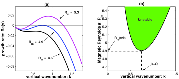
Figure 1: Summary of linear theory. This example is for ${\cal C}=0.08$, ${\cal P}_{m}=0.001$, $q=3/2$, and the fundamental mode. (a) Growth rates, $Re(s)$, as a function of wavenumber $k$ for three values of ${\cal R}_{m}$. (b) Solid line depicts those values of ${\cal R}_{m}$ and $k$ where $Re(s)=0$. The shaded region shows unstable modes. The locations of $k=k_{crit}\equiv Q$ and ${\cal R}_{m}={\cal R}_{m}({\rm crit})\equiv R_{m}$ are shown.

The second condition and (4) yield

$$Q\Bigl{[}Q^{2}{\cal S}^{4}({\cal C}Q^{2}-4q)+(K^{2}+Q^{2})2Q^{2}{\cal C}{\cal S}^{2}({\cal S}^{2}+\kappa^{2})+$$

$$(K^{2}+Q^{2})^{2}{\cal C}{\cal S}^{2}(6{\cal C}{\cal P_{\rm m}}Q^{2}+\kappa^{2})+$$

$$2(K^{2}+Q^{2})^{3}{\cal P_{\rm m}}{\cal C}^{2}{\cal S}^{2}+5(K^{2}+Q^{2})^{4}{\cal P_{\rm m}}^{2}{\cal C}^{3}\Bigl{]}=0.$$ (6)

This equation, together with $a_{4}(k_{z}=Q,K;p_{i})=0$, can be solved for ${\cal S}$ and $Q$. The general expressions for ${\cal S}(K,{\cal P}_{\rm m},{\cal C},q)$ and $Q(K,{\cal P}_{\rm m},{\cal C},q)$ are lengthy but their asymptotic forms, to ${\cal O}\left({{\cal P}_{\rm m}}\right)$ (for ${\cal P}_{\rm m}\ll 1$), are simple,

$${\cal S}=\frac{\sqrt{16\ {\cal C}q(2-q)}K}{(2q-{\cal C}K^{2})},\qquad Q^{2}=K^{2}\frac{2q-{\cal C}K^{2}}{2q+{\cal C}K^{2}}$$ (7)

If ${\cal C}K^{2}>2q$ the solutions are not physically meaningful, while ${\cal C}K^{2}=2q$ corresponds to the ideal MRI limit.

Our system is a rotating thin channel, whose walls are at $x=0,\pi/K$. All quantities are vertically periodic on a scale $L_{z}$ commensurate with integer multiples of $2\pi/Q$. As long as $L_{z}\gg 1/Q$, the limit of a vertically extended system (and thus a continuous spectrum of vertical modes) may be effected. Linear theory, as discussed above, is summarized in Figure 1

3 Weakly nonlinear analysis

We follow the fluid into instability by tuning the vertical background field away from the steady state, i.e. $B_{0}\rightarrow 1-\epsilon^{2}\tilde{\lambda},$ where $\epsilon\ll 1$ and $\tilde{\lambda}$ is an ${\cal O}\left({1}\right)$ control parameter. This means that we are now in a position to apply procedures of singular perturbation theory to this problem, by employing the multiple-scale (in $z$ and $t$) method (e.g, Bender & Orszag [1999]). It facilitates, by imposing suitable solvability conditions at each expansion order of the calculation in order to prevent a breakdown in the solutions, a derivation of an envelope equation for the unstable mode. Thus for any dependent fluid quantity $F(x,z,t)$ we assume

$$F(x,z,t)=\epsilon F_{1}(x,z,t)+\epsilon^{2}F_{2}(x,z,t)+\cdots.$$ (8)

The fact that the $x$ and $z$ components of the velocity and magnetic field perturbations can be derived from a streamfunction, $\Psi(x,z)$ and magnetic flux function $\Phi(x,z)$ reduces the number of relevant dependent variables $F$ to four ($u_{y}$ and $b_{y}$ are the additional two). These four dependent variables will also be used in the spectral numerical calculation (see below).

For the lowest $\epsilon$ order of the equations, resulting from substituting the expansions into the original PDE and collecting same order terms, we make the Ansatz $F_{1}(x,z,t)=\hat{F}_{1}\tilde{A}(\epsilon z,\epsilon^{2}t)e^{iQz}\sin Kx+{\rm c.c.},$ where $\hat{F}_{1}$ is a constant (according to the variable in question), and where the envelope function $\tilde{A}$ (an arbitrary constant amplitude in linear theory) is now allowed to have weak space (on scale $Z\equiv\epsilon z$) and time (on scale $T\equiv\epsilon^{2}t$) dependencies. Because this system is tenth order in $x$-derivatives, a sufficient number of conditions must be specified at the edges. and the Ansatz has to obey them. In UMR we chose mathematically expedient boundary conditions, which allowed fully analytical treatment for the limit ${\cal P}_{\rm m}\ll 1$ and here we shall report, in some detail, only on the results of that work. We have also tried some different boundary conditions (see URM) and in that case the rGLE coefficients had to be calculated numerically. The qualitative behavior of the saturation amplitude was found to be quite similar (see below).

3.1 Real Ginzubrg-Landau equation

The end result of the asymptotic procedure procedure is the well-known real Ginzburg-Landau Equation (rGLE) which, for ${\cal P}_{\rm m}\ll 1$, is

$$\partial_{T}A=\lambda A-\frac{1}{{\cal P}_{\rm m}{\cal C}}|A|A^{2}+D\partial_{{}_{Z}}^{2}A.$$ (9)

We shall consider only the magnitude (real part) of $A$. In a 1D gradient system like this one phase dynamics can only give rise to wavelength modulations and consequently our main results are in no way affected by it. The real envelope is $A\equiv{\sqrt{\xi}}\tilde{A}$, $\lambda\equiv\zeta\tilde{\lambda}$, and the coefficients, for $q=3/2$ are

$$\xi = \frac{3}{4}\cdot\frac{5{\cal S}^{4}-18{\cal S}^{2}-32+2({\cal S}^{2}+16)\sqrt{{\cal S}^{2}+1}}{{\cal S}({\cal S}^{2}+1)(4\sqrt{{\cal S}^{2}+1}-3)},\ \ \$$ (10)

$$D = 6\frac{\left({\cal S}^{2}+2-2\sqrt{{\cal S}^{2}+1}\right)({\cal S}^{2}+1)}{{\cal S}^{3}(4\sqrt{{\cal S}^{2}+1}-3)},$$ (11)

$$\zeta = \frac{3{\cal S}\sqrt{{\cal S}^{2}+1}-6{\cal S}}{4{\cal S}^{2}+1+\sqrt{{\cal S}^{2}+1}},$$ (12)

where ${\cal S}(K)$ is as given in (7). For ${\cal S}\gg 1$, (i.e. as one approaches the ideal MRI limit), these simplify to $\xi=15/16,\ \zeta=3/4,\ D=3/2$; and in general they remain ${\cal O}\left({1}\right)$ quantities for all reasonable values of ${\cal S}$.

3.2 Scaling of angular momentum transport

Contributions to the total angular momentum transport ($\dot{\rm J}=\dot{\rm J}_{\rm H}+\dot{\rm J}_{\rm B}$) due to the hydrodynamic ($\dot{\rm J}_{\rm H}$) and magnetic correlations ($\dot{\rm J}_{\rm B}$) are, to leading order,

$$\dot{\rm J}_{\rm H} = \frac{9\epsilon^{2}}{{\cal S}}\left(\frac{2+{\cal S}^{2}-2\sqrt{1+{\cal S}^{2}}}{1+{\cal S}^{2}}\right)A^{2}+{\cal O}\left({\epsilon^{3},\epsilon^{2}{\cal P}_{\rm m}}\right),\ \ \ \ \$$

$$\dot{\rm J}_{\rm B} = \frac{3\epsilon^{2}}{{\cal S}}\left(1-\frac{1}{\sqrt{1+{\cal S}^{2}}}\right)A^{2}+{\cal O}\left({\epsilon^{3},\epsilon^{2}{\cal P}_{\rm m}}\right).$$ (13)

The envelope $A$ is found by solving the rGLE, which is a well-studied system (see, e.g., Regev [2006], for a summary and references). It has 3 steady uniform solutions in 1D (here, the vertical): an unstable state $A=0$, and 2 stable states $A=\pm A_{s}$, where $A_{s}^{2}=|\zeta({\cal S})|{\cal P}_{\rm m}{\cal C}$ (note that $\zeta({\cal S})$ is an ${\cal O}\left({1}\right)$ quantity). $A_{s}$ is also the saturation amplitude, because the system will develop towards it.

Setting $A\rightarrow A_{s}$ in (13) and in the expression for ${\rm E_{V}}$ (the total disturbance energy, see UMR), followed by some algebra, reveals that the angular momentum flux in the saturated state is, to leading order in ${\cal P}_{\rm m}$ and $\epsilon$, $\dot{\rm J}=\epsilon^{2}|\zeta({\cal S})|\gamma({\cal S}){\cal P}_{\rm m}{\cal C}{\cal S}^{-1}$, while in the expression for the energy one term is independent of ${\cal P}_{\rm m}$, ${\rm E_{V}}=\epsilon^{4}{\cal C}^{3}\zeta^{2}({\cal S})\beta_{2}({\cal S})+{\cal O}\left({{\cal P}_{\rm m}}\right)$. The key results of this analysis (see URM) are the following scalings (with the magnetic Prandtl number)

$$A_{s}\sim\sqrt{\cal P}_{\rm m}\longrightarrow{\rm E_{V}}\sim E_{0},~{}~{}~{}~{}\dot{\rm J}\sim{\cal P}_{\rm m}$$ (14)

for ${\cal P}_{\rm m}\ll 1$, where $E_{0}$ is a constant, independent of ${\cal P}_{\rm m}$ . For fixed resistivity this implies $\dot{\rm J}\sim{\cal R}^{-1}$.

We have also performed fully numerical calculations, using a 2-D spectral code to solve the original nonlinear equations, in the streamfunction and magnetic flux function formulation, near MRI threshold. The code implemented a Fourier-Galerkin expansion in ${\rm 64}\times{\rm 64}$ modes in each of the four independent physical variables, i.e. ${\bf F}=\sum_{n,m}{\bf F}_{\rm nm}(t)\sin K_{n}xe^{iQ_{m}z}+{\rm c.c.}$, where ${\bf F}=(\psi,u_{y},\Phi,b_{y})^{{\rm T}}$ and where ${\bf F}_{\rm nm}(t)$ is the time-dependent amplitude of the particular Fourier-Galerkin mode in question (denoted by the indices $n,m$). We typically started with white noise initial conditions on ${\bf F}_{\rm nm}(0)$ at a level of 0.1 the energy of the background shear. Because of space limitations we display only a representative plot of runs made with ${\cal S}=5.0$, ${\cal C}=0.05$, (i.e. ${\cal R}_{\rm m}$ fixed), $q=3/2$ and $\epsilon^{2}=0.2$ for a few successively increasing values of ${\cal R}$ (Figure 2). With this value of $\epsilon$ the fastest growing linear mode has a growth rate of $\sim 0.065$, and thus fully developed ideal MRI can not be expected.

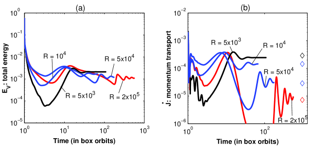
Figure 2: ${\rm E_{V}}$ (panel a) and $\dot{\rm J}$ (panel b) as a function of time from numerical calculation. The different lines are labeled by the value of the Reynolds number ${\cal R}$ The diamonds in panel (b) show the scaling predicted by our asymptotic analysis, predicting also a constant final value of the disturbance energy, as apparent in panel (a). One ”box orbit” $=2\pi$ in nondimensional units.

${\rm E}_{\rm V}$ saturates at a constant independent of ${\cal R}$ (for small enough ${\cal P}_{\rm m}$), while $\dot{\rm J}$ saturates at values that scale as ${\cal R}^{-1}$. Thus the asymptotic analysis fits very well the fully numerical results after the system saturates.

4 Summary

The numerical and asymptotic solutions developed here show that for ${\cal P}_{\rm m}\ll 1$, it is the azimuthal velocity perturbation, arising from the ${\cal O}\left({\epsilon^{2}}\right)$ term, that becomes dominant in the saturated state. It appears to be the primary agent in the nonlinear saturation of the MRI in the channel, acting anisotropically so as to modify the shear profile and results in a non-diagonal stress component (relevant for angular momentum transport). Our analysis is complementary to the study of Knobloch and Julien ([2005]), who have performed an asymptotic MRI analysis, but for a developed state, far from marginality.

The trends predicted by this simplified model are not qualitatively altered by different boundary conditions, the value of $\delta$ changing only by a small amount. Qualitatively similar scalings, but with somewhat different values of $\delta>0$, have very recently been reported by Lesur & Longaretti ([2007]) and Fromang et al. ([2007]), however in those SB simulations ${\cal P}_{\rm m}$ was not taken to be vanishingly small. It should be remarked that conventional accretion disks do have ${\cal P}_{\rm m}\ll 1$, but the numerical SB simulations cannot faithfully treat very small such Prandtl numbers, for numerical reasons. Further analytical investigations of the kind reported here should contribute to better physical understanding of the MRI saturation..

References

- [2003] Balbus, S.A. 2003, ARA&A, 41, 555
- [1991] Balbus, S.A. and Hawley, J.F. 1991, ApJ, 376, 214
- [1998] Balbus, S.A. and Hawley, J.F. 1998, Rev. Mod. Phys., 70, 1
- [1999] Bender, C.M. and Orszag, S.A. 1999, Advanced Mathematical Methods for Scientists and Engineers, Springer, New York
- [2005] Brandenburg, A. 2005, Astron. Nachr., 326, 787.
- [1960] Chandrasekhar, S. 1960, Proc. Natl. Acad. Sci. USA, 46, 253.
- [1961] Chandrasekhar, S. 1961, Hydrodynamic and Hydromagnetic Stability, Oxford University Press, Oxford
- [2003] Cross, M.C. and Hohenberg, P.C. 2003, Rev. Mod. Phys. 65, 851
- [2007] Fromang, S. and Papaloizou, J. 2007, A&A, 476, 1113
- [2007] Fromang, S., Papaloizou, J., Lesur, G. and Heinemann, T. 2007, A&A, 476, 1123
- [2001] Ji, H., Goodman, J. and Kageyama, A. 2001, MNRAS, 325, L1
- [2005] Knobloch, E. & Julien, K. 2005, Phys. Fluids, 17, 094106
- [2007] Lesur, G., & Longaretti, P.-Y. 2007, MNRAS, 378, 1471
- [1990] Manneville, P. 1990, Dissipative Structures and Weak Turbulence, Academic Press, Boston
- [2002] Noguchi, K., Pariev, V.A., Colgate, S.A., Beckley, H.F. and Nordhaus, J. 2002, ApJ, 575, 1151
- [2007] Pessah, M.E., Chan, C-k. & Psaltis, D. 2007, ApJ , 668, L51
- [2006] Regev, O. 2006, Chaos and Complexity in Astrophysics, Cambridge University Press, Cambridge
- [2004] Sisan, D.R., Mujica, N., Tillotson, W.A., Huang, Y., Dorland, W., Hassam, A.B., Antonsen, T.M. and Lathrop, D.P., 2004, Phys. Rev. Lett., 93, 114502
- [2006] Stefani, F., Gundrum, T., Gerbeth, G., R diger, G., Schultz, M., Szklarski, J. and Hollerbach, R., 2006, Phys. Rev. Lett., 97, 184502
- [2004] Umurhan, O.M. and Regev, O. 2004, A&A, 427, 855.
- [2007] Umurhan, O.M., Menou, K. & Regev, O. 2007, Phys. Rev. Lett., 98, 034501
- [2007] Umurhan, O.M., Regev, O. & Menou, K. 2007, Phys. Rev. E, 76, 036310
- [1959] Velikhov, E.P. 1959, Sov. Phys. JETP, 9, 959.