Response, relaxation and transport
in unconventional superconductors

Abstract

We investigate the collision–limited electronic Raman response and the attenuation of ultrasound in spin–singlet $d$–wave superconductors at low temperatures. The dominating elastic collisions are treated within a t–matrix approximation, which combines the description of weak (Born) and strong (unitary) impurity scattering. In the long wavelength limit a two–fluid description of both response and transport emerges. Collisions are here seen to exclusively dominate the relaxational dynamics of the (Bogoliubov) quasiparticle system and the analysis allows for a clear connection of response and transport phenomena. When applied to quasi–2–$d$ superconductors like the cuprates, it turns out that the transport parameter associated with the Raman scattering intensity for B_1g and B_2g photon polarization is closely related to the corresponding components of the shear viscosity tensor, which dominates the attenuation of ultrasound. At low temperatures we present analytic solutions of the transport equations, resulting in a non–power–law behavior of the transport parameters on temperature.

PACS: 67.57.Hi 74.20.-z 74.20.Fg 74.20.Rp 74.25.Fy 74.25.Ld

1 Introduction

During the last few decades a large variety of so–called unconventional superconductors have been discovered, among these the superfluid phases of ³He [1, 2, 3, 4], the heavy Fermion systems[5, 6, 7], the cuprates[8, 9] and the Ruddlesden–Popper system Sr₂RuO₄[10]. The unconventional pairing correlations in these systems manifest themselves on the one hand in an anisotropy of the pair potential or energy gap of less symmetry than the underlying band structure or in the occurrence of additional spontaneously broken symmetries besides the $U(1)$ gauge symmetry. On the other hand their existence can be detected from the sensitivity of thermodynamic quantities like the transition temperature or the equilibrium energy gap to even small amounts of non–magnetic impurities.

In an earlier publication [11], a simple two–fluid description for these unconventional superconductors was formulated, which emerges from the BCS theory in the long wavelength (${\bf q}\to 0$) and stationary ($\omega\to 0$) limit, sometimes also referred to as the local equilibrium. As a result, even analytical results were obtained for the temperature dependence of the local reactive response functions of the normal component, the Bogoliubov quasiparticles (specific heat capacity, spin susceptibility) and the condensate (superfluid density, magnetic penetration depth). Clearly, a comprehensive two–fluid description of superconductors should describe the more general situation beyond local equilibrium and should therefore contain the dissipative response of both the quasiparticle system and the condensate. A first step in this direction was the derivation of a general form of a certain class of quasiparticle transport parameters for unconventional superconductors in reference [12]. The results for the impurity–limited transport of momentum (shear viscosity) and energy (diffusive thermal conductivity) were, however, discussed exclusively for the case of superfluid ³He–B with silica aerogel forming the impurity system. Moreover, the two aspects of response and transport traditionally appear as fairly remote aspects of the reactive and dissipative dynamics of a superconductor.

Therefore, this paper is devoted to a unified description of response and transport in superconductors. To be specific, we limit our considerations to unconventional spin–singlet superconductors with $d$–wave pairing correlations, in view of an applicability to hole–doped cuprate superconductors. We would furthermore like to concentrate on the electronic Raman [13] and stress tensor response. When treated in the long wavelength limit, the corresponding response functions can be shown to be separable into normal (Bogoliubov quasiparticles) and superconducting (pair condensate) contributions, respectively, hence allowing for a two–fluid description at arbitrary quasiclassical frequencies in the homogeneous (${\bf q}\to 0$) limit. While the dynamics of the condensate can be characterized by some pseudo–conservation laws governing the macroscopic phase of the order parameter (reactive response), as well as by pair–breaking processes (dissipative response), the system of Bogoliubov quasiparticles shows purely relaxational behavior in the long wavelength limit. For a quantitative study of the latter behavior we consider impurity–limited transport, believed to dominate at low temperatures. Collisions of the BQP with impurities are treated within the t–matrix approximation [14, 17, 18, 19], which is limited here to s–wave scattering. The description thus allows one to treat the cases of weak scattering (Born limit, $\delta_{0}\to 0$) and strong scattering (unitary limit $\delta_{0}\to\pi/2$) on the same footing. The theory is applied to an analysis of the electronic Raman response and the attenuation of ultrasound in $d$–wave superconductors. Our formulation is general enough to include the aspects of universal transport, which was discussed previously in the literature in context with electronic conductivity [21], diffusive thermal conductivity [22], ultrasound attenuation [23] and electronic Raman response [24].

The paper is organized as follows: After a discussion of the equilibrium properties of unconventional superconductors in section 2, we establish a general response theory in section 3 which is based on the classification of external perturbation potentials through vertex functions $a_{\bf p}$, which correspond to the specific experiment, testing the response. Section 4 then deals with the derivation of a two–fluid description of the response in the long wavelength limit (${\bf q}\to 0$) at arbitrary quasiclassical frequencies $\omega$. The effects of the long–range Coulomb interaction are explicitly taken into account in the derivation of the response functions. Results for the condensate response, which are known from the literature, are briefly rederived for completeness at the end of this section. Section 5 is devoted to the response and relaxation properties of the system of thermal excitations of the superconductor, the Bogoliubov quasiparticles (BQP). It is shown that the dynamics of the macroscopic density fluctuations of the BQP system is entirely relaxational and describable by a set of macroscopic relaxation times, which depend on the vertex function $a_{\bf p}$. This concept allows for the derivation of quite general equations, which relate the response functions of the BQP system to the corresponding transport parameter of given vertex function $a_{p}$. The influence of the long range Coulomb interaction on the qualitative form of the transport parameter is studied. In section 6 we consider the special case $a_{\bf p}=1$, i. e. the relaxtion of the macroscopic quasiparticle density in the absence of the Coulomb renormalization and make contact to earlier work on intrinsic density relaxation and the second viscosity. In Section 7 we derive the explicit form of the impurity–limited relaxation time, which enters the transport parameters using the t–matrix approximation for the impurity self–energy. In sections 8 and 9 we discuss the similarities in the temperature dependence of the transport parameters associated with electronic Raman scattering and ultrasound attenuation for various parameters characterizing impurities in the weak (Born) and strong (unitary) scattering limit. Section 10 is finally devoted to our summary and conclusion.

2 Equilibrium properties

It is well established that the pairing correlations in cuprate superconductors are unconventional in the sense that the Fermi surface average of the gap function $\Delta_{\bf p}$ vanishes, i. e.

$$\langle\Delta_{\bf p}\rangle_{\rm FS}\equiv 0$$ (1)

As a special form of the gap anisotropy we consider the case of B_1g gap symmetry [9],

$$\Delta_{\bf p}=\Delta_{0}(T)\cos(2\phi)$$ (2)

Note that the nodal structure of such a gap function implies, that the thermal excitations of the system, the Bogoliubov quasiparticles (BQP), which have an excitation spectrum of the usual form

$$E_{\bf p}=\sqrt{\xi_{\bf p}^{2}+\Delta_{\bf p}^{2}}\ \ ,$$ (3)

can be created at arbitrary small energies $E_{\bf p}$ (nodal quasiparticles). This is reflected in the form of the BQP density of states $N_{\rm S}(E_{\bf p})$

$$\frac{N_{\rm S}(E_{\bf p})}{N_{0}}=\frac{2}{\pi}K\left(\frac{\Delta_{0}}{E_{\bf p}}\right)\stackrel{{\scriptstyle E_{\bf p}\to 0}}{{=}}\frac{E_{\bf p}}{\Delta_{0}}$$ (4)

varying linearly in the quasiparticle energy at low energy in the clean limit. In Eq. (4) $K$ denotes the complete elliptic integral of first kind and $N_{0}$ is the electronic density of states at the Fermi surface for one spin projection. The statistical properties of the excitation gas can conveniently be described by the thermal Fermi–Dirac distribution

$$\nu_{\bf p}=\frac{1}{\exp(E_{\bf p}/k_{\rm B}T)+1}$$ (5)

Note that a chemical potential term is missing from (5), since the number of thermal excitations is not fixed.

3 Response theory

In order to test the response and transport properties of a superconducting system, one has to apply external perturbation potentials, which can be classified in the following way:

$$\delta\xi_{\bf k}^{\rm ext}=e\Phi-\frac{e}{c}{\bf v}_{\bf k}\cdot{\bf A}+m\{{\bf M}_{\bf k}^{-1}\}_{ij}r_{0}A_{i}^{I}A_{j}^{S}+\left[p_{i}V_{{\bf k}j}-\frac{{\bf p}\cdot{\bf V}_{\bf k}}{d}\delta_{ij}\right]\delta u_{ij}=\sum_{a}a_{\bf k}\delta\xi_{a}$$ (6)

The first and second term in (6) describe the coupling of the electronic system to the electromagnetic scalar ($\Phi$) and vector (${\bf A}$) potential, respectively. The third term represents the electronic coupling to a typical Raman scattering process, with an incoming photon of energy $\hbar\omega_{I}$, momentum $\hbar{\bf k}_{I}$ and polarization along ${\bf A}^{I}$, and a scattered photon with energy $\hbar\omega_{S}$, momentum $\hbar{\bf k}_{S}$ and polarization along ${\bf A}^{S}$ leaving the sample. This process couples, for example, to electronic excitations near the Fermi surface with energy transfer $\hbar\omega=\hbar\omega_{I}-\hbar\omega_{S}$ and momentum transfer $\hbar{\bf q}=\hbar{\bf k}_{I}-\hbar{\bf k}_{S}$, and is describable by a ${\bf k}$–dependent so–called Raman tensor ${\mbox{\boldmath$\gamma$}}_{\bf k}$, which we have approximated in Eq. (6) by the inverse effective mass tensor $\{{\bf M}_{\bf k}^{-1}\}_{\mu\nu}=\partial^{2}\xi_{\bf k}/\hbar^{2}\partial k_{\mu}\partial k_{\nu}$. In (6) $r_{0}=e^{2}/mc^{2}$ denotes the Thompson radius. The fourth term in (6) represents the electronic coupling to the lattice strain field $\delta u_{ij}$, which leads to a dissipative response of the electronic stress tensor and hence to the attenuation of ultrasound. In (6) ${\bf V}_{\bf k}=\partial E_{\bf k}/\hbar\partial{\bf k}=(\xi_{\bf k}/E_{\bf k}){\bf v}_{\bf k}$ is the group velocity of the BQP and $d$ the dimension of the system. The r.h.s. of Eq. (6) generalizes the ${\bf k}$–space structure of the perturbation potentials by introducing a ${\bf k}$–dependent so–called vertex function $a_{\bf k}$, together with a collection of fictive potentials $\delta\xi_{a}$, related to each vertex. In this spirit, the vertex function $a_{\bf k}$ is related to the specific experiment (electromagnetic response, Raman response and relaxation, sound attenuation) under consideration. In the Raman case one has $a_{\bf k}\equiv\gamma_{\bf k}=\hat{\bf e}_{I}\cdot{\mbox{\boldmath$\gamma$}}_{\bf k}\cdot\hat{\bf e}_{S}$ with $\hat{\bf e}_{I,S}$ the unit vectors in the direction of ${\bf A}^{I,S}$ and $\delta\xi_{\gamma}=r_{0}|{\bf A}^{I}||{\bf A}^{S}|$. In the case of sound attenuation one may write $a_{\bf k}=\hat{\bf q}\cdot{\mbox{\boldmath$\sigma$}}_{\bf k}\cdot\hat{\bf u}$ with the definitions $p_{i}V_{{\bf k}j}-{\bf p}\cdot{\bf V}_{\bf k}\delta_{ij}/d=p_{\rm F}v_{\rm F}(\xi_{\bf k}/E_{\bf k})\sigma_{{\bf k}ij}=(\xi_{\bf k}/E_{\bf k})\hat{\sigma}_{{\bf k}ij}$ and $\delta\xi_{\sigma}=|{\bf q}||{\bf u}|$ [25, 26]. It is interesting to note, that in quasi–2–$d$ systems the vertex functions $a_{\bf k}$ for Raman scattering and sound attenuation coincide in case of B_1g– ($a_{\bf k}=\cos(2\phi)$) and B_2g– ($a_{\bf k}=\sin(2\phi)$) symmetry. As we shall demonstrate explicitly in section 9, these Raman polarizations can be shown to correspond to the attenuation of transverse sound, i. e. $\hat{\bf q}\perp\hat{\bf u}$, if ${\bf q}$ is oriented parallel (B_2g–symmetry) to the crystal ($a$–) axis, or is tilted by 45^o (B_1g–symmetry) from it.
In the homogeneous limit ${\bf q}\to 0$ the response and transport properties can be clearly separated into a condensate and a BQP contribution. In the case of electronic Raman scattering, the condensate contributes to what is referred to as the pair–breaking Raman effect, which has been extensively discussed in the literature [27, 28]. In contrast, the condensate does not contribute to dissipative processes like, for example, the impurity–limited Raman effect or the attenuation of ultrasound.

The total density fluctuation of the superconductor can, as usual, be written as:

$$\delta n_{\bf k}({\bf q},\omega)=\delta\left\langle\hat{c}_{{\bf k}+{\bf q}\sigma}^{\dagger}\hat{c}_{{\bf k}\sigma}\right\rangle(\omega)$$ (7)

The presence of the perturbation potentials (6) gives rise to a macroscopic density response

$$\delta n_{a}({\bf q},\omega) = \frac{1}{V}\sum_{{\bf p}\sigma}a_{\bf p}\delta n_{\bf p}({\bf q},\omega)\equiv\left\langle a_{\bf p}\delta n_{\bf p}({\bf q},\omega)\right\rangle$$ (8)

$$\left\langle\dots\right\rangle = \frac{1}{V}\sum_{{\bf p}\sigma}\dots$$ (9)

In the presence of the long range Coulomb interaction

$$V_{\bf q}=\frac{4\pi e^{2}}{{\bf q}^{2}}$$ (10)

the density fluctuations $\delta n({\bf q},\omega)\equiv\delta n_{1}({\bf q},\omega)$ give rise to a molecular potential

$$\delta\xi_{1}=V_{\bf q}\delta n_{1}({\bf q},\omega)$$ (11)

which adds to the external potentials $\delta\xi_{\bf k}^{\rm ext}$ and leads to the coupled response

$$\delta n_{a}({\bf q},\omega) = \chi_{aa}^{(0)}({\bf q},\omega)\delta\xi_{a}+\chi_{a1}^{(0)}({\bf q},\omega)\delta\xi_{1}$$ (12)

$$\delta n_{1}({\bf q},\omega) = \chi_{1a}^{(0)}({\bf q},\omega)\delta\xi_{a}+\chi_{11}^{(0)}({\bf q},\omega)\delta\xi_{1}$$

The system of Eqs. (12) can easily be solved with the result

$$\delta n_{a}({\bf q},\omega) = \chi_{aa}({\bf q},\omega)\delta\xi_{a}$$

$$\chi_{aa}({\bf q},\omega) = \chi_{aa}^{0}({\bf q},\omega)-\frac{\chi_{a1}^{(0)2}({\bf q},\omega)}{\chi_{11}^{(0)}({\bf q},\omega)}\left[1-\frac{1}{\epsilon({\bf q},\omega)}\right]$$ (13)

$$\epsilon({\bf q},\omega) = 1-V_{\bf q}\chi_{11}^{(0)}({\bf q},\omega)$$

4 Two–fluid description

It can be shown that a two fluid description emerges close to the long wavelength limit ${\bf q}\to 0$, i. e. $\delta n_{\bf k}({\bf q}\to 0,\omega)$ can be decomposed into a condensate ($\delta n^{\rm P}_{\bf k}$) and a quasiparticle ($\delta n^{\rm Q}_{\bf k}$) contribution (assumig at this stage, that the collisions are not pair–breaking):

$$\delta n_{\bf k}({\bf q}\to 0,\omega)=\delta n^{\rm P}_{\bf k}(\omega)+\delta n^{\rm Q}_{\bf k}(\omega)$$ (14)

The condensate contribution (pair response) has the gauge–invariant form [29]:

$$\delta n^{\rm P}_{\bf k}(\omega)=-\lambda_{\bf k}(\omega)\left\{\delta\xi_{\bf k}^{(+)}-\frac{i}{2}\hbar\omega\delta\varphi\right\}$$ (15)

with $\lambda_{\bf k}(\omega)$ the Tsuneto function in the long wavelength limit

$$\lambda_{\bf k}(\omega)=\frac{4\Delta_{\bf k}^{2}\theta_{\bf k}}{4E_{\bf k}^{2}-\omega^{2}}\ \ ;\ \ \theta_{\bf k}=\frac{1}{2E_{\bf k}}\tanh\frac{E_{\bf k}}{2k_{\rm B}T}$$ (16)

and $\delta\xi_{\bf k}^{(+)}$ denotes the part of (6) with $a_{\bf k}=a_{-{\bf k}}$. In Eq. (15) $\delta\varphi$ denotes the nonequilibrium phase change of the order parameter, the time derivative of which is connected with the external perturbation potentials of even parity through the Hamilton–Jacobi (or generalized Josephson) relation

$$\frac{i\hbar}{2}\omega\delta\varphi\equiv-\frac{\hbar}{2}\frac{\partial}{\partial t}\delta\varphi=\frac{\left\langle\lambda_{\bf p}\delta\xi_{\bf p}^{(+)}\right\rangle}{\left\langle\lambda_{\bf p}\right\rangle}=e\Phi+\sum_{a\not=1}\frac{\left\langle\lambda_{\bf p}a_{\bf p}\right\rangle}{\left\langle\lambda_{\bf p}\right\rangle}\delta\xi_{a}$$ (17)

where the short–hand notation (9) for the momentum sums has been used. The physical interpretation of Eq. (17) as a Josephson relation has been emphasized by writing out explicitly the contribution from the scalar potential $\Phi$ to the phase change. The other terms in (17) will turn out to vanish except for the A_1g Raman polarization, to be discussed later. Inserting (17) into (15) leaves us with

$$\delta n^{\rm P}_{\bf k}({\bf q}\to 0,\omega)=-\lambda_{\bf k}\left\{\delta\xi_{\bf k}^{(+)}-\frac{\left\langle\lambda_{\bf p}\delta\xi_{\bf p}^{(+)}\right\rangle}{\left\langle\lambda_{\bf p}\right\rangle}\right\}=-\sum_{a}\lambda_{\bf k}\left\{a_{\bf k}-\frac{\left\langle\lambda_{\bf p}a_{\bf p}\right\rangle}{\left\langle\lambda_{\bf p}\right\rangle}\right\}\delta\xi_{a}$$ (18)

Note that the pair response vanishes for a constant vertex $a_{\bf p}=$ const as a consequence of the gauge invariance of the theory, expressed through the relation (17). The total generalized response function $\delta n_{a}$ can be decomposed into its pair (P) and quasiparticle (Q) contributions as follows

$$\delta n_{a} = \delta n_{a}^{\rm P}+\delta n_{a}^{\rm Q}$$

$$\delta n_{a}^{\rm P,Q} = \left\langle a_{\bf p}\delta n_{\bf p}^{\rm P,Q}\right\rangle=\chi_{aa}^{{\rm P,Q}}\delta\xi_{a}$$ (19)

$$\chi_{aa} = \chi_{aa}^{\rm P}+\chi_{aa}^{\rm Q}$$

¿From (18) the renormalized pair response function $\chi_{aa}^{{\rm P}}$ can be written in the form

$$\chi_{aa}^{{\rm P}} = -\lambda_{aa}+\frac{\lambda_{a1}^{2}}{\lambda_{11}}$$ (20)

$$\lambda_{ab} = \left\langle\lambda_{\bf p}a_{\bf p}b_{\bf p}\right\rangle$$

It was shown in ref. [29] that in the absence of collisions the quantity $\Im\chi_{aa}^{{\rm P}}(\omega)$ entirely describes the Raman response of the superconductor, the so–called pair–breaking Raman effect.

5 Homogeneous quasiparticle transport and relaxation

In what follows we shall therefore concentrate on the BQP contribution (normal component in the spirit of a two–fluid description) to the response, transport and relaxation properties. Restricting our consideration to the case of Raman scattering and sound attenuation, the vertex $a_{\bf k}$ has positive parity, i. e. $a_{-{\bf k}}=a_{\bf k}$. In this case, using Eq. (9), one may define a macroscopic BQP density via

$$\delta n^{Q}_{a}=\left\langle a_{\bf p}\frac{\xi_{\bf p}}{E_{\bf p}}\delta\nu_{\bf p}\right\rangle\ \ ,$$ (21)

with $\delta\nu_{\bf p}$ the deviation of the BQP distribution function from equilibrium. Special cases include then the BQP Raman response function $\delta n^{Q}_{\gamma}$ and the stress tensor response function $\hat{\bf q}\cdot{\mbox{\boldmath$\Pi$}}^{Q}\cdot\hat{\bf u}$. Here ${\mbox{\boldmath$\Pi$}}^{Q}$ denotes the BQP stress tensor and the unit vectors in the direction of propagation ($\hat{\bf q}$) and polarization ($\hat{\bf u}$) emerge from the standard representation of the strain tensor $\delta u_{ij}\propto q_{i}u_{j}$ [26]. It should be emphasized that the quasiparticle stress tensor is defined as the momentum current

$${\mbox{\boldmath$\Pi$}}^{Q} = \left\langle{\bf p}:{\bf V}_{\bf p}\frac{\xi_{\bf p}}{E_{\bf p}}h_{\bf p}\right\rangle=\left\langle{\bf p}:{\bf v}_{\bf p}\frac{\xi_{\bf p}^{2}}{E_{\bf p}^{2}}h_{\bf p}\right\rangle$$

$$h_{\bf p} = \delta\nu_{\bf p}+y_{\bf p}\delta E_{\bf p}\ \ ;\ \ y_{\bf k}=-\frac{\partial\nu_{\bf k}}{\partial E_{\bf k}}$$

$$\delta E_{\bf p} = \frac{\xi_{\bf p}}{E_{\bf p}}\delta\xi_{\bf p}^{\rm ext}$$

and, strictly speaking, differs therefore from a generalized density. However, we are able to show in the appendix, that whereas the reactive response of densities and currents is indeed qualitatively different, their dissipative response, i. e. their transport parameters are the same. In the long wavelength limit ${\bf q}\to 0$, $\delta\nu_{\bf p}$ obeys the scalar kinetic equation [30]

$$\omega\delta\nu_{\bf k}=i\delta I_{\bf k}$$ (22)

where $\delta I_{\bf k}$ represents the collision integral for the quasiparticle system. Following ref. [32], we decompose the collision integral $\delta I_{\bf k}$ into contributions originating from elastic (e) and inelastic (i) scattering processes:

$$\delta I_{\bf k} = \delta I_{\bf k}^{\rm e}+\delta I_{\bf k}^{\rm i}$$

$$\delta I_{\bf k}^{\rm e} = -\frac{h_{\bf k}}{\tau_{\bf k}^{\rm e}}+\frac{y_{\bf k}}{\tau_{\bf k}^{\rm e}}\frac{\xi_{\bf k}}{E_{\bf k}}\frac{\left\langle\frac{\xi_{\bf p}}{E_{\bf p}}\frac{h_{\bf p}}{\tau_{\bf p}^{\rm e}}\right\rangle}{\left\langle\frac{y_{\bf p}}{\tau_{\bf p}^{\rm e}}\frac{\xi_{\bf p}^{2}}{E_{\bf p}^{2}}\right\rangle}$$ (23)

$$\delta I_{\bf k}^{\rm i} = -\frac{h_{\bf k}}{\tau_{\bf k}^{\rm i}}+\frac{y_{\bf k}}{\tau_{\bf k}^{\rm i}}\frac{\xi_{\bf k}}{E_{\bf k}}\frac{\left\langle\frac{\xi_{\bf p}}{E_{\bf p}}\frac{h_{\bf p}}{\tau_{\bf p}^{\rm i}}\right\rangle}{\left\langle\frac{y_{\bf p}}{\tau_{\bf p}^{\rm i}}\right\rangle}$$

In Eq. (23) we have used approximate forms for the collision integrals, applicable for distribution functions of positive parity $\delta\nu_{-{\bf k}}=\delta\nu_{\bf k}$, which guarantee the Bogoliubov quasiparticle number conservation for elastic scattering and allows for describing the fact that the number of Bogoliubov quasiparticles is not conserved in context with inelastic scattering processes. In (23) $\tau_{\bf p}^{\rm e,i}$ denote the impurity–limited and the inelastic quasiparticle relaxation times, respectively, of the superconductor, the first of which will be specified in more detail in section 7. Before we perform the Coulomb renormalization, dictated by Eq. (13), it is instructive to study the relevant response functions $\chi_{aa}^{Q(0)}$ for purely elastic scattering

$$\chi_{aa}^{Q(0)}(\omega)_{\rm elastic} = -\Xi_{aa}^{\rm e}(\omega)+\frac{\Xi_{a1}^{{\rm e}2}(\omega)}{\Xi_{11}^{\rm e}(\omega)}$$ (24)

$$\Xi_{ab}^{\rm e}(\omega) = \left\langle a_{\bf p}b_{\bf p}\frac{\xi_{\bf p}^{2}}{E_{\bf p}^{2}}\frac{y_{\bf p}}{1-i\omega\tau_{\bf p}^{\rm e}}\right\rangle$$

and purely inelastic scattering

$$\chi_{aa}^{Q(0)}(\omega)_{\rm inelastic} = -\Xi_{aa}^{\rm i}(\omega)+\frac{\Xi_{a1}^{{\rm i}2}(\omega)}{\Xi_{11}^{\rm i}(\omega)}\cdot\frac{-i\omega\tau_{Q}(\omega)}{1-i\omega\tau_{Q}(\omega)}$$

$$\Xi_{ab}^{\rm i}(\omega) = \left\langle a_{\bf p}b_{\bf p}\frac{\xi_{\bf p}^{2}}{E_{\bf p}^{2}}\frac{y_{\bf p}}{1-i\omega\tau_{\bf p}^{\rm i}}\right\rangle$$ (25)

$$\tau_{Q}(\omega) = \frac{\left\langle\frac{\xi_{\bf p}^{2}}{E_{\bf p}^{2}}\frac{y_{\bf p}}{1-i\omega\tau_{\bf p}^{\rm i}}\right\rangle}{\left\langle\frac{\Delta_{\bf p}^{2}}{E_{\bf p}^{2}}\frac{y_{\bf p}}{\tau_{\bf p}^{\rm i}}\right\rangle}$$

It is important to note that Eq. (24) expresses the number conservation law $\chi_{11}^{Q(0)}(\omega)_{\rm elastic}=0$ for elastic scattering processes in the long wavelength limit. For inelastic scattering, however, as represented by Eq. (25), there occurs the well–known phenomenon of intrinsic quasiparticle relaxation [30, 31], described by the lifetime $\tau_{Q}(\omega)$, which is finite below $T_{\rm c}$ as a consequence of the nonconservation of the BQP number density, explicitly built into the inelastic part of the collision integral (23). It is seen to diverge in the limit $\Delta_{\bf p}\to 0$ since the number of quasiparticles is conserved in these processes in the normal state. Therefore Eq. (25) is reminiscent of a viscoelastic description of the generalized response, which interpolates between the hydrodynamic ($\omega\tau_{Q}\to 0$) and the collisionless ($\omega\tau_{Q}\to\infty$) limit. If both elastic and inelastic scattering processes occur simultaneously, the situation becomes more complicated, since one has to solve the integral equation

$$\delta\nu_{\bf k}^{(+)} = -\frac{y_{\bf k}\delta E_{\bf k}}{1-i\omega\tau_{\bf k}^{*}}+\frac{y_{\bf k}\frac{\xi_{\bf k}}{E_{\bf k}}\tau_{\bf k}^{*}}{1-i\omega\tau_{\bf k}^{*}}\left\{\frac{1}{\tau_{\bf k}^{\rm e}}\frac{\left\langle\frac{\xi_{\bf p}}{E_{\bf p}}\frac{h_{\bf p}^{(+)}}{\tau_{\bf p}^{\rm e}}\right\rangle}{\left\langle\frac{\xi_{\bf p}^{2}}{E_{\bf p}^{2}}\frac{y_{\bf p}}{\tau_{\bf p}^{\rm e}}\right\rangle}+\frac{1}{\tau_{\bf k}^{\rm i}}\frac{\left\langle\frac{\xi_{\bf p}}{E_{\bf p}}\frac{h_{\bf p}^{(+)}}{\tau_{\bf p}^{\rm i}}\right\rangle}{\left\langle\frac{y_{\bf p}}{\tau_{\bf p}^{\rm i}}\right\rangle}\right\}$$ (26)

Here the index $(+)$ denotes the positive parity of the distribution functions $\delta\nu_{\bf k}$ and $h_{\bf k}$ with respect to the operation ${\bf k}\to-{\bf k}$. ¿From Eq. (26) one immediately observes, that the relaxation rates

$$\Gamma_{\bf k}^{\rm e,i} = \frac{1}{\tau_{\bf k}^{\rm e,i}}$$

do not simply add up

$$\Gamma_{\bf k}^{*} = \Gamma_{\bf k}^{\rm e}+\Gamma_{\bf k}^{\rm i}$$ (27)

to result in an effective relaxation time

$$\tau_{\bf k}^{*} = \frac{1}{\Gamma_{\bf k}^{*}}=\frac{1}{\Gamma_{\bf k}^{\rm e}+\Gamma_{\bf k}^{\rm i}}$$ (28)

but there appear mixing terms originating from the collision operator in (26). It should be noted that Eq. (26) is a straightforward generalization of the result (3) of ref. [32] to the superconducting case. Since in what follows, we are only interested in the homogeneous limit ${\bf q}\to 0$ of the quasiparticle response, we may follow the argumentation of ref. [32] in solving Eq. (26) to get the final result for the full response function $\chi_{aa}^{Q}$ (c. f. Eq. (13)) after the Coulomb renormalization:

$$\chi_{aa}^{Q*}(\omega) = -\Xi_{aa}^{*}(\omega)+\frac{\Xi_{a1}^{*2}(\omega)}{\Xi_{11}^{*}(\omega)}+O\left(\frac{1}{\epsilon}\right)$$ (29)

$$\Xi_{ab}^{*}(\omega) = \left\langle a_{\bf p}b_{\bf p}\frac{\xi_{\bf p}^{2}}{E_{\bf p}^{2}}\frac{y_{\bf p}}{1-i\omega\tau_{\bf p}^{*}}\right\rangle$$

Note that the terms $\propto\epsilon^{-1}$ which describe the complicated mixing of elastic and inelastic contributions (c. f. ref. [32]), can be neglected in the long wavelength limit ${\bf q}\to 0,\epsilon\to\infty$. Therefore one may state that in the limit ${\bf q}\to 0$ the result for the response function $\chi_{aa}^{Q}$, which includes the effects of the long–range Coulomb interaction, has a form characteristic of a quasiparticle number conservation law for the BQP, with $\tau_{\bf k}^{*}$ entering as the effective relaxation time, and the phenomenon of intrinsic quasiparticle relaxation becomes more or less irrelevant for charged systems except for special experimantal situations described in chapter 5.3 of ref. [31].

Having established the response functions of the quasiparticle system, we would next like to clarify an important physical consequence of the relaxation equation (22). It turns out that from (22) one may derive a set of homogeneous relaxation equations for the BQP densities $\delta n_{a}^{Q}$ by multiplying (22) with $a_{\bf p}(\xi_{\bf p}/E_{\bf p})$ and summing on momentum ${\bf p}$ and spin $\sigma$. As a result we find that the dynamics of the BQP system is entirely governed by relaxation processes on time scales set forth by vertex–dependent BQP relaxation times $\tau^{Q}_{aa}$. Assuming the fictive potentials $\delta\xi_{a}$ to vary as $\propto\exp(i{\bf q}\cdot{\bf r}-i\omega t)$, these relaxation processes obey a set of general equations for each vertex $a_{\bf k}$ [33]

$$\omega\delta n^{Q}_{a}(\omega)=-\frac{i}{\tau^{Q}_{aa}(\omega)}\left[\delta n^{Q}_{a}(\omega)-\delta n^{Q\ {\rm loc}}_{a}\right]\ \ \ ,$$ (30)

which describes the relaxation of the BQP density back to its local equilibrium value

$$\delta n_{a}^{Q\ {\rm loc}} = \chi_{aa}^{Q\ {\rm loc}}\delta\xi_{a}$$ (31)

$$\chi_{aa}^{Q{\rm loc}} = \chi_{ab}^{Q}(\omega=0)=-\left\langle\left(a_{\bf p}^{2}-\bar{a}^{2}\right)\frac{\xi_{\bf p}^{2}}{E_{\bf p}^{2}}y_{\bf p}\right\rangle$$

$$\bar{a} = \frac{\left\langle a_{\bf p}\frac{\xi_{\bf p}^{2}}{E_{\bf p}^{2}}y_{\bf p}\right\rangle}{\left\langle\frac{\xi_{\bf p}^{2}}{E_{\bf p}^{2}}y_{\bf p}\right\rangle}$$ (32)

From Eq. (30) we immediately get

$$\chi_{aa}^{Q}(\omega)=\frac{\chi_{aa}^{Q}(0)}{1-i\omega\tau_{aa}^{Q}(\omega)}$$ (33)

The effective quasiparticle relaxation times $\tau_{aa}^{Q}(\omega)$ are obtained as [33]

$$\tau_{aa}^{Q}(\omega)=\frac{1}{i\omega}\left[1-\frac{\chi_{aa}^{Q}(0)}{\chi_{aa}^{Q}(\omega)}\right]$$ (34)

With these results, the response function $\chi_{aa}^{Q}(\omega)$ can be decomposed into its real and imaginary parts as follows:

$$\chi_{aa}^{Q}(\omega) = \chi_{aa}^{Q\prime}(\omega)-i\omega T_{aa}^{Q}(\omega)$$

$$\chi_{aa}^{Q\prime}(\omega) = \frac{\chi_{aa}^{Q}(0)[1+\omega\tau_{aa}^{Q\prime\prime}]}{[1+\omega\tau_{aa}^{Q\prime\prime}]^{2}+[\omega\tau_{aa}^{Q\prime}]^{2}}$$ (35)

$$T_{aa}^{Q}(\omega) = -\frac{\chi_{aa}^{Q\prime\prime}(\omega)}{\omega}=-\frac{\chi_{aa}^{Q}(0)\tau_{aa}^{Q\prime}}{[1+\omega\tau_{aa}^{Q\prime\prime}]^{2}+[\omega\tau_{aa}^{Q\prime}]^{2}}$$

where the prime ($\prime$) and the double–prime ($\prime\prime$) refer to the real and imaginary part, respectively. Eqs. (33, 35) describe the general connection between response and transport of the BQP system in the homogeneous limit for a given vertex $a_{\bf k}$. Note that the quantity $T_{aa}^{Q}$ can be interpreted as the generalized quasiparticle transport parameter of the superconductor, since one may write

$$\delta n_{a}^{Q}=\underbrace{\chi_{aa}^{Q\prime}(\omega)\delta\xi_{a}}_{\rm response}+\underbrace{T_{aa}^{Q}(\omega)f_{a}}_{\rm transport}$$ (36)

in which $\delta\xi_{a}$ and $f_{a}=-i\omega\delta\xi_{a}$ play the role of fictive potentials and forces, respectively. In the hydrodynamic limit ($\omega\to 0$) we obtain the following result for the effective quasiparticle relaxation times $\tau_{aa}^{Q}$ [33]:

$$\lim_{\omega\to 0}\tau_{aa}^{Q}(\omega)=\frac{\left\langle\left[a_{\bf p}-\bar{a}\right]^{2}\frac{\xi_{\bf p}^{2}}{E_{\bf p}^{2}}y_{\bf p}\tau_{\bf p}^{*}\right\rangle}{\left\langle\left[a_{\bf p}^{2}-\bar{a}^{2}\right]\frac{\xi_{\bf p}^{2}}{E_{\bf p}^{2}}y_{\bf p}\right\rangle}\ ;\ \bar{a}=\frac{\left\langle a_{\bf p}\frac{\xi_{\bf p}^{2}}{E_{\bf p}^{2}}y_{\bf p}\right\rangle}{\left\langle\frac{\xi_{\bf p}^{2}}{E_{\bf p}^{2}}y_{\bf p}\right\rangle}$$ (37)

and the transport parameter $T_{aa}^{Q}$ [33]:

$$\lim_{\omega\to 0}T_{aa}^{Q}(\omega)=\left\langle\left(a_{\bf p}-\bar{a}\right)^{2}\frac{\xi_{\bf p}^{2}}{E_{\bf p}^{2}}y_{\bf p}\tau_{\bf p}^{*}\right\rangle=\left\langle\left(a_{\bf p}-\bar{a}\right)^{2}\frac{\xi_{\bf p}^{2}}{E_{\bf p}^{2}}\frac{y_{\bf p}}{\Gamma_{\bf p}^{\rm e}+\Gamma_{\bf p}^{\rm i}}\right\rangle$$ (38)

Note that the effects of the relaxation time $\tau_{Q}$ (c. f. Eq. (25)), originating from the quasiparticle nonconservation in the inelastic scattering channel, have completely disappeared from the result for $T_{aa}^{Q}(\omega=0)$ in the long wavelength limit as a consequence of the long–range Coulomb interaction. The physical consequences of intrinsic quasiparticle relaxation can be best studied for neutral pair–correlated Fermi systems, to which we would like to devote the following section.

6 Intrinsic quasiparticle relaxation and second viscosity

Although physically relevant only for neutral and not for charged systems, it is interesting to investigate the response functions $\chi_{aa}^{Q(0)}$ and the transport parameters $T_{aa}^{Q(0)}$ in the absence of the long–range Coulomb interaction, i. e. before the renormalization manifested through Eqs. (12). Restricting the considerations of this section to the clean case (i. e. purely inelastic scattering), the response function is then given by Eq. (25) and reads in the limit $\omega\to 0$ (i. e. in local equilibrium):

$$\chi_{aa}^{Q(0){\rm loc}}=\chi_{ab}^{Q(0)}(\omega=0)=-\left\langle a_{\bf p}^{2}\frac{\xi_{\bf p}^{2}}{E_{\bf p}^{2}}y_{\bf p}\right\rangle$$ (39)

The BQP relaxation equation is of the form (30)

$$\omega\delta n^{Q}_{a}=-\frac{i}{\tau^{Q(0)}_{aa}}\left[\delta n^{Q}_{a}-\delta n^{Q\ {\rm loc}}_{a}\right]\ \ \ ,$$ (40)

but with a different effective relaxation time

$$\tau_{aa}^{Q(0)}(\omega)=\frac{1}{i\omega}\left[1-\frac{\chi_{aa}^{Q(0)}(0)}{\chi_{aa}^{Q(0)}(\omega)}\right]$$ (41)

entering the representation

$$\chi_{aa}^{Q(0)}(\omega)=\frac{\chi_{aa}^{Q(0)}(0)}{1-i\omega\tau_{aa}^{Q(0)}(\omega)}$$ (42)

Eq. (40) represents a straightforward generalization of the problem of intrinsic BQP density relaxation occurring in neutral Fermi superfluids [30], which can be obtained from (40) in the special case $a_{\bf p}\equiv 1$. The decay of the BQP density $\delta n^{Q}_{1}$ occurs then as a consequence of the fact that the number of Bogoliubov quasiparticles is not a conserved quantity in inelastic scattering processes. Since the quasiparticle number is conserved in the normal state, the BQP density relaxation time $\tau^{Q}_{11}$ must diverge in the limit as $T\to T_{\rm c}^{-}$[30]. In the hydrodynamic limit ($\omega\to 0$) we obtain results for the effective quasiparticle relaxation times $\tau_{aa}^{Q(0)}$

$$\lim_{\omega\to 0}\tau_{aa}^{Q(0)}(\omega)=\frac{\left\langle a_{\bf p}^{2}\frac{\xi_{\bf p}^{2}}{E_{\bf p}^{2}}y_{\bf p}\tau_{\bf p}^{\rm i}\right\rangle}{\left\langle a_{\bf p}^{2}\frac{\xi_{\bf p}^{2}}{E_{\bf p}^{2}}y_{\bf p}\right\rangle}+\frac{\left\langle\frac{\xi_{\bf p}^{2}}{E_{\bf p}^{2}}a_{\bf p}y_{\bf p}\right\rangle^{2}}{\left\langle a_{\bf p}^{2}\frac{\xi_{\bf p}^{2}}{E_{\bf p}^{2}}y_{\bf p}\right\rangle\left\langle\frac{\Delta_{\bf p}^{2}}{E_{\bf p}^{2}}\frac{y_{\bf p}}{\tau_{\bf p}^{\rm i}}\right\rangle}$$ (43)

and the transport parameter $T_{aa}^{Q(0)}$:

$$\lim_{\omega\to 0}T_{aa}^{Q(0)}(\omega)=\left\langle a_{\bf p}^{2}\frac{\xi_{\bf p}^{2}}{E_{\bf p}^{2}}y_{\bf p}\tau_{\bf p}^{\rm i}\right\rangle+\frac{\left\langle a_{\bf p}\frac{\xi_{\bf p}^{2}}{E_{\bf p}^{2}}y_{\bf p}\right\rangle^{2}}{\left\langle\frac{\Delta_{\bf p}^{2}}{E_{\bf p}^{2}}\frac{y_{\bf p}}{\tau_{\bf p}^{\rm i}}\right\rangle}$$ (44)

which are quantitatively entirely different from the corresponding Eqs. (37) and (38). The transport coefficient $T_{11}^{Q(0)}\equiv\zeta_{3}$ turns out to be nothing but the second viscosity $\zeta_{3}$, which was evaluated for neutral Fermi superfluids by Wölfle and Einzel [30]:

$$\lim_{\omega\to 0}T_{11}^{Q(0)}(\omega) \equiv \zeta_{3}=\left\langle\frac{\xi_{\bf p}^{2}}{E_{\bf p}^{2}}y_{\bf p}\tau_{\bf p}^{\rm i}\right\rangle+\frac{\left\langle\frac{\xi_{\bf p}^{2}}{E_{\bf p}^{2}}y_{\bf p}\right\rangle^{2}}{\left\langle\frac{\Delta_{\bf p}^{2}}{E_{\bf p}^{2}}\frac{y_{\bf p}}{\tau_{\bf p}^{\rm i}}\right\rangle}$$ (45)

It diverges in the limit $\Delta_{\bf p}\to 0$ as a consequence of quasiparticle number conservation in the normal state. When applied to superfluid ³He–B, the inelastic relaxation time $\tau_{\bf k}^{\rm i}$ can be taken from the appendix 1 of ref. [15]. It should furthermore be noted, that Eq. (26) may serve and has already been used as a starting point for a calculation of several relevant transport parameters of dirty Fermi superfluids like ³He in aerogel [16, 12].

7 The resonant impurity scattering model

The aim of this section is to determine the relaxation time $\tau_{\bf p}^{\rm e}$ of the superconductor in the limit of low temperatures where the impurities play the major role for quasiparticle scattering processes, i. e. $\tau_{\bf k}^{*}\to\tau_{\bf k}^{\rm e}$. In that case, the relevant scattering parameters are the impurity concentration $n_{i}$ and the scattering phase shift $\delta_{0}$ (which we would like to restrict to the case of s–wave scattering for simplicity), giving rise to a normal state scattering rate

$$\frac{1}{\tau_{\rm N}}=\frac{2n_{i}}{\pi\hbar N_{0}}\sin^{2}\delta_{0}$$ (46)

In the presence of impurities, the BQP energy gets renormalized through the impurity self–energy $\Sigma_{e}$ via

$$\tilde{E}_{\bf p}=E_{\bf p}+\Sigma_{e}(\tilde{E_{\bf p}})$$ (47)

with $\Sigma_{e}$ evaluated within the t–matrix approximation [17] in its self–consistent version [18]:

$$\Sigma_{e}(\tilde{E}_{\bf p})=\frac{i\hbar}{2\tau_{\rm N}}\ \ \frac{D(\tilde{E}_{\bf p})}{\cos^{2}\delta_{0}+\sin^{2}\delta_{0}D^{2}(\tilde{E}_{\bf p})}$$ (48)

Here, the complex function

$$D(\tilde{E}_{\bf p})=\left\langle\frac{\tilde{E}_{\bf p}}{[\tilde{E}_{\bf p}^{2}-\Delta_{\bf p}^{2}]^{1/2}}\right\rangle_{\rm FS}$$ (49)

extends the density of states of the superconductor $N_{\rm S}(E_{\bf p})/N_{0}=\Re D(\tilde{E}_{\bf p})$ to include impurity effects. From the impurity self energy we obtain the elastic scattering rate [34]

$$\frac{1}{\tau_{\bf p}^{\rm e}} = \frac{2}{\hbar}\Im\Sigma_{e}(\tilde{E}_{\bf p})=\frac{\Re D(\tilde{E}_{\bf p})}{\tau_{\rm N}}\frac{\cos^{2}\delta_{0}+\sin^{2}\delta_{0}|D(\tilde{E}_{\bf p})|^{2}}{|\cos^{2}\delta_{0}+\sin^{2}\delta_{0}D^{2}(\tilde{E}_{\bf p})|^{2}}$$ (50)

The explicit form for $1/\tau_{\bf p}^{\rm e}$ becomes particularly simple at high energies and in the limit $E_{\bf p}\to 0$, where the full self–consistent treatment of the renormalization $\tilde{E}_{\bf k}$ is necessary ($\Sigma_{0}^{\prime\prime}\equiv\Im\Sigma_{e}(0)$) [20, 21]:

$$\frac{\xi_{\bf p}}{E_{\bf p}}\tau_{\bf p}^{\rm e}=\begin{cases}\Theta(E_{\bf p}-\Delta_{\bf p})\frac{\tau_{\rm N}}{\Re D(E_{\bf p})}\left[\cos^{2}\delta_{0}+\sin^{2}\delta_{0}|D(E_{\bf p})|^{2}\right]\ ;\ E_{\bf p}>\Sigma_{0}^{\prime\prime}\cr\ \ \ \ \ \ \ \ \ \ \ \ \ \ \ \ \ \ \ \ \ \ \ \frac{\hbar}{2}\frac{\Sigma^{\prime\prime 2}_{0}}{\left[\Sigma^{\prime\prime 2}_{0}+\Delta_{\bf p}^{2}\right]^{3/2}}\ \ \ \ \ \ \ \ \ \ \ \ \ \ \ \ \ \ \ \ \ \ ;\ E_{\bf p}\to 0\end{cases}$$ (51)

8 Impurity–limited transport

In this section we shall exploit the general result for the transport parameter $T_{aa}^{Q}$, derived in section 5 further and investigate its dependence on temperature and the parameters describing the impurity scattering. Let us recall that

$$\lim_{\omega\to 0}T_{aa}^{Q}(\omega) = T_{aa}^{Q}(T)=\frac{1}{V}\sum_{{\bf p}\sigma}\left(a_{\bf p}-\bar{a}\right)^{2}\frac{\xi_{\bf p}^{2}}{E_{\bf p}^{2}}y_{\bf p}\tau_{\bf p}^{\rm e}$$ (52)

In what follows, we wish to restrict our considerations to the case $\bar{a}=0$ and rewrite the transport parameter $T^{Q}_{aa}$ in the following form, in which the dependence on temperature and scattering phase shift becomes particularly clear[12]:

$$T^{Q}_{aa}(T)=T^{N}_{aa}\left\{C_{aa}+(1-C_{aa})\left[\sin^{2}\delta_{0}Y^{(1)}_{aa}(T)+\cos^{2}\delta_{0}Y^{(3)}_{aa}(T)\right]\right\}$$ (53)

In (53) $T^{N}_{aa}$ denotes the normal state limit of $T^{Q}_{aa}$. Eq. (53) represents an interpolation procedure for the temperature dependence of the transport parameter $T^{Q}_{aa}$, which uses the fact, expressed in Eq. (51), that at high BQP energies the BQP relaxation time $\tau_{\bf k}^{\rm e}$ does not need to be evaluated self–consistently. This gives rise to the definition of a set of generalized Yosida functions of the form

$$Y^{(n)}_{aa}(T)=\frac{1}{\langle a_{\bf p}^{2}\rangle_{\rm FS}}\left\langle 2\int\limits_{\Delta_{\bf p}}^{\infty}dE_{\bf p}\frac{\sqrt{E_{\bf p}^{2}-\Delta_{\bf p}^{2}}}{E_{\bf p}}\frac{|D(E_{\bf p})|^{3-n}}{\Re D(E_{\bf p})}y_{\bf p}a_{\bf p}^{2}\right\rangle_{\rm FS}$$ (54)

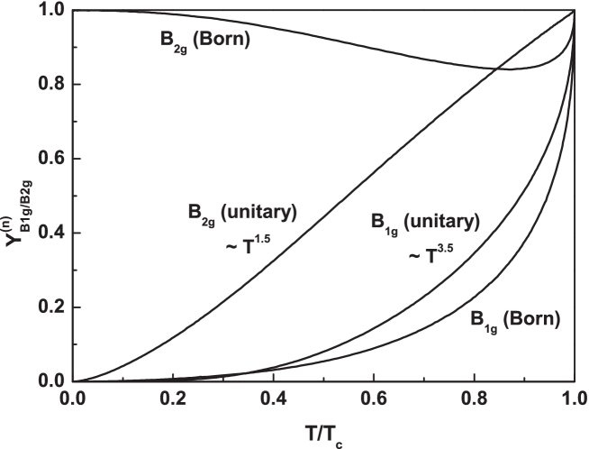
Figure 1: Temperature dependence of the generalized Yosida functions $Y^{(n)}_{aa}(T)$, characterizing the transport parameters $T_{aa}^{Q}$, for the Raman polarizations B_1g and B_2g in the unitary ($n=1$) and the Born ($n=3$) limit, as evaluated from Eq. (54) in the text. The stated power laws fit very well at intermediate temperatures. In the low temperature limit, even analytical expressions for $Y_{aa}^{(n)}(T)$ are found (c. f. Eqs. (62) and (63)).

which describe the temperature dependence of $T^{Q}_{aa}$. On the other hand, an inspection of (50) shows, that in the limit $E_{\bf k}\to 0$ the elastic relaxation time $\tau_{\bf k}^{\rm e}$ tends to a finite value in the unitary limit, which reflects existence of an impurity band originating from resonant pair–breaking processes, described by the t–matrix. This leads to a low–temperature offset in the temperature dependence of $T^{Q}_{aa}$, which is described by the dimensionless parameter

$$C_{aa}=\frac{\hbar}{2\tau_{\rm N}}\frac{1}{\langle a_{\bf p}^{2}\rangle_{\rm FS}}\left\langle\frac{a_{\bf p}^{2}\Sigma_{0}^{{\prime\prime}2}}{\left[\Sigma_{0}^{{\prime\prime}2}+\Delta_{\bf p}^{2}\right]^{3/2}}\right\rangle_{\rm FS}$$ (55)

For a $d$–wave gap of the form (2) the integrals over the Fermi surface can be performed in Eq. (55) in the unitary limit with the result:

$$C_{aa} = \frac{2}{\pi}\frac{\hbar}{\tau_{\rm N}\Delta_{0}}\frac{\Sigma_{0}^{\prime\prime}}{\Delta_{0}}\begin{cases}K\left(\frac{i\Delta_{0}}{\Sigma_{0}^{\prime\prime}}\right)-\frac{\Sigma_{0}^{\prime\prime 2}}{\Sigma_{0}^{\prime\prime 2}+\Delta_{0}^{2}}E\left(\frac{i\Delta_{0}}{\Sigma_{0}^{\prime\prime}}\right)\ \ ;\ \ {\rm B}_{1g}\cr\cr E\left(\frac{i\Delta_{0}}{\Sigma_{0}^{\prime\prime}}\right)-K\left(\frac{i\Delta_{0}}{\Sigma_{0}^{\prime\prime}}\right)\ \ \ \ \ \ \ \ \ \ \ \ ;\ \ {\rm B}_{2g}\end{cases}$$

$$\stackrel{{\scriptstyle\Sigma_{0}^{\prime\prime}\ll\Delta_{0}}}{{=}} \frac{2}{\pi}\frac{\hbar}{\tau_{\rm N}\Delta_{0}}\begin{cases}\left(\frac{\Sigma_{0}^{\prime\prime}}{\Delta_{0}}\right)^{2}\ln\frac{4\Delta_{0}}{\Sigma_{0}^{\prime\prime}}-\frac{\Sigma_{0}^{\prime\prime 2}}{\Sigma_{0}^{\prime\prime 2}+\Delta_{0}^{2}}\ \ ;\ \ {\rm B}_{1g}\cr\cr\ \ \ 1+\frac{\Sigma^{\prime\prime 2}_{0}}{2\Delta_{0}^{2}}\left[\frac{1}{2}-\ln\frac{4\Delta_{0}}{\Sigma^{\prime\prime}_{0}}\right]\ \ ;\ \ {\rm B}_{2g}\end{cases}$$

Here $K$ and $E$ refer to the complete elliptic integrals of first and second kind, respectively. The description of the transport parameter $T^{Q}_{aa}$ becomes exact at $T=0$ and represents a very accurate approximation just below the transition temperature. For intermediate temperatures, Eq. (53) represents a physically quite transparent temperature interpolation scheme, which, however, is meaningful only as long as the generalized Yosida functions $Y^{(n)}_{aa}$ vanish in the low temperature limit $T\to 0$. We turn now to an evaluation of Eq. (53) in the low temperature limit. In the limits of unitary ($\delta_{0}\to\pi/2$) and Born ($\delta_{0}\to 0$) scattering, we obtain for not too large values of $\Sigma^{\prime\prime}_{0}/\Delta_{0}$ (i. e. low impurity concentrations):

$$\lim_{T\to 0}T_{aa}^{\rm Q} \stackrel{{\scriptstyle\delta_{0}\to\pi/2}}{{=}} N_{\rm F}\langle a_{\bf p}^{2}\rangle_{\rm FS}\ \frac{2\hbar}{\pi\Delta_{0}}\cdot\begin{cases}\left(\frac{\Sigma^{\prime\prime}_{0}}{\Delta_{0}}\right)^{2}\ln\frac{4\Delta_{0}}{\Sigma^{\prime\prime}_{0}}\ \ ;\ \ {\rm B}_{1g}\cr\ \ \ \ \ \ \ \ \ 1\ \ \ \ \ \ \ \ ;\ \ {\rm B}_{2g}\end{cases}$$ (57)

$$\lim_{T\to 0}T_{aa}^{\rm Q} \stackrel{{\scriptstyle\delta_{0}\to 0}}{{=}} N_{\rm F}\langle a_{\bf p}^{2}\rangle_{\rm FS}\ \frac{2\hbar}{\pi\Delta_{0}}\cdot\begin{cases}\ \ \ \ 0\ \ \ ;\ \ {\rm B}_{1g}\cr\ \ \ \ 1\ \ ;\ \ \ {\rm B}_{2g}\end{cases}$$

This important result shows an amazing qualitative difference between the B_1g and the B_2g polarization: in the B_1g case, the transport parameter depends on the parameters $n_{i}$ and $\delta_{0}$, characterizing the impurity scattering, whereas in the B_2g case it does not. This behavior of the zero temperature transport properties in the B_2g case occurs also in the case of electronic conductivity[21], the electronic thermal conductivity [22], the (electron–phonon interaction induced) sound attenuation[23] and has been termed universal transport[21]. For the case of Raman scattering, this result has first been derived for the unitary limit in ref. [24].

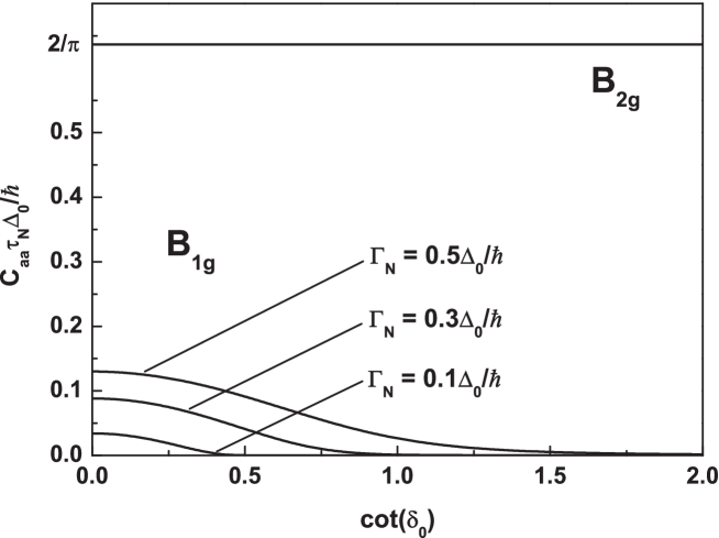
Figure 2: Normalized offset parameter $C_{aa}\tau_{\rm N}\propto T_{aa}^{Q}(T=0)$ giving rise to universal transport in the case of B_2g–symmetry ($\Gamma_{N}=1/\tau_{N}$).

For the numerical computations it is important to see that in the Born limit ($\delta_{0}\to 0$) there is a simple relation between $\Sigma^{\prime\prime}_{0}$ and the normal state lifetime $\tau_{\rm N}$, namely

$$\Sigma^{\prime\prime}_{0}=4\Delta_{0}\exp\left(-\frac{\pi\tau_{\rm N}\Delta_{0}}{\hbar}\right)$$ (58)

In the unitary limit, on the other hand, one has to solve the transcendental equation

$$\left(\frac{\Sigma_{0}^{\prime\prime}}{\Delta_{0}}\right)^{2}\ln\left(\frac{4\Delta_{0}}{\Sigma_{0}^{\prime\prime}}\right)=\frac{\pi\hbar}{4\tau_{\rm N}\Delta_{0}}$$ (59)

in order to relate $\Sigma^{\prime\prime}_{0}$ to $\tau_{\rm N}$. Defining $\gamma=\hbar/\tau_{\rm N}\Delta_{0}$, the solution of Eq. (59) can be expressed as

$$\Sigma_{0}^{\prime\prime}=\sqrt{\frac{\pi\gamma}{2\left|W_{-1}\left(\frac{\pi\gamma}{32}\right)\right|}}$$ (60)

with $W$ the Lambert–$W$ function, for which an expansion for small arguments reads [35]:

$$|W_{-1}(z)|=\ln\frac{1}{z}+\ln\left(\ln\frac{1}{z}\right)\left[1+\frac{1}{\ln\frac{1}{z}}\right]+\dots$$ (61)

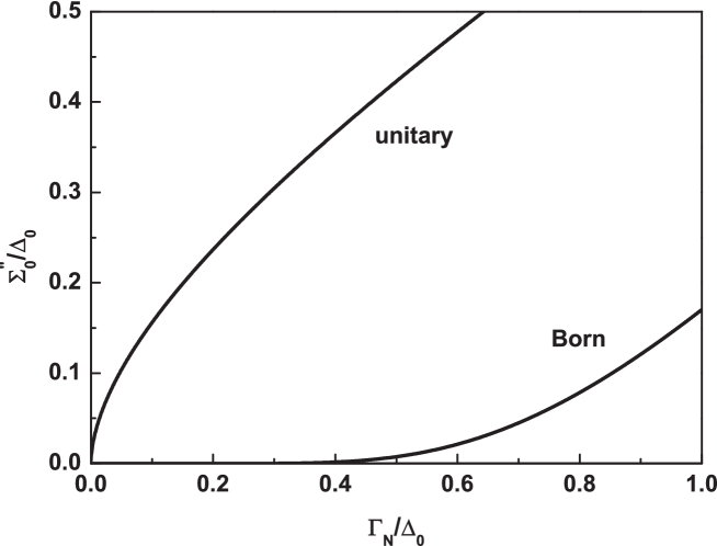
Figure 3: Normalized imaginary part of the impurity self energy $\Sigma^{\prime\prime}_{0}=\Im\Sigma_{e}(0)$ in the unitary and the Born limit as a function of the normalized scattering rate ${\Gamma_{N}=1/\tau_{N}}$.

We consider finally the temperature dependence of $T^{Q}_{aa}$ in the low temperature limit, where an analytical treatment is possible. Using the expansion of $D(x)=x[1+i(2/\pi)\ln(x/4)]$ for $x=E_{\bf k}/\Delta_{0}\ll 1$, one obtains in the B_1g case

$$\lim_{T\to 0}Y^{(1)}(T) = 4\left(\frac{k_{\rm B}T}{\Delta_{0}}\right)^{4}\left[b_{10}-b_{11}\ln\left(\frac{2\Delta_{0}}{k_{\rm B}T}\right)+b_{12}\ln^{2}\left(\frac{2\Delta_{0}}{k_{\rm B}T}\right)\right]$$ (62)

$$\lim_{T\to 0}Y^{(3)}(T) = \frac{1}{12}\left(\frac{\pi k_{\rm B}T}{\Delta_{0}}\right)^{2}$$

and in the B_2g case

$$\lim_{T\to 0}Y^{(1)}(T) = 4\left(\frac{k_{\rm B}T}{\Delta_{0}}\right)^{2}\left[b_{20}-b_{21}\ln\left(\frac{2\Delta_{0}}{k_{\rm B}T}\right)+b_{22}\ln^{2}\left(\frac{2\Delta_{0}}{k_{\rm B}T}\right)\right]$$ (63)

$$\lim_{T\to 0}Y^{(3)}(T) = 1$$

Here we have defined the coefficients

$$b_{k0} = a_{k0}+\frac{4a_{k2}}{\pi^{2}}$$

$$b_{k1} = \frac{a_{k1}}{\pi^{2}}$$ (64)

$$b_{k2} = \frac{4a_{k0}}{\pi^{2}}\ \ ;\ \ k=1,2$$

and

$$a_{k\mu}=\int_{0}^{\infty}dv\frac{v^{6-2k}\ln^{\mu}v}{\cosh^{2}v}$$ (65)

In Fig. 1 we have plotted the generalized Yosida functions $Y_{aa}^{(n)}(T)$, which characterize the temperature-dependence of the quasiparticle transport parameters $T_{aa}^{Q}$ vs. reduced temperature $T/T_{\rm c}$ [c. f. Eq. (52)]. Clearly, the theory predicts a temperature–independent result for $T^{Q}_{aa}$ in the B_2g case in the Born scattering limit. This was actually the motivation for Pethick and Pines[17] to apply the t–matrix to the description of transport in heavy Fermion superconductors, since the experiments showed transport parameters vanishing at low $T$ instead of staying constant below $T_{\rm c}$. It is quite amazing, that the $T$–dependence of $Y^{(1)}_{aa}(T)$ is close to the power laws $T^{3.5}$ in the B_1g– and $T^{1.5}$ in the B_2g–case, as predicted by Moreno and Coleman for the ultrasound attenuation[26]. In Fig. 2 we have plotted the normalized parameters $C_{aa}\tau_{\rm N}$, which are proportional to $T_{aa}^{Q}(0)$, vs. $s$–wave scattering phase shift $\cot\delta_{0}$ for $B_{1g}$ ($a_{\bf p}=\cos(2\phi)$) and $B_{2g}$ ($a_{\bf p}=\sin(2\phi)$) symmetry. These parameters characterize the low–$T$ offset in the $T$–dependence of the transport parameters according to Eq. (52). A strong dependence of these offsets on $\delta_{0}$ and $\hbar\Delta_{0}/\tau_{\rm N}$ is seen in the B_1g case, whereas in the B_2g case $T_{aa}^{Q}(T\to 0)$ is independent of $\delta_{0}$ and $\hbar\Delta_{0}/\tau_{\rm N}$, at least in the limit of low impurity concentrations $\hbar\Delta_{0}/\tau_{\rm N}\to 0$. In Fig. 3 we have plotted the dependence of the quantity $\Sigma_{0}^{\prime\prime}/\Delta_{0}$, which enters the low–$T$ offset parameter $C_{aa}$ in Eq. (53), as a function of the normalized normal state scattering rate $\Gamma_{\rm N}/\Delta_{0}$ for both the unitary and the Born limit of quasiparticle scattering.

9 Raman quasiparticle transport and sound attenuation

In this section we would like to apply the results obtained in section 8 to the transport parameters connected with the attenuation of ultrasound and Raman scattering, and discuss strong similarities in their polarization dependence. The vertex function $a_{\bf p}$ reads in these two cases for dimension $d$:

$$a_{\bf p}=\begin{cases}\hat{\sigma}_{\bf p}\equiv p_{\rm F}v_{\rm F}\left[(\hat{\bf p}\cdot\hat{\bf q})(\hat{\bf p}\cdot\hat{\bf u})-\frac{1}{d}\hat{\bf q}\cdot\hat{\bf u}\right]\ \ ;\ \ \ {\rm sound\ attenuation}\cr\ \ \ \ \ \ \ \ \gamma_{\bf p}\equiv m\hat{{\bf e}}_{I}\cdot{\bf M}_{\bf p}^{-1}\cdot\hat{{\bf e}}_{S}\ \ \ \ \ \ \ \ \ \ \ \ ;\ \ {\rm Raman}\end{cases}$$ (66)

Here the unit vectors $\hat{\bf q}$ and $\hat{\bf u}$ refer to the sound propagation and polarization directions, respectively, whereas $\hat{\bf e}_{I,S}$ denote the polarizations of the incoming and reflected photon in an electronic Raman scattering process. Without limiting generality, we may assume

$$\hat{\bf q},\hat{{\bf e}}_{I} = \left(\begin{array}[]{c}\cos\alpha\cr\sin\alpha\end{array}\right)$$ (69)

$$\hat{\bf u},\hat{{\bf e}}_{S} = \left(\begin{array}[]{c}\cos\beta\cr\sin\beta\end{array}\right)$$ (72)

With this 2–$d$ representation, the stress tensor vertex and the Raman vertex assume the form

$$\hat{\sigma}_{\bf p} = \frac{p_{\rm F}v_{\rm F}}{2}\left\{\cos(\alpha+\beta)\Phi_{\bf p}^{B_{1g}}+\sin(\alpha+\beta)\Phi_{\bf p}^{B_{2g}}\right\}$$ (73)

$$\gamma_{\bf p} = \cos(\alpha-\beta)\left[{\rm const}+\gamma_{0}^{A_{1g}}\Phi_{\bf p}^{A_{1g}}\right]+\cos(\alpha+\beta)\gamma_{0}^{B_{1g}}\Phi_{\bf p}^{B_{1g}}+\sin(\alpha+\beta)\gamma_{0}^{B_{2g}}\Phi_{\bf p}^{B_{2g}}$$

In (68) the quantities $\gamma_{0}$ are constants which depend on the band structure and the functions $\Phi_{\bf p}$ denote the relevant harmonics of the Fermi surface[27]. In the simplest case of a cylindrical Fermi surface one may write

$$\Phi_{\bf p}^{A_{1g}}=\cos(4\phi)\ \ ;\ \ \Phi_{\bf p}^{B_{1g}}=\cos(2\phi)\ \ ;\ \ \Phi_{\bf p}^{B_{2g}}=\sin(2\phi)$$ (74)

Note that since by definition $\left\langle\hat{\sigma}_{\bf p}\right\rangle_{\rm FS}=0$, the stress tensor vertex function does not have a contribution from the A_1g basis function. In other respects, this appears to be the only difference between Raman and stress tensor vertex. Note that in particular the dependence of the transport parameters on the directions $(\hat{\bf q}$, $\hat{\bf u})$ and ($\hat{{\bf e}}_{I}$, $\hat{{\bf e}}_{S}$) is the same. With $\hat{\bf x}^{\prime}=(\hat{\bf x}+\hat{\bf y})/\sqrt{2}$ and $\hat{\bf y}^{\prime}=(\hat{\bf x}-\hat{\bf y})/\sqrt{2}$, this means that the attenuation of transverse sound propagating in the $\hat{\bf x}$– ($\hat{\bf x}^{\prime}$–) direction corresponds to the $\hat{\bf x}\hat{\bf y}$– ($\hat{\bf x}^{\prime}\hat{\bf y}^{\prime}$–) Raman polarization coupling to the B_2g– (B_1g–) basis functions. The attenuation of longitudinal sound, on the other hand, propagating in the $\hat{\bf x}$– ($\hat{\bf x}^{\prime}$–) direction, corresponds to the $\hat{\bf x}\hat{\bf x}$– ($\hat{\bf x}^{\prime}\hat{\bf x}^{\prime}$–) Raman polarization and hence to the combinations A_1g+B_1g (A_1g+B_2g) respectively[27]. We proceed now to write down the transport parameters associated with sound attenuation and electronic Raman scattering. In order to be able to compare these transport phenomena, we therefore limit the following considerations entirely to the B_1g and B_2g basis functions and define generalized Yosida functions (c. f. Eq. (54))

$$Y^{(n)}_{s}(T) = \frac{1}{\langle(\Phi^{s}_{\bf p})^{2}\rangle_{\rm FS}}\left\langle 2\int\limits_{\Delta_{\bf p}}^{\infty}dE_{\bf p}\frac{\sqrt{E_{\bf p}^{2}-\Delta_{\bf p}^{2}}}{E_{\bf p}}\frac{|D(E_{\bf p})|^{3-n}}{\Re D(E_{\bf p})}y_{\bf p}(\Phi^{s}_{\bf p})^{2}\right\rangle_{\rm FS}$$ (75)

$$s = {\rm B}_{1g},{\rm B}_{2g}$$

and the dimensionless (offset) parameters (c. f. Eq. (55))

$$C_{s}=\frac{\hbar}{2\tau_{\rm N}}\frac{1}{\langle(\Phi^{s}_{\bf p})^{2}\rangle_{\rm FS}}\left\langle\frac{(\Phi^{s}_{\bf p})^{2}\Sigma_{0}^{{\prime\prime}2}}{\left[\Sigma_{0}^{{\prime\prime}2}+\Delta_{\bf p}^{2}\right]^{3/2}}\right\rangle_{\rm FS}\ \ ;\ \ s={\rm B}_{1g},{\rm B}_{2g}$$ (76)

Let us start with the sound attenuation, which can be described by the wavenumber $\alpha(\omega)$[36]:

$$\alpha(\omega)=\frac{\omega^{2}}{\rho c_{\rm s}^{3}}\bar{\eta}$$ (77)

Here $\bar{\eta}$ is a viscous dissipation parameter, which has the following form

$$\bar{\eta}(T) = \eta_{\rm N}p_{s}(\alpha,\beta)\begin{cases}C_{s}+(1-C_{s})Y_{s}^{(1)}(T)\ \ ;\ \ {\rm unitary\ limit}\cr\ \ \ \ \ \ \ \ Y_{s}^{(3)}(T)\ \ \ \ \ \ \ \ \ \ \ \ ;\ \ {\rm Born\ limit}\end{cases}$$ (78)

$$p_{s}(\alpha,\beta) = \cos^{2}(\alpha+\beta)\delta_{s,{\rm B}_{1g}}+\sin^{2}(\alpha+\beta)\delta_{s,{\rm B}_{2g}}$$

$$\eta_{\rm N} = \frac{1}{4}np_{\rm F}v_{\rm F}\tau_{\rm N}$$

In (73) $\eta_{\rm N}$ denotes the impurity–limited normal state viscosity. The Raman case, on the other hand, is characterized by a transport parameter which is reminiscent of the second viscosity, discussed in section 6, generalized to include the square of the Raman vertex in the Fermi surface average:

$$T^{Q}_{\gamma\gamma}(T)=\zeta_{\gamma\gamma}^{(3)}(T)$$ (79)

$\zeta_{\gamma\gamma}^{(3)}$ has the form

$$\zeta_{\gamma\gamma}^{(3)}(T) = \zeta_{\gamma\gamma}^{(3){\rm N}}\left(\gamma_{0}^{s}\right)^{2}p_{s}(\alpha,\beta)\begin{cases}C_{s}+(1-C_{s})Y_{s}^{(1)}(T)\ \ ;\ \ {\rm unitary\ limit}\cr\ \ \ \ \ \ \ \ Y_{s}^{(3)}(T)\ \ \ \ \ \ \ \ \ \ \ \ ;\ \ {\rm Born\ limit}\end{cases}$$ (80)

$$\zeta_{\gamma\gamma}^{(3){\rm N}} = N_{\rm F}\tau_{\rm N}$$

Hence we have demonstrated the physical similarity of the hydrodynamic transport parameters emerging from the electronic Raman effect and the sound attenuation in $d$=2.

10 Conclusion

In summary, we have demonstrated, how the response and transport properties of unconventional superconductors are linked together in a very simple way, if the long wavelength limit ${\bf q}\to 0$ is taken. In this limit the contributions of the normal component (the BQP system) and the condensate (the system of Cooper pairs) to the response and transport simply add up and allow for a two–fluid description which is valid at arbitrary quasiclassical frequencies. The result for the quasiparticle transport parameters $T_{aa}^{Q(0)}$ and $T_{aa}^{Q}$ are qualitatively different before and after the renormalization of the response with respect to the long–range Coulomb interaction. These transport parameters can be represented in a form, which is valid both in the limits of weak (Born) and strong (unitary) scattering and which makes their dependence on temperature and the impurity scattering parameters ($n_{i},\delta_{0}$) particularly clear. In the low $T$ limit, the temperature dependence can be evaluated analytically and is found to differ from a simple power–law behavior, predicted earlier [29]. In the limit of Born scattering, some components of the quasiparticle transport tensors stay constant in the low $T$ limit and thus exclude the possibility of weak scattering as a model for impurity limited transport for example in the cuprate superconductors. In the unitary limit, on the other hand, we find offsets in the transport parameters, which, in certain cases, do not depend on the impurity scattering parameters. This so–called universal transport occurs in both the impurity–limited electronic Raman effect and the attenuation of ultrasound. We could finally demonstrate, that for quasi–2–$d$ systems the Raman scattering intensity is closely related to the transport of momentum (stress tensor) in the BQP system.

Appendix: Response and relaxation of densities and currents

In this appendix we would like to demonstrate that although one has to carefully distinguish the response of quasiparticle densities and currents (their reactive response is indeed different) their dissipative response, characterized by their transport parameters, is the same. This justifies the line of arguments presented in section 5 of this paper. We now give a more general derivation of response functions and transport parameters for a system of Bogoliubov quasiparticles (BQP) in $d$–wave superconductors. The dynamics of such a BQP system is governed by a scalar kinetic equation for the distribution function $\delta\nu_{\bf k}({\bf q},\omega)$ (c. f. Eq. (21) in the text):

$$\omega\delta\nu_{\bf k}-{\bf q}\cdot{\bf V}_{\bf k}h_{\bf k} = i\delta I_{\bf k}$$ (81)

Here ${\bf V}_{\bf k}=\partial E_{\bf k}/\hbar\partial{\bf k}=(\xi_{\bf k}/E_{\bf k}){\bf v}_{\bf k}$ is the BQP group velocity and the distribution function

$$h_{\bf k}=\delta\nu_{\bf k}+y_{\bf k}\delta E_{\bf k}$$ (82)

describes the deviation from local equilibrium. In (76) $\delta I_{\bf k}$ is the collision integral, which is assumed to be limited to the case of purely elastic scattering and to have therefore the following (quasiparticle number conserving) form

$$\delta I_{\bf k} = \delta I_{\bf k}^{(+)}+\delta I_{\bf k}^{(-)}$$

$$\delta I_{\bf k}^{(+)} = -\frac{h_{\bf k}^{(+)}}{\tau_{\bf k}^{\rm e}}+\frac{\xi_{\bf k}}{E_{\bf k}}\frac{y_{\bf k}}{\tau_{\bf k}^{\rm e}}\frac{\left\langle\frac{\xi_{\bf p}}{E_{\bf p}}\frac{h_{\bf p}^{(+)}}{\tau_{\bf p}^{\rm e}}\right\rangle}{\left\langle\frac{\xi_{\bf p}^{2}}{E_{\bf p}^{2}}\frac{y_{\bf p}}{\tau_{\bf p}^{\rm e}}\right\rangle}$$ (83)

$$\delta I_{\bf k}^{(-)} = -\frac{h_{\bf k}^{(-)}}{\tau_{\bf k}^{\rm e}}\ \ ;\ \ \left\langle\dots\right\rangle=\frac{1}{V}\sum_{{\bf p}\sigma}\dots$$

Here the index $\pm$ denotes the parity of the distribution function $h_{\bf k}$ with respect to the operation ${\bf k}\to-{\bf k}$. The first part (+) of the collision integral describes the conservation of the BQP density, whereas the second part (–) describes the relaxation of the BQP current, here, for simplicity, treated within a simple relaxation time approximation. At this stage it is important to decompose the BQP energy change $\delta E_{\bf k}$ into even and odd contibutions w. r. t. the operation ${\bf k}\to-{\bf k}$:

$$\delta E_{\bf k} = a_{\bf k}\left[\frac{\xi_{\bf k}}{E_{\bf k}}\delta\xi_{a}+{\bf v}_{\bf k}\cdot\delta{\mbox{\boldmath$\zeta$}}_{a}\right]$$ (84)

In (79) the quantity $\delta{\mbox{\boldmath$\zeta$}}_{a}$ denotes a generalized vector potential. Note that in the case of the electromagnetic response ($a_{\bf k}\equiv e$) one has $\delta\xi_{a}=\Phi$ and $\delta{\mbox{\boldmath$\zeta$}}_{a}=-{\bf A}/c$. The macroscopic BQP density is defined through (c. f. Eq. (21) in the text):

$$\delta n_{a}^{Q}=\left\langle a_{\bf p}\frac{\xi_{\bf p}}{E_{\bf p}}\delta\nu_{\bf p}\right\rangle$$ (85)

Using this definition, one may derive from (76) the following relaxation equation for $\delta n_{a}^{Q}$:

$$\omega\delta n_{a}^{Q}-{\bf q}\cdot{\bf j}_{a}^{Q}=i\left\langle a_{\bf p}\frac{\xi_{\bf p}}{E_{\bf p}}\delta I_{\bf p}^{(+)}\right\rangle$$ (86)

Here we may identify the BQP current ${\bf j}_{a}^{Q}$ in the form

$${\bf j}_{a}^{Q} = \left\langle a_{\bf p}\frac{\xi_{\bf p}}{E_{\bf p}}{\bf V}_{\bf p}h_{\bf p}^{(-)}\right\rangle=\left\langle a_{\bf p}\frac{\xi_{\bf p}^{2}}{E_{\bf p}^{2}}{\bf v}_{\bf p}h_{\bf p}^{(-)}\right\rangle$$ (87)

In the case $\langle a_{\bf p}\rangle_{\rm FS}=0$, the solution of the kinetic equation for the BQP density $\delta n_{a}^{Q}$, discussed in the text, reads after invoking the effects of the long–range Coulomb interaction (c. f. Eq. (24))

$$\delta n_{a}^{Q} = \chi_{aa}^{Q}(\omega)\delta\xi_{a}\ \ ;\ \ \chi_{aa}^{Q}(\omega)=-\left\langle a_{\bf p}^{2}\frac{\xi_{\bf p}^{2}}{E_{\bf p}^{2}}\frac{y_{\bf p}}{1-i\omega\tau_{\bf p}^{\rm e}}\right\rangle$$ (88)

We wish now to write down the corresponding solution for the generalized current ${\bf j}_{a}^{Q}$. From (76) one finds for the distribution function $h_{\bf k}^{(-)}$

$$h_{\bf k}^{(-)} = \frac{-i\omega\tau_{\bf k}^{\rm e}}{1-i\omega\tau_{\bf k}^{\rm e}}y_{\bf k}\delta E_{\bf k}^{(-)}-\frac{i{\bf q}\cdot{\bf V}_{\bf k}\tau_{\bf k}^{\rm e}}{1-i\omega\tau_{\bf k}^{\rm e}}h_{\bf k}^{(+)}$$ (89)

In the long wavelength limit ${\bf q}\to 0$ this result, inserted into (82) leads to

$${\bf j}_{a}^{Q} = {\bf X}_{aa}^{Q}(\omega)\cdot\delta{\mbox{\boldmath$\zeta$}}_{a}\ \ ;\ \ {\bf X}_{aa}^{Q}(\omega)=\left\langle a_{\bf p}^{2}\frac{\xi_{\bf p}^{2}}{E_{\bf p}^{2}}{\bf v}_{\bf p}:{\bf v}_{\bf p}\frac{-i\omega\tau_{\bf p}^{\rm e}}{1-i\omega\tau_{\bf p}^{\rm e}}y_{\bf p}\right\rangle$$ (90)

One immediately recognizes that the response functions for the BQP density $\chi_{aa}^{Q}(\omega)$ and the quasiparticle current ${\bf X}_{aa}^{Q}(\omega)$ differ, besides the tensor structure of the latter, in the usual way in their dependence on the dimensionless quantity $\omega\tau_{\bf p}^{\rm e}$. It is instructive to decompose the density response function $\chi_{aa}^{Q}$ into its real and imaginary parts, respectively:

$$\chi_{aa}^{Q} = \chi_{aa}^{Q\prime}+i\chi_{aa}^{Q\prime\prime}$$

$$\chi_{aa}^{Q\prime} = -\left\langle a_{\bf p}^{2}\frac{\xi_{\bf p}^{2}}{E_{\bf p}^{2}}\frac{y_{\bf p}}{1+(\omega\tau_{\bf p}^{\rm e})^{2}}\right\rangle$$ (91)

$$\chi_{aa}^{Q\prime\prime} = -\omega\left\langle a_{\bf p}^{2}\frac{\xi_{\bf p}^{2}}{E_{\bf p}^{2}}\frac{y_{\bf p}\tau_{\bf p}^{\rm e}}{1+(\omega\tau_{\bf p}^{\rm e})^{2}}\right\rangle\equiv-\omega T_{aa}^{Q}$$

In the same way we obtain for ${\bf X}_{aa}^{Q}$:

$${\bf X}_{aa}^{Q} = {\bf X}_{aa}^{Q\prime}+i{\bf X}_{aa}^{Q\prime\prime}$$

$${\bf X}_{aa}^{Q\prime} = \left\langle a_{\bf p}^{2}\frac{\xi_{\bf p}^{2}}{E_{\bf p}^{2}}{\bf v}_{\bf p}:{\bf v}_{\bf p}\frac{y_{\bf p}(\omega\tau_{\bf p}^{\rm e})^{2}}{1+(\omega\tau_{\bf p}^{\rm e})^{2}}\right\rangle$$ (92)

$${\bf X}_{aa}^{Q\prime\prime} = -\omega\left\langle a_{\bf p}^{2}\frac{\xi_{\bf p}^{2}}{E_{\bf p}^{2}}{\bf v}_{\bf p}:{\bf v}_{\bf p}\frac{y_{\bf p}\tau_{\bf p}^{\rm e}}{1+(\omega\tau_{\bf p}^{\rm e})^{2}}\right\rangle\equiv-\omega{\bf T}_{aa}^{Q}$$

It is interesting to formally compare the response of the BQP density and current in the following way: The density response can be written in terms of an effective BQP relaxation time $\tau_{aa}^{Q}$ in the form (c. f. Eq. (33) in the text):

$$\delta n_{a}^{Q} = -\frac{\left\langle a_{\bf p}^{2}\frac{\xi_{\bf p}^{2}}{E_{\bf p}^{2}}y_{\bf p}\right\rangle}{1-i\omega\tau_{aa}^{Q}}\delta\xi_{a}\ \ ;\ \ \tau_{aa}^{Q}=\frac{\left\langle a_{\bf p}^{2}\frac{\xi_{\bf p}^{2}}{E_{\bf p}^{2}}\frac{y_{\bf p}\tau_{\bf p}^{\rm e}}{1-i\omega\tau_{\bf p}^{\rm e}}\right\rangle}{\left\langle a_{\bf p}^{2}\frac{\xi_{\bf p}^{2}}{E_{\bf p}^{2}}\frac{y_{\bf p}}{1-i\omega\tau_{\bf p}^{\rm e}}\right\rangle}$$ (93)

whereas the current obeys a Drude–like law, involving a corresponding effective current relaxation time $\tau_{avav}^{Q}$:

$${\bf j}_{a}^{Q} = \frac{-i\omega\tau_{avav}^{Q}}{1-i\omega\tau_{avav}^{Q}}\left\langle a_{\bf p}^{2}{\bf v}_{\bf p}\frac{\xi_{\bf p}^{2}}{E_{\bf p}^{2}}y_{\bf p}({\bf v}_{\bf p}\cdot\delta{\mbox{\boldmath$\zeta$}}_{a})\right\rangle\ \ ;\ \ \tau_{avav}^{Q}=\frac{\left\langle(a_{\bf p}{\bf v}_{\bf p})^{2}\frac{\xi_{\bf p}^{2}}{E_{\bf p}^{2}}\frac{y_{\bf p}\tau_{\bf p}^{\rm e}}{1-i\omega\tau_{\bf p}^{\rm e}}\right\rangle}{\left\langle(a_{\bf p}{\bf v}_{\bf p})^{2}\frac{\xi_{\bf p}^{2}}{E_{\bf p}^{2}}\frac{y_{\bf p}}{1-i\omega\tau_{\bf p}^{\rm e}}\right\rangle}$$ (94)

Eqs. (88) and (89) are clearly seen to describe the formal difference between the density and current response: whereas the effective relaxation times for the densities and currents differ only by the use of different vertices $a_{\bf p}\leftrightarrow a_{\bf p}{\bf v}_{\bf p}$, the response of the current is Drude–like, whereas the response of the density is not. Nevertheless we have now arrived at a stage where we can analyze the connection between the density and current response functions and the transport parameters associated with the densities and currents. Defining generalized forces

$$f_{a} = -i\omega\delta\xi_{a}\ \ ;\ \ {\bf f}_{a}=-i\omega\delta{\mbox{\boldmath$\zeta$}}_{a}$$ (95)

we may write

$$\delta n_{a}^{Q} = \chi_{aa}^{Q\prime}\delta\xi_{a}+T_{aa}^{Q}f_{a}$$ (96)

$${\bf j}_{a}^{Q} = {\bf X}_{aa}^{Q\prime}\cdot\delta{\mbox{\boldmath$\zeta$}}_{a}+{\bf T}_{aa}^{Q}\cdot{\bf f}_{a}$$

An inspection of Eqs. (83, 85, 88, 89) shows that while the reactive response of BQP densities and currents is qualitatively different, the dissipative response of densities and currents, represented by the transport parameters $T_{aa}^{Q}$ and ${\bf T}_{aa}^{Q}$ is similar in structure, if on makes the replacements for the vertices $a_{\bf p}\to a_{\bf p}{\bf v}_{\bf p}$. The transport parameters $T_{aa}^{Q}$ and ${\bf T}_{aa}^{Q}$ read

$$T_{aa}^{Q}(\omega) = -\frac{\chi_{aa}^{Q\prime\prime}(\omega)}{\omega}=\left\langle a_{\bf p}^{2}\frac{\xi_{\bf p}^{2}}{E_{\bf p}^{2}}\frac{y_{\bf p}\tau_{\bf p}^{\rm e}}{1+(\omega\tau_{\bf p}^{\rm e})^{2}}\right\rangle$$ (97)

$${\bf T}_{aa}^{Q}(\omega) = -\frac{{\bf X}_{aa}^{Q\prime\prime}(\omega)}{\omega}=\left\langle a_{\bf p}^{2}\frac{\xi_{\bf p}^{2}}{E_{\bf p}^{2}}{\bf v}_{\bf p}:{\bf v}_{\bf p}\frac{y_{\bf p}\tau_{\bf p}^{\rm e}}{1+(\omega\tau_{\bf p}^{\rm e})^{2}}\right\rangle$$

Hence we have arrived at a unified description of transport phenomena associated with the Raman and stress tensor response and have therefore justified the argumentation presented in section 5.

References

• [1] D. D. Osheroff, D. M. Lee, and R. C. Richardson, Phys. Rev. Lett. 29, 920 (1972).
• [2] for a theoretical review see: A. J. Leggett, Rev. Mod. Phys. 47, 331 (1975).
• [3] for an experimental review see: J. C. Wheatley, Rev. Mod. Phys. 47, 415 (1976).
• [4] for a comprehensive theoretical treatment see the book by: D. Vollhardt and P. Wölfle, The Superfluid Phases of Helium 3, Taylor and Francis, London, 1990.
• [5] CeCu2Si2: F. Steglich, J. Aarts, C. D. Bredl, W. Lieke, D. Meschede, W. Franz, and J. Schäfer, Phys. Rev. Lett. 43, 1892 (1979).
• [6] UBe13: H.–R. Ott, H. Rudigier, Z. Fisk, and J. L. Smith, Phys. Rev. Lett. 50, 1595 (1983).
• [7] UPt3: G. Stewart, Z. Fisk, J. O. Willis, and J. L. Smith, Phys. Rev. Lett. 52, 679 (1984).
• [8] J. G. Bednorz and K. A. Müller, Z. Phys. B64 189 (1986).
• [9] For a review see:
C. C. Tsuei and J. R. Kirtley, Rev. Mod. Phys. 72, 969 (2000).
• [10] Y. Maeno, H. Hashimoto, K. Yoshida, S. Nishizaki, T. Fujita, J. G. Bednorz, and F. Lichtenberg, Nature 372, 532 (1984).
• [11] D. Einzel, J Low Temp. Phys. 131, 1 (2003).
• [12] D. Einzel and J. M. Parpia, Phys. Rev. B 72, 214518 (2005).
• [13] For a recent review see:
T. P. Devereaux and R. Hackl, Rev. Mod. Phys. 79, 175 (2007) and references therein.
• [14] L. J. Buchholtz and G. Zwicknagl, Phys. Rev. 23, 5788 (1981).
• [15] D. Einzel and J. M. Parpia, J. Low Temp. Phys. 109, 1 (1997).
• [16] A. I. Golov, D. Einzel, G. Lawes, K. Matsumoto, and J. M. Parpia, Phys. Rev. Lett. 92, 195301–1 (2004).
• [17] C. J. Pethick and D. Pines, Phys. Rev. Lett. 57, 118 (1986).
• [18] P. Hirschfeld, D. Vollhardt and P. Wölfle, Solid State Comm. 59, 111 (1986).
• [19] For a recent review see:
A. V. Balatsky, I. Vekhter and Jian-Xin Zhu, Rev. Mod. Phys. 78, 373 (2006).
• [20] P. Hirschfeld, P. Wölfle, J. A. Sauls, , D. Einzel and W. O. Puttika, Phys. Rev. 40, 6695 (1989).
• [21] P. A. Lee, Phys. Rev. Lett. 71, 1887 (1993).
• [22] M. J. Graf, S.–K. Yip, J. A. Sausls and D. Rainer, Phys. Rev. B 53, 15147 (1996).
• [23] M. B. Walker, M. F. Smith and K. V. Samokhin, Phys. Rev. B 65, 014517-1 (2001).
• [24] W. C. Wu and J. P. Carbotte, Phys. Rev. B 57, R5614 (1998); for a review see ref. [28].
• [25] H. Monien, K. Scharnberg and D. Walker, Physica 148 B, 45 (1987).
• [26] J. Moreno and P. Coleman, Phys. Rev. B 53, R2995 (1996-II).
• [27] D. Einzel and R. Hackl, J. Raman Sectroscopy 27, 307 (1996).
• [28] T. P. Devereaux and A. P. Kampf, Int. J. of Modern Physics B 11, 2093 (1997).
• [29] T. P. Devereaux and D. Einzel, Phys. Rev. B 51, 16336 (1995).
• [30] P. Wölfle and D. Einzel, J. Low Temp. Phys. 23, 39 (1978).
• [31] Transport Phenomena, H. Smith and H. Hojgaard Jensen, Clarendon Press, Oxford (1989).
• [32] D. Einzel and D. Manske, Phys. Rev. B 70, 172507 (2004).
• [33] Ludwig Klam, Diploma thesis, unpublished (2006).
• [34] B. Arfi and C. J. Pethick, Phys. Rev. B 38, 2312 (1988).
• [35] R. M. Corless, G. H. Gonnet, D. E. G. Hare, D. J. Jeffrey, and D. E. Knuth, Advances in Computational Mathematics 5 4, 329 (1996) and references therein.
• [36] J. P. Rodriguez, Phys. Rev. Lett. 55, 250 (1985).