Evaluation of the semiclassical coherent state propagator in the presence of phase space caustics

Abstract

A uniform approximation for the coherent state propagator, valid in the vicinity of phase space caustics, was recently obtained using the Maslov method combined with a dual representation for coherent states. In this paper we review the derivation of this formula and apply it to two model systems: the one-dimensional quartic oscillator and a two-dimensional chaotic system.

1 Introduction

The representation of coherent states has been used to describe a wide variety of physical systems [1]. In particular, coherent states provide a natural phase space representation of quantum mechanics and are specially well suited to the study of the semiclassical limit. The coherent state representation was first formalized by Bargmann in 1961 [2] and later used by Glauber [3] to describe the electromagnetic field in quantum electrodynamics. Fairly complete review articles on coherent states and applications can be found in references [1, 4, 5].

The quantum propagator $K(z^{\prime\prime*},z^{\prime},T)\equiv\langle z^{\prime\prime}|e^{-i\hat{H}T/\hbar}|z^{\prime}\rangle$ represents the probability amplitude that an initial coherent state $|z^{\prime}\rangle$ evolves into another coherent state $|z^{\prime\prime}\rangle$ after a time $T$. A path integral formulation for this propagator was introduced by Klauder [6]. The paths contributing to $K(z^{\prime\prime*},z^{\prime},T)$ are those connecting $(q^{\prime},p^{\prime})\equiv(\langle z^{\prime}|\hat{q}|z^{\prime}\rangle,\langle z^{\prime}|\hat{p}|z^{\prime}\rangle)$ to $(q^{\prime\prime},p^{\prime\prime})\equiv(\langle z^{\prime\prime}|\hat{q}|z^{\prime\prime}\rangle,\langle z^{\prime\prime}|\hat{p}|z^{\prime\prime}\rangle)$. In the semiclassical limit, it turns out that the most important paths are complex classical trajectories governed by the hamiltonian function $\tilde{H}\equiv\langle z|\hat{H}|z\rangle$, with boundary conditions involving the average values $q^{\prime}$, $p^{\prime}$, $q^{\prime\prime}$ and $p^{\prime\prime}$. Klauder was the first to consider this type of approximation [7], being followed by a number of other contributors [8, 9, 10]. More recently, a detailed derivation of the semiclassical coherent state propagator for one dimensional systems was published [11]. In the last two decades much numerical and analytical work has been done in semiclassical methods with coherent states for one [12, 13, 14, 15, 16, 17, 18, 19] and two [20, 21] dimensional systems. A recent review can be found in reference [22].

While the semiclassical propagator is usually very accurate for short times, phase space caustics and non-contributing trajectories inevitably appear as $T$ increases, introducing large errors and imperfections [12, 13, 16, 20, 21]. Non-contributing trajectories must be identified and excluded from the calculation because their contributions to the propagator are non-physical. From the mathematical point of view, non-contributing trajectories correspond to forbidden deformations of the contour of integration necessary to carry out the stationary phase approximation that leads to the semiclassical formula. Phase space caustics, on the other hand, are special points where the amplitude of the semiclassical propagator diverges and the approximation simply breaks down. In order to calculate the propagator in the vicinity of caustics one needs to improve the semiclassical approximation, going beyond the usual quadratic expansion.

In two recent papers [23, 24] we have derived a uniform approximation for the coherent state propagator that remains finite in the presence of phase space caustics. The derivation involved the introduction of a dual representation for the coherent states and the method of Maslov [25]. In the present article, we review the formalism used in these previous papers and apply it to the one-dimensional quartic oscillator and to the two dimensional chaotic Nelson potential. We show that the uniform formula completely eliminates the divergences caused by the caustics, providing a very accurate semiclassical description of the propagator in these regions.

This paper is organized as follows: in the next section we briefly review the representation of coherent states and the quantum propagator. Section 3 describes the semiclassical approximation to the propagator based on a second order expansion around stationary trajectories. The dual representation for coherent states is introduced in section 4 and used in section 5 to derive the uniform approximation. In sections 6 and 7 we present numerical applications of the uniform formula and, in section 8, we present our final remarks.

2 The coherent state propagator

Let $H_{0}=\hbar\omega(\hat{a}^{\dagger}\hat{a}+1/2)$ be the Hamiltonian of a harmonic oscillator of mass $m$ and frequency $\omega$. The normalized coherent states of $H_{0}$ are defined by [1, 4, 5]

$$|z\rangle=e^{-\frac{1}{2}|z|^{2}}e^{z\,\hat{a}^{\dagger}}|0\rangle,$$ (1)

where

$$\hat{a}=\frac{1}{\sqrt{2}}\left(\frac{\hat{q}}{b}+i\frac{\hat{p}}{c}\right)\;,\quad\quad z=\frac{1}{\sqrt{2}}\left(\frac{q}{b}+i\frac{p}{c}\right)$$ (2)

and $|0\rangle$ is the oscillator’s ground state. The real labels $q$ and $p$ are the average values of the position and momentum operators respectively and the length scales $b=\sqrt{\hbar/(m\omega)}$ and $c=\sqrt{m\hbar\omega}$ satisfy $b\,c=\hbar$. Three important properties of the coherent states are (over)completeness, overlap relation and eigenvalue equation:

$$\mathbf{1}=\int|z\rangle\frac{d^{2}z}{\pi}\langle z|=\int|z\rangle\frac{dq\,dp}{2\pi\hbar}\langle z|~{},$$ (3)

$${\langle z_{i}|z_{j}\rangle=\exp{\{-\frac{1}{2}|z_{i}|^{2}+z_{i}^{*}z_{j}-\frac{1}{2}|z_{j}|^{2}}\}}$$ (4)

and

$$\hat{a}|z\rangle=z|z\rangle.$$ (5)

It will also be important in the derivation of our uniform approximation to define non-normalized coherent states, or Bargmann states [2], by

$$|z)=e^{z\,\hat{a}^{\dagger}}|0\rangle.$$ (6)

For these states the unit operator and the overlap equation become

$$\mathbf{1}=\int|z)\frac{e^{-|z|^{2}}}{\pi}(z|\,d^{2}z\qquad\mbox{ and}\qquad(z_{i}|z_{j})=e^{z_{i}^{*}z_{j}}.$$ (7)

The quantum propagator in the Bargmann and the coherent states representations are given, respectively, by

$$k({z^{\prime\prime}}^{*},z^{\prime},T)=(z^{\prime\prime}|e^{-i\hat{H}T/\hbar}|z^{\prime})$$ (8)

and

$$K({z^{\prime\prime}}^{*},z^{\prime},T)=\langle z^{\prime\prime}|e^{-i\hat{H}T/\hbar}|z^{\prime}\rangle=e^{-\frac{1}{2}|z^{\prime}|^{2}-\frac{1}{2}|z^{\prime\prime}|^{2}}k({z^{\prime\prime}}^{*},z^{\prime},T).$$ (9)

These two quantities contain the same physical information and differ only in the normalization. For the purposes of the theory to be developed in sections 4 and 5 it shall be more convenient to work with the Bargmann states.

The propagator $K({z^{\prime\prime}}^{*},z^{\prime},T)$ can be written in terms of path integrals, from which standard semiclassical approximations can be performed. Here we present a very brief summary of path integral formulation, referring to [11] for the details. The first step is to divide the propagation time $T$ into $N$ small intervals of size $\epsilon=T/N$ so that

$$K({z^{\prime\prime}}^{*},z^{\prime},T)=\lim_{N\rightarrow\infty}\langle z^{\prime\prime}|\underbrace{e^{-i\hat{H}\epsilon/\hbar}\ldots e^{-i\hat{H}\epsilon/\hbar}}_{N\,\mathrm{times}}|z^{\prime}\rangle.$$ (10)

Next, the coherent state unity operator (4) is inserted between each infinitesimal operator $e^{-i\hat{H}\epsilon/\hbar}$. The path integral formula, obtained by evaluating the expression for each resulting infinitesimal propagator $\langle z_{j+1}|e^{-i\hat{H}\epsilon/\hbar}|z_{j}\rangle$, reads as

$$K({z^{\prime\prime}}^{*},z^{\prime},T)=\lim_{N\rightarrow\infty}\int\Bigg{\{}\prod_{j=1}^{N-1}\frac{d^{2}z_{j}}{\pi}\Bigg{\}}e^{\frac{i}{\hbar}\sum_{k=0}^{N-1}\epsilon\left[\frac{i\hbar}{2}\left(\frac{z_{k+1}-z_{k}}{\epsilon}~{}z_{k+1}^{*}-\frac{z_{k+1}^{*}-z_{k}^{*}}{\epsilon}~{}z_{k}\right)-\tilde{H}_{k+\frac{1}{2}}\right]},$$ (11)

where we have defined $\tilde{H}_{k+1/2}=\langle z_{k+1}|\hat{H}|z_{k}\rangle/\langle z_{k+1}|z_{k}\rangle$ and identified $|z^{\prime}\rangle=|z_{0}\rangle$ and $\langle z^{\prime\prime}|=\langle z_{N}|$. Equation (11) represents the path integral formula of the quantum propagator. Written as a function of the numbers $(q_{j},p_{j})$, the propagator becomes an infinite sum of contributions of all possible phase space paths linking the initial point $(q^{\prime},p^{\prime})$ to the final $(q^{\prime\prime},p^{\prime\prime})$.

3 Second order semiclassical approximation

By taking the formal semiclassical limit $\hbar\rightarrow 0$, the integrals (11) can be performed [11] by the saddle point method [26]. It can be shown that critical paths, those whose contribution to the integral are relevant, are classical trajectories $(Q(t),P(t))$, satisfying the boundary conditions

$$\frac{Q(0)}{b}+i\frac{P(0)}{c}=\frac{q^{\prime}}{b}+i\frac{p^{\prime}}{c}\quad\mathrm{and}\quad\frac{Q(T)}{b}-i\frac{P(T)}{c}=\frac{q^{\prime\prime}}{b}-i\frac{p^{\prime\prime}}{c},$$ (12)

and governed by the average hamiltonian $\tilde{H}=\langle z|\hat{H}|z\rangle$. One might think initially that the trajectory starting at $(Q(0),P(0))=(q^{\prime},p^{\prime})$ and ending at $(Q(T),P(T))=(q^{\prime\prime},p^{\prime\prime})$ would be the only solution to these equations. However, these boundary conditions are very restrictive and such a trajectory usually does not exist: indeed, giving the initial position and initial momentum, the trajectory is completely determined so that the final point $(Q(T),P(T))$ is generally different from $(q^{\prime\prime},p^{\prime\prime})$. This means that, in general, there is no real critical path to the integral (11). Complex trajectories, however, can usually be found if we analytically extend the integration to the complex phase space, letting $Q$ and $P$ be complex variables.

In this case it is more convenient to introduce new variables $u$ and $v$, instead of using the complex position $Q$ and momentum $P$, such that

$$u=\frac{1}{\sqrt{2}}\left(\frac{Q}{b}+i\frac{P}{c}\right)\quad\mathrm{and}\quad v=\frac{1}{\sqrt{2}}\left(\frac{Q}{b}-i\frac{P}{c}\right).$$ (13)

In terms of $u$ and $v$ the classical equations of motion become

$$\dot{u}=\frac{1}{i\hbar}\frac{\partial\tilde{H}}{\partial v}\quad\mathrm{and}\quad\dot{v}=-\frac{1}{i\hbar}\frac{\partial\tilde{H}}{\partial u},$$ (14)

where $\tilde{H}=\langle v|\hat{H}|u\rangle$, and the boundary conditions assume a simpler form,

$$\begin{array}[]{l}\displaystyle u(0)=\frac{1}{\sqrt{2}}\left(\frac{Q(0)}{b}+i\frac{P(0)}{c}\right)=\frac{1}{\sqrt{2}}\left(\frac{q^{\prime}}{b}+i\frac{p^{\prime}}{c}\right)=z^{\prime},\\ \displaystyle v(T)=\frac{1}{\sqrt{2}}\left(\frac{Q(T)}{b}-i\frac{P(T)}{c}\right)=\frac{1}{\sqrt{2}}\left(\frac{q^{\prime\prime}}{b}-i\frac{p^{\prime\prime}}{c}\right)=z^{\prime\prime*}.\end{array}$$ (15)

Notice that this does not imply that $v(0)=z^{\prime*}$ and $u(T)=z^{\prime\prime}$. Given $u(0)=z^{\prime}$ and $v(T)={z^{\prime\prime}}^{*}$ a complex trajectory $(u(t),v(t))$ can be calculated and the values of $v(0)$ and $u(T)$ come out of this calculation. In general there might be more than one trajectory governed by (14) and satisfying (15).

Returning to Eq. (11), by expanding the exponent up to second order around the complex classical path, we find the following semiclassical formula for the propagator

$$K_{sc}^{(2)}({z^{\prime\prime}}^{*},z^{\prime},T)=\sum_{\mathrm{traj.}}\sqrt{\frac{1}{M_{vv}}}~{}\exp{\left\{\frac{i}{\hbar}~{}(\mathcal{S}+\mathcal{G})-\frac{1}{2}\left(|z^{\prime}|^{2}+|z^{\prime\prime}|^{2}\right)\right\}},$$ (16)

where the index ${(2)}$ means “second order expansion”. The sum in Eq. (16) is over the complex classical trajectories, as discussed, and

$$\mathcal{S}({z^{\prime\prime}}^{*},z^{\prime},T) = \int_{0}^{T}\left[\frac{i\hbar}{2}\left(\dot{u}~{}v-u~{}\dot{v}\right)-\tilde{H}\right]dt-\frac{i\hbar}{2}\left[{u(T){z^{\prime\prime}}^{*}+z^{\prime}v(0)}\right],$$ (17)

$$\mathcal{G}({z^{\prime\prime}}^{*},z^{\prime},T) = \frac{1}{2}\int_{0}^{T}\frac{\partial^{2}\tilde{H}}{\partial u\;\partial v}\,dt.$$ (18)

Finally $M_{vv}$ is an element of the tangent matrix $M$ defined by

$$\left(\begin{array}[]{c}\delta{u}(T)\\ \delta{v}(T)\\ \end{array}\right)=\left(\begin{array}[]{cc}M_{uu}&M_{uv}\\ M_{vu}&M_{vv}\\ \end{array}\right)\left(\begin{array}[]{c}\delta{u}(0)\\ \delta{v}(0)\\ \end{array}\right)\,,$$ (25)

where $\delta{u}$ and $\delta{v}$ are small displacements around the classical trajectory. The elements of the tangent matrix are related to second derivatives of the action $\mathcal{S}$ [11]. The phase of $M_{vv}$ contains important Maslov phases.

The corresponding semiclassical formula for $k({z^{\prime\prime}}^{*},z^{\prime},T)$ is identical, except that it does not have the normalization factor in the exponent.

In the strict limit where $\hbar\rightarrow 0$, the semiclassical propagator becomes a delta function at the phase space point $(q^{\prime\prime},p^{\prime\prime})$ linked to $(q^{\prime},p^{\prime})$ by a real classical trajectory. Therefore, for small but finite $\hbar$, we expect large contributions to the propagator arising from nearly real trajectories. The more the trajectory wanders into the complex $p$ and $q$ space, the less it should contribute to $K_{sc}^{(2)}({z^{\prime\prime}}^{*},z^{\prime},T)$. By inspection of Eq. (16), we see that this statement is true only if the real part of the exponent in (16) is negative. Trajectories for which such real part is positive furnish non-physical contributions to the propagator that become arbitrarily large when $\hbar$ goes to zero. These are non-contributing trajectories and must be excluded from the calculation. They correspond to complex critical paths whose steepest descent contour of integration cannot be reached by deformations allowed by Cauchy’s theorem. Their structure are closely related to the Stokes Phenomenon [27, 28], discussed in a number of papers on semiclassical approximations [12, 13, 20, 21, 29, 30, 31]. In particular, Ref. [31] shows an explicit example where non-contributing trajectories arise from forbidden deformations of the original contour of integration.

Another common source of complications in semiclassical formulas are focal points or caustics. These are special points where the second order approximation breaks down because of singularities in the formula’s pre-factor. In the case of $K_{sc}^{(2)}({z^{\prime\prime}}^{*},z^{\prime},T)$ this happens when $M_{vv}=0$. According to Eq. (25), if $M_{vv}$ goes to 0, we can set small initial displacements $\delta u(0)=0$ and $\delta v(0)\neq 0$ such that $\delta u(T)\neq 0$ and $\delta v(T)=0$, implying that there are at least two nearby trajectories satisfying the correct boundary conditions (15). The point where these trajectories coalesce is called a phase space caustic and the semiclassical formula (16) fails in its vicinity. Contrary to non-contributing trajectories, trajectories going through caustics cannot simply be excluded, since the problem lies on the approach used, and not on the orbit itself. Thus, to evaluate the semiclassical propagator in the vicinity of phase space caustics one needs better approximations, beyond the second order. We derive such an approximation in the next two sections.

4 Dual representation for the coherent state propagator

The most direct way to improve the quadratic approximation is to go back to Eq. (11) and expand the exponent of the propagator to third order around the critical paths. This, however, would be extremely complicated, since the integral (11) is multi-dimensional. A simpler solution is to follow the method proposed by Maslov [25]. To illustrate the idea, suppose that a semiclassical approximation for $\psi(q)$ has a singularity at $q=q_{0}$. If we know the corresponding semiclassical formula for $\psi$ in the momentum representation we can write

$$\psi_{sc}(q_{0})=\int\langle q_{0}|p\rangle\psi_{sc}(p)dp=\int\psi_{sc}(p)e^{ipq_{0}/\hbar}dp.$$ (26)

If the integral over $p$ is performed by the usual second order stationary phase approximation, the singularity in $\psi_{sc}(q_{0})$ is recovered. However, doing a third order stationary phase approximation produces a more accurate expression involving an Airy function which remains finite at $q_{0}$ [32]. Therefore, Maslov’s method consists in finding the desired semiclassical approximation in a conjugate representation and transforming back to the original one by a third order expansion.

The problem in applying this idea to coherent states is that they are defined in phase space and do not have a natural dual representation. Since $z$ and $z^{*}$ play the role of conjugate variables, we can think of $z$ as $q$ and $z^{*}$ as $p$, and the coherent state propagator is always written in the mixed $p-q$ representation. It is impossible to write it in $q-q$ or $p-p$ forms, since one cannot write a matrix element with two kets or two bras. To overcome this difficulty we need to define a proper linear application to play the role of the dual representation and we shall do that using the non-normalized Bargmann representation.

Given the propagator $k({z^{\prime\prime}}^{*},z^{\prime},T)$, the associated dual propagator is defined as

$$\tilde{k}(z,z^{\prime},T)=\frac{1}{\sqrt{2\pi i}}\int_{\tilde{C}}k({z^{\prime\prime}}^{*},z^{\prime},T)e^{-{z^{\prime\prime}}^{*}z}d{z^{\prime\prime}}^{*},$$ (27)

and the inverse application by

$$k({z^{\prime\prime}}^{*},z^{\prime},T)=\frac{1}{\sqrt{2\pi i}}\int_{{C}}\tilde{k}(z,z^{\prime},T)e^{{z^{\prime\prime}}^{*}z}dz,$$ (28)

where $\tilde{C}$ and $C$ are convenient paths as specified in Ref. [23]. These equations are reminiscent of (26). Notice that equation (27) can also be written as

$$\tilde{k}(z,z^{\prime},T)=\frac{1}{\sqrt{2\pi i}}\int_{\tilde{C}}\frac{(z^{\prime\prime}|e^{-i\hat{H}T/\hbar}|z^{\prime})}{(z^{\prime\prime}|z)}d{z^{\prime\prime}}^{*},$$

which can be interpreted as an attempt to ‘cancel’ the bra $(z^{\prime\prime}|$ and introduce another ket $|z)$. Of course $\tilde{k}$ is not a matrix element and, therefore, the above application is not a true representation.

Equation (28) is the starting point to make improvements on $k_{sc}^{(2)}(z^{\prime\prime*},z^{\prime},T)$. In the regions where both propagators are free of caustics, the semiclassical version of $\tilde{k}(z,z^{\prime},T)$ can be obtained by performing the integral (27) using the standard second order saddle point method with $k(z^{\prime\prime*},z^{\prime},T)$ replaced by $k^{(2)}_{sc}(z^{\prime\prime*},z^{\prime},T)$. The result is [23]

$$\tilde{k}_{sc}^{(2)}(z,z^{\prime},T)=\sum_{\mathrm{traj.}}\sqrt{\frac{1}{M_{uv}}}~{}\exp\left\{\frac{i}{\hbar}\tilde{\mathcal{S}}(z,z^{\prime},T)+\frac{i}{\hbar}\tilde{\mathcal{G}}(z,z^{\prime},T)\right\}.$$ (29)

The trajectories summed in this equation are not the same as those of Eq. (16), since they satisfy the conditions $u(0)=z^{\prime}$ and $u(T)=z$. As usual, $v(0)$ and $v(T)$ are not fixed, but come out of the integration of Hamilton’s equations with the above boundary conditions. The tangent matrix element $M_{uv}$ is given by Eq. (25) and $\tilde{\mathcal{G}}(z,z^{\prime},T)$ is the function $\mathcal{G}$ calculated with the new trajectory. The new action $\tilde{\mathcal{S}}(z,z^{\prime},T)=\mathcal{S}({z^{\prime\prime}}^{*},z^{\prime},T)+i\hbar z{z^{\prime\prime}}^{*}$ is the Legendre transform of $\mathcal{S}$, where ${z^{\prime\prime}}^{*}={z^{\prime\prime}}^{*}(z,z^{\prime},T)$ is obtained from the relation $-i\hbar z=\partial\mathcal{S}/\partial{z^{\prime\prime}}^{*}$.

According to Eq. (25), when $M_{vv}$ is zero, $M_{uv}$ is usually not zero, which implies that if ${k}_{sc}^{(2)}({z^{\prime\prime}}^{*},z^{\prime},T)$ has a caustic for a complex trajectory satisfying $u(0)=z^{\prime}$, $v(T)={z^{\prime\prime}}^{*}$, implying values of $u(T)$ and $v(0)$, then $\tilde{k}_{sc}^{(2)}(z,z^{\prime},T)$ will not have a caustic when calculated at the same trajectory, i.e., for $u(0)=z^{\prime}$ and $z=u(T)$.

Inserting (29) into (28) leads to

$$k_{sc}({z^{\prime\prime}}^{*},z^{\prime},T)=\frac{1}{\sqrt{2\pi i}}\int_{\tilde{C}}\sqrt{\frac{1}{M_{uv}}}{~{}e^{\frac{i}{\hbar}\tilde{\mathcal{S}}(z,z^{\prime},T)+\frac{i}{\hbar}\tilde{\mathcal{G}}+z{z^{\prime\prime}}^{*}(z,z^{\prime},T)}~{}dz},$$ (30)

where we omit the sum for simplicity. Eq. (30) is an integral representation for the semiclassical coherent state propagator. In order to calculate it we need to sum the contributions of all trajectories starting at $u(0)=z^{\prime}$ and ending at $u(T)=z$ lying on the curve $\tilde{C}$. Eq. (16) is recovered if the second order saddle point method is applied to (30), the critical paths being precisely the orbits given by Eqs. (14) and (15).

Expanding the exponent of Eq. (30) to third order around the critical paths leads to the so called regular approximation derived in [24]. The regular formula provides satisfactory results only if the critical trajectories are not too close to caustics, so that each trajectory still contributes independently to the propagator. For the transitional approximation, the exponent of (30) is expanded around the trajectory that lies exactly at the phase space caustic. Since this trajectory is not a critical one, the formula is good only if critical trajectories are sufficiently close to the caustic. In this paper we will be concerned only with uniform approximations, which provide a global semiclassical formula, reasonably accurate over all the space spanned by the parameters $z^{\prime}$, ${z^{\prime\prime}}^{*}$ and $T$.

5 Uniform Approximation

A uniform approximation for the coherent state propagator was obtained in Ref. [23] for one-dimensional systems and in Ref. [24] for two dimensions. The expression presented here is slightly different from those in Refs. [23, 24], as we point out below.

The simplest type of singularity that can appear in the semiclassical propagator occurs when two nearby trajectories coalesce at the caustic. In this case the function $\phi(z)=i(\tilde{\mathcal{S}}(z,z^{\prime},T)-i\hbar z{z^{\prime\prime}}^{*})/\hbar$ has two stationary points (corresponding to two complex trajectories satisfying the same boundary conditions) that coalesce as $z^{\prime\prime*}$ (here considered as a parameter) approaches the caustic. The basic idea of the uniform approximation is to map this complicated function into a simpler function with the same critical points and the same behavior in the neighborhoods of these points [33]. Since all that matters in the semiclassical limit is the neighborhood of the critical points, the integral with the new function should give about the same results as the integral with the original function.

In the case of two coalescing trajectories the appropriate function is $N(x)=\mathcal{A}-\mathcal{B}x+\frac{1}{3}x^{3}$, which has two saddle points at $\pm\sqrt{\mathcal{B}}$ that coalesce as $\mathcal{B}\rightarrow 0$. Therefore we write [see Eq. (30)]

$$\int{\mathcal{P}(z,z^{\prime},T)e^{\frac{i}{\hbar}\tilde{\mathcal{S}}(z,z^{\prime},T)+z{z^{\prime\prime}}^{*}}~{}dz}=\int{~{}J(x)e^{N(x)}~{}dx},$$ (31)

where the function $J(x)$ includes the Jacobian of the transformation $z\rightarrow x$ and the contribution of the smooth term $\mathcal{P}(z,z^{\prime},T)=M_{uv}^{-1/2}e^{\frac{i}{\hbar}\tilde{\mathcal{G}}(z,z^{\prime},T)}$. In Refs. [23, 24] the logarithm of this term was also included in the function $\phi(z)$. However, since $\mathcal{P}$ varies slowly with $\hbar$ it is reasonable to leave it out. From the numerical point of view it turns out that the present prescription is also more accurate than the ones in [23, 24].

Imposing that the value of $N(x)$ at the saddle points $\pm\sqrt{\mathcal{B}}$ coincide with the value of $\phi$ at critical points $z_{1,2}$ (related to the two critical trajectories of (30)) we find

$$\mathcal{A}=\frac{i}{2\hbar}(\mathcal{S}_{1}+\mathcal{S}_{2})\quad\mathrm{and}\quad\mathcal{B}=\left[\frac{3i}{4\hbar}(\mathcal{S}_{2}-\mathcal{S}_{1})\right]^{2/3},$$ (32)

where $\mathcal{S}_{i}$ is the complex action of the trajectory related to $z_{i}$. This determines completely the function $N(x)$.

Next we impose the equivalence between $N(x)$, in the vicinity of $x=\pm\sqrt{\mathcal{B}}$, and $\phi(z)$, in the vicinity of $z=z_{1,2}$. This is done by writing

$$\left.\left(\frac{\partial^{2}N}{\partial x^{2}}\right)\right|_{\pm\sqrt{\mathcal{B}}}\delta x^{2}=\pm 2\sqrt{\mathcal{B}}~{}\delta x^{2}=\left.\left(\frac{\partial^{2}\tilde{\mathcal{S}}}{\partial z^{2}}\right)\right|_{z_{1,2}}\delta z^{2},$$ (33)

which, by identifying [24]

$$\left.\frac{\partial^{2}\tilde{\mathcal{S}}}{\partial z^{2}}\right|_{z_{1,2}}=i\hbar\left.\left(\frac{M_{vv}}{M_{uv}}\right)\right|_{z_{1,2}},$$ (34)

implies that the jacobian of the transformation calculated at each saddle point, $j_{1,2}$, amounts to

$$j_{1,2}=\sqrt{\frac{\pm 2\sqrt{\mathcal{B}}}{i\hbar\left.\left(M_{vv}/M_{uv}\right)\right|_{z_{1,2}}}}.$$ (35)

The function $J(x)$, therefore, can be conveniently written as

$$J(x)=\frac{1}{2}\left(J_{1}+J_{2}\right)-\frac{x}{2\sqrt{\mathcal{B}}}\left(J_{2}-J_{1}\right)+{\cal O}(x^{2}),$$ (36)

where $J_{i}=\left.\left[M_{uv}^{-1/2}e^{\frac{i}{\hbar}{\mathcal{G}}\left({z^{\prime\prime}}^{*},\,z^{\prime},T\right)}\right]\right|_{z_{i}}j_{i}$, so that when $x\rightarrow x_{1,2}=\pm\sqrt{\mathcal{B}}$, we have $J(x_{1,2})=J_{1,2}$.

Finally, we write the uniform formula for the propagator as

$$k_{sc}^{un}({z^{\prime\prime}}^{*},z^{\prime},T)=\frac{1}{\sqrt{2\pi i}}\int J(x)~{}e^{\mathcal{A}-\mathcal{B}x+x^{3}/3}dx,$$ (37)

or, discarding global phases,

$$k_{sc}^{un}(z^{\prime\prime*},z^{\prime},T)=\sqrt{\pi}~{}e^{\mathcal{A}}\left\{\left(\frac{g_{2}-g_{1}}{\sqrt{\mathcal{B}}}\right)\mathrm{F^{\prime}_{i}}(\mathcal{B})+(g_{1}+g_{2})\mathrm{F_{i}}(\mathcal{B})\right\},$$ (38)

where $g_{1,2}=\sqrt{\mp\sqrt{\mathcal{B}}/\left.\left(M_{vv}\right)\right|_{z_{1,2}}}~{}e^{\frac{i}{\hbar}{\left.\mathcal{G}\right|_{z_{1,2}}}}$, $\mathrm{F^{\prime}_{i}}$ is the derivative of $\mathrm{F_{i}}$ with respect to its argument and $\mathrm{F_{i}}$ is given by [26]

$$\mathrm{F_{i}}(W)=\frac{1}{2\pi}\int_{C_{i}}\mathrm{d}t\exp{\left\{i\left[Wt+\frac{1}{3}t^{3}\right]\right\}},$$ (39)

for $\mathrm{i}=1,2,3$. The index $\mathrm{i}$ refers to three possible paths of integration $C_{i}$, giving rise to three different Airy functions [26]. The correct path is determined by Cauchy’s theorem, but, in practice, we can use physical criteria to justify the choice of $C_{i}$. The normalized propagator $K_{sc}^{un}({z}^{\prime\prime*},z^{\prime},T)$ is obtained multiplying $k_{sc}^{un}$ by $e^{-\frac{1}{2}|z^{\prime}|^{2}-\frac{1}{2}|z^{\prime\prime}|^{2}}$.

To finish this section we emphasize that the application of the uniform semiclassical formula (38) always involves the two complex trajectories coalescing at the caustic and the choice of a contour of integration. In the next two sections we present numerical examples where these trajectories and the integration path will be pointed out explicitly.

6 The quartic oscillator

As a first application of the uniform approximation we consider the one-dimensional quartic oscillator. This simple system illustrates well the problems of non-contributing trajectories and phase space caustics. Moreover, the structure of the complex phase space is easy to visualize and shows clearly the complications that arise as the propagation time increases. The hamiltonian is

$$\hat{H}=\frac{1}{2}\hat{P}^{2}+\frac{1}{2}\hat{Q}^{2}+B\hat{Q}^{4},$$ (40)

and we set $B=0.1$ and $\hbar=1.0$. The initial state $|z^{\prime}\rangle$ is chosen at $q^{\prime}=0$, $p^{\prime}=-2.0$ with $b=1.0$, while the final $|z^{\prime\prime}\rangle$ is given by $q^{\prime\prime}=0.5$, $p^{\prime\prime}=0.5$ with the same width $b=1.0$. The calculation of $K_{sc}^{(2)}({z^{\prime\prime}}^{*},z^{\prime},T)$ for these fixed states as function of $T$ shows that, for $T\approx 2.5$, the semiclassical result has an unphysical peak, revealing the presence of a caustic. We will show that this inaccurate result can be controlled with the uniform formula (38).

         

         

         

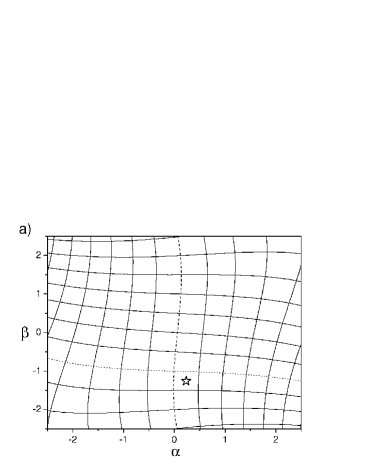
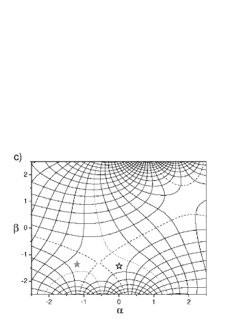
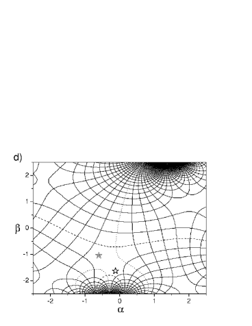
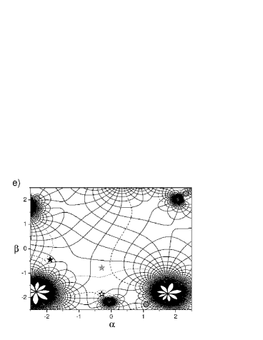
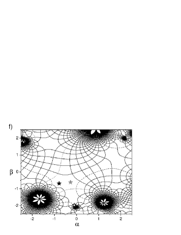
Figure 1: Curves of constant $Q^{\prime\prime}$ superimposed with those of constant $P^{\prime\prime}$ in the $w$ plane. Dashed lines refer to $Q^{\prime\prime}=0$ and the dotted lines to $P^{\prime\prime}=0$. From panel (a) to (f), the value of $T$ is to $T=0.06,\,0.24,\,0.70,\,1.02,\,2.20$ and $2.70$, respectively. Stars are centered at the point $Q^{\prime\prime}=P^{\prime\prime}=0.5$. White stars represent trajectories belonging to the family $f1$, grey stars to $f2$, and the black stars to $f3$. The circles in panel (e) also represent potential candidates to be included in the sum (16), illustrating the existence of other trajectories satisfying the proper boundary conditions (15). In this case, since they lie far from the origin, they were not included in the calculation.

         

            

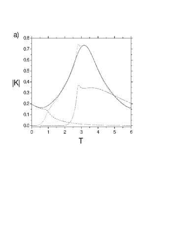
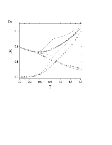
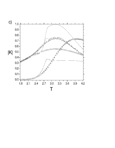
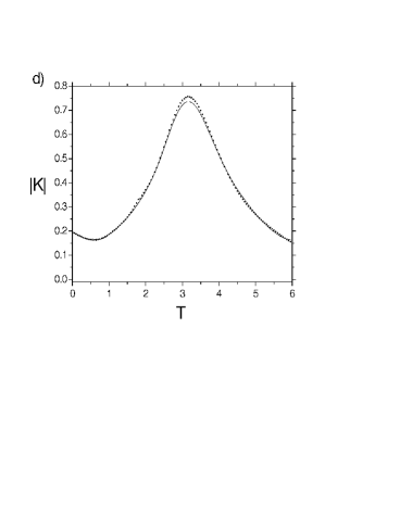
Figure 2: Exact propagator (full line in all panels) and semiclassical results for $K^{(2)}_{sc}(z^{\prime\prime*},z^{\prime},T)$ and $K^{un}_{sc}(z^{\prime\prime*},z^{\prime},T)$ for the quartic oscillator. Panel (a) shows the exact result and the individual contribution of each family of complex trajectories to $K^{(2)}_{sc}$: $f1$ (dashed), $f2$ (dotted) and $f3$ (dash-dotted). Panel (b) shows the propagator for $T<1.8$ and displays the exact result, the contributions of $f1$ (dashed) and $f2$ (dotted) and the combined contributions of $f1$ and $f2$ (dash-dotted). The uniform propagator $K^{un}_{sc}$ calculated with $f1$ and $f2$ is also shown, evaluated for each possible path: $C_{1}$ (squares), $C_{2}$ (circles) and $C_{3}$ (triangles). Panel (c) focuses on the interval $1.8<T<4.2$ and shows the exact result, the contributions of $f2$ (dotted) and $f3$ (dash-dotted) and the combined contributions of $f2$ and $f3$ (dashed). The uniform propagator calculated with $f2$ and $f3$ is also shown along the three independent paths. Panel (d) shows the final result obtained with the uniform formula (dots) and exact result.

In order to find complex trajectories satisfying the boundary conditions (15) we follow the recipe of Rubin and Klauder [13] and define

$$Q(0)=q^{\prime}+w\quad\mathrm{and}\quad P(0)=p^{\prime}+i\frac{b}{c}w,$$ (41)

where $w=\alpha+i\beta$ is a complex number. It is easy to check that this choice of initial conditions satisfy the first of the boundary conditions (15) for all values of $w$. The idea, therefore, is to propagate trajectories for all possible $w$, picking those satisfying the second of the boundary conditions (15). Specifically, for each $w$ we propagate the complex trajectory starting from (41) and calculate

$$v(T)\equiv v_{T}=\frac{1}{\sqrt{2}}\left(\frac{Q(T)}{b}-i\frac{P(T)}{c}\right)\equiv\frac{1}{\sqrt{2}}\left(\frac{Q^{\prime\prime}}{b}-i\frac{P^{\prime\prime}}{c}\right),$$ (42)

where $Q(T)$ and $P(T)$ are complex and $Q^{\prime\prime}$ and $P^{\prime\prime}$ are real variables, obtained by taking the real and imaginary parts of $v_{T}$. The trajectories for which $(Q^{\prime\prime},P^{\prime\prime})=(q^{\prime\prime},p^{\prime\prime})$ are the ones needed to calculate $K_{sc}^{(2)}(z^{\prime\prime*},z^{\prime},T)$ and $K_{sc}^{un}(z^{\prime\prime*},z^{\prime},T)$.

Notice that the origin $\alpha=\beta=0$ corresponds to the real trajectory starting from $Q(0)=q^{\prime}$, $P(0)=p^{\prime}$. Therefore, the larger the $|w|$ the more complex is the corresponding trajectory and the smaller its contribution to the propagator. Thus, we can restrict our search to a small vicinity of the origin in the complex $w$ plane.

By fixing $q^{\prime}$, $p^{\prime}$ and $T$, the values of the resulting $Q^{\prime\prime}$ and $P^{\prime\prime}$ can be seen as function of $w$. In Fig. 1 we represent the curves of constant $Q^{\prime\prime}$ superimposed with those of constant $P^{\prime\prime}$ for different values of $T$ in the $(\alpha,\beta)$ plane. Stars identify the points where $Q^{\prime\prime}=q^{\prime\prime}=0.5$ and $P^{\prime\prime}=p^{\prime\prime}=0.5$, our desired final values. As $T$ is changed, the position of the stars move in the $w$ plane, forming families of contributing trajectories. Circles (only in Fig. 1(e)) are the same as stars, but their contributions were not included because they lie very far from the origin.

White stars in Fig. 1 represent trajectories belonging to the family $f1$, which are close to the origin when $T=0$ but move away as $T$ increases. Grey stars refer to the family $f2$. Trajectories belonging to this family start off quite complex, but approach the origin of the $w$ plane as $T$ tends to $3.2$, approximately. After that, they move away from the origin again. Finally, trajectories of the family $f3$ are represented by black stars. They give important contributions for $T>2$. Other trajectories satisfying these same boundary conditions exist (see Fig. 1(e)) but their contribution to the propagator is not significant.

For $T=0$, a contour plot like those in Fig. 1 would display a grid of straight lines, vertical for $Q^{\prime\prime}=const.$ and horizontal for $P^{\prime\prime}=const.$, with the only contributing trajectory lying at $\alpha=1/4,~{}\beta=-5/4$. For short values of $T$, as in Fig. 1(a) for $T=0.06$, the grid deforms slightly and the contributing trajectory moves away from the origin. For $T=0.24$, Fig. 1(b), there is still a single contributing trajectory, but two defects on the grid are seen approaching the origin. As discussed in Refs. [13, 30], these defects are critical points of the map $v_{T}=v_{T}(w)$, where $\frac{\partial Q^{\prime\prime}}{\partial w}=\frac{\partial P^{\prime\prime}}{\partial w}=0$. In addition, if the second derivatives of $Q^{\prime\prime}$ and $P^{\prime\prime}$ are non-zero, it can be shown that the map becomes two-to-one in the vicinity of the defects, implying two different trajectories (corresponding to two distinct initial conditions) satisfying the same boundary conditions (15). These defects, therefore, can be identified with the phase space caustics.

For $T=0.70$ and $T=1.02$, panels (c) and (d), two complex trajectories can be seen and for $T=2.20$ and $T=2.70$, panels (e) and (f), three of them are close to the origin. For $T=2.70$, the trajectories belonging to $f2$ and $f3$ are the closest they get to each other, moving away for larger $T$. The effect of the nearby caustic should be pronounced at this point.

Figure 2(a) shows the exact propagator and the individual contribution of each family, $f1$, $f2$ and $f3$, to the propagator $K^{(2)}_{sc}(z^{\prime\prime*},z^{\prime},T)$ for $0\leq T\leq 6$. For very short times the contribution of $f1$ is clearly dominant, and reproduces very well the exact results by itself. For $T>0.5$ the family $f2$ becomes more and more important, whereas the contribution of $f1$ decreases. However, for $T\approx 1.0$ the exact curve is not reproduced by $f1$ nor by $f2$, suggesting that both families should be included simultaneously.

Figure 2(b) shows a detailed plot for the interval $0\leq T<1.8$ of such a combined contribution. The result obtained is clearly not accurate. However, by looking at Fig. 1, we notice that these trajectories are close to a phase space caustic, and, therefore, a divergent behavior is expected. Results for $K^{un}_{sc}(z^{\prime\prime*},z^{\prime},T)$ are presented in the same panel (b) for each possible integration path, $C_{1}$, $C_{2}$ and $C_{3}$ (see equation (39)). Choosing the path $C_{1}$ for $0\leq T<0.65$, and $C_{3}$ for $0.65\leq T<1.8$, the exact result is satisfactorily reproduced.

Returning to Fig. 2(a), we noticed that, after $T\approx 1.8$, the family $f2$ reproduces the exact result by itself, except for the vicinity of $T\approx 2.7$. As the family $f3$ gives relevant contributions in this interval, we plot the combined contributions of $f2$ and $f3$ in Fig. 2(c). The resulting curve is clearly inaccurate and the reason is, once again, the proximity of these trajectories to a caustic, as can be seen from Fig. 1(f). Thus, we use again the uniform formula $K^{un}_{sc}(z^{\prime\prime*},z^{\prime},T)$ (now for families $f2$ and $f3$), and the resulting curves are shown in Fig. 2(c). Path $C_{3}$ should be chosen for $1.8\leq T<2.55$, and $C_{1}$, for $T\geq 2.55$, so that the exact curve is well reproduced.

Fig. 2(d) shows the uniform approximation for the whole time interval $0<T<6$, obtained by joining four pieces of the propagator: (a) families $f1$ and $f2$ with path $C_{1}$ for $T<0.65$; (b) families $f1$ and $f2$ with path $C_{3}$ for $0.65\leq T<1.8$; (c) families $f2$ and $f3$ with path $C_{3}$ for $1.8\leq T<2.55$; (d) families $f2$ and $f3$ with path $C_{1}$ for $T\geq 2.55$.

We note that the trajectories of the $f3$ family do not seem to contribute to Eq. (16), since their inclusion makes the results worse everywhere. However, as they become partners of the contributing trajectories belonging to $f2$ (when these approach the caustic), their contributions become fundamental to control the divergence of the family $f2$ when Eq. (38) is used.

7 The Nelson potential

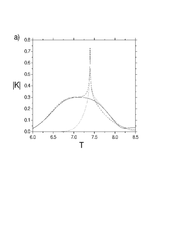
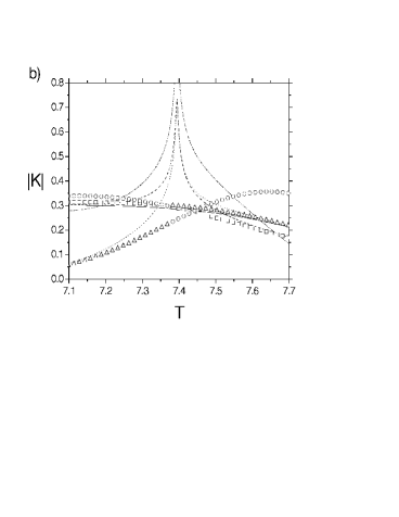
Figure 3: Comparison between the exact propagator and the two semiclassical approaches for the Nelson potential. Panel (a) shows the exact curve (full line) and the individual contribution of two families of complex trajectories (dashed lines for $f1$ and dotted lines for $f2$) to $K^{(2)}_{sc}$. Panel (b) shows a blow up in the caustic region. The dash-dotted line corresponds to the combined contribution of the two families of trajectories. The uniform propagator is also shown for the paths $C_{1}$ (squares), $C_{2}$ (circles) and $C_{3}$ (triangles). Panel (c) shows the exact (full line) and final semiclassical results (dashed line).

In the previous sections, both the theory and the numerical example were presented for one-dimensional systems only. Here we show an application for a two-dimensional chaotic system. The derivation of expressions equivalent to (16) and (38) for this case can be found in references [21, 24, 34]. The second order and uniform semiclassical formulas are given by

$$K_{sc}^{(2)}(\mathbf{z}^{\prime\prime*},\mathbf{z}^{\prime},T)=\sum_{\mathrm{traj.}}\sqrt{\frac{1}{\left|\det\mathbf{\mathrm{M}_{vv}}\right|}}\,\exp{\left\{\frac{i}{\hbar}\,(\mathcal{S}+\mathcal{G})-\frac{1}{2}\left(|\mathbf{z}^{\prime}|^{2}+|\mathbf{z}^{\prime\prime}|^{2}\right)\right\}}$$ (43)

and

$$K_{sc}^{un}(\mathbf{z}^{\prime\prime*},\mathbf{z}^{\prime},T)=i\sqrt{\pi}~{}e^{\mathcal{A}}\left\{\left(\frac{h_{2}-h_{1}}{\sqrt{\mathcal{B}}}\right)\mathrm{f^{\prime}_{i}}(\mathcal{B})+(h_{1}+h_{2})\mathrm{f_{i}}(\mathcal{B})\right\}$$ (44)

where $|\mathbf{z}\rangle\equiv|z_{x}\rangle\otimes|z_{y}\rangle$ is the direct product of two 1-D states,

$$\mathcal{S}({\mathbf{z}^{\prime\prime}}^{*},\mathbf{z}^{\prime},T) = \int_{0}^{T}\left[\frac{i\hbar}{2}\left(\dot{\mathbf{u}}~{}\mathbf{v}-\mathbf{u}~{}\dot{\mathbf{v}}\right)-\tilde{H}\right]dt-\frac{i\hbar}{2}\left[{\mathbf{u}(T)~{}{\mathbf{z}^{\prime\prime}}^{*}+\mathbf{z}^{\prime}~{}\mathbf{v}(0)}\right],$$ (45)

$$\mathcal{G}({\mathbf{z}^{\prime\prime}}^{*},\mathbf{z}^{\prime},T) = \frac{1}{2}\int_{0}^{T}\left[\frac{\partial^{2}\tilde{H}}{\partial u_{x}\;\partial v_{x}}+\frac{\partial^{2}\tilde{H}}{\partial u_{y}\;\partial v_{y}}\right]\,dt,$$ (46)

$$\left(\begin{array}[]{c}\delta\mathbf{u}^{\prime\prime}\\ \delta\mathbf{v}^{\prime\prime}\\ \end{array}\right)=\left(\begin{array}[]{cc}\mathbf{\mathrm{M}_{uu}}&\mathbf{\mathrm{M}_{uv}}\\ \mathbf{\mathrm{M}_{vu}}&\mathbf{\mathrm{M}_{vv}}\\ \end{array}\right)\left(\begin{array}[]{c}\delta\mathbf{u}^{\prime}\\ \delta\mathbf{v}^{\prime}\\ \end{array}\right)$$ (53)

and

$$h_{1,2}=\sqrt{\mp\frac{\sqrt{\mathcal{B}}}{\left.\left(\det\mathrm{M_{\mathbf{vv}}}\right)\right|_{\mathbf{u}^{\prime\prime}_{1,2}}}}~{}e^{\frac{i}{\hbar}{\left.\mathcal{G}\right|_{z_{1,2}}}}.$$ (54)

For the numerical application we have chosen the Nelson Hamiltonian,

$$H=\frac{1}{2}(p_{x}^{2}+p_{y}^{2})+{\left(y-x^{2}/2\right)}^{2}+0.05x^{2}.$$

This system has been widely studied both classically [35] and quantum mechanically [21]. In particular, the coherent state propagator and its semiclassical quadratic approximation were investigated in great detail in [21] and some strongly divergent semiclassical behavior due to the presence of phase space caustics were identified. Here we revisit this problem, using the same parameters for which the caustics were found and apply the uniform formula.

The widths of $|\mathbf{z}^{\prime}\rangle$ and $|\mathbf{z}^{\prime\prime}\rangle$ were fixed to $b_{x}=b_{y}=0.2$ and $\hbar=0.05$. The eight remaining parameters fixing the initial and final coherent states are: $x^{\prime}=x^{\prime\prime}=0.72$, $y^{\prime}=y^{\prime\prime}=0.24$, $p_{x}^{\prime}=p_{x}^{\prime\prime}=-0.75$ and $p_{y}^{\prime}=p_{y}^{\prime\prime}=-0.63$, which refer to a diagonal element of the propagator.

Two families of trajectories ($f1$ and $f2$) contribute to the propagator (43) when $T$ is varied from 6 to 8.5, as shown in Fig. 3(a). Family $f1$ reproduces very well the exact propagator for the range $6<T<7.2$, while $f2$ does the same for $7.6<T<8.5$. In the vicinity of $T\approx 7.4$, the semiclassical result shows a divergent behavior. As shown in Fig. 3(b), the combined contributions of these families only makes things worse. A careful analysis of the classical phase space shows that this region is close to a caustic [21]. Therefore, it is indicated to use expression (44) instead of (43). The results for the uniform approximation are shown in Fig. 3(b) for the paths $C_{1}$, $C_{2}$ and $C_{3}$. Taking path $C_{1}$ for $T<7.38$ and $C_{3}$ for $T\geq 7.38$ kills the divergence and the exact result is reproduced, as shown in Fig. 3(c).

8 Final Remarks

Focal points and caustics are well known sources of inaccuracies in semiclassical approximations. The most systematic way to derive semiclassical formulas that avoid such divergences is to use the method of Maslov, which consists basically of two steps. The first step is to compute the semiclassical propagator in a dual representation. The caustics in the original and the dual representations lie generically in different regions of phase space, so that at least one of the propagators is well behaved at any given point. The second step is to transform back to the representation of interest doing the corresponding integral by the stationary phase approximation, but expanding beyond the second order.

Coherent states lack a natural dual representation and we have defined one such representation in [23]. Although the transformation leading from the Bargmann to the dual form is not a simple Fourier transform like in the case of position and momentum, it leads to a similar Legendre transformation of the action in the semiclassical limit. With this representation in hand the second step of the Maslov method can be carried out as usual. It is not clear at this point if this alternative representation can be useful in other contexts and work in this direction is in progress.

Finally we remark that one of the few semiclassical approaches that naturally avoids caustics is the initial value representation of Herman and Kluk [36, 37, 38] (see also [39]), for which the tangent matrix elements, that go to zero at the caustic, appear in the numerator and do not lead to divergencies. However, convergence problems due to highly oscillatory contributions have been reported for chaotic systems [40], which also required the development of additional techniques and methods.

The authors acknowledge financial support from CNPq, FAPESP and FINEP. ADR especially acknowledges FAPESP for the fellowship $\#$ 04/04614-4. Wilhelm und Else Hereaus Foundation and Instituto do Milênio de Informação quântica – CNPq are gratefully acknowledged for providing financial support for the Blaubeuren meeting. We also acknowledge AFR de Toledo Piza, Marcel Novaes and Fernando Parisio for their important contributions.

9 References

References

- [1] Klauder J R and Skagerstan B S 1985 Coherent States. Applications in Physics and Mathematical Physics (Singapore: World Scientific)
- [2] Bargmann V 1961 Comm. on Pure and Appl. Math. 14 187
- [3] Glauber R 1963 Phys. Rev. 131 2766
- [4] Perelomov A 1986 Generalized Coherent States and their Applications (Berlin: Springer-Verlag)
- [5] Zhang W M, Feng D H and Gilmore R 1990 Rev. Mod. Phys. 62 , 867
- [6] Klauder J R 1978 Continuous Representations and Path Integrals, revisited Path Integrals (NATO Advanced Study Institute, Series B: Physics) ed G J Papadopoulos and J T Devreese (New York: Plenum)
- [7] Klauder J R 1979 Phys. Rev. D 19 2349
- [8] Weissman Y 1982 J. Chem. Phys. 76 4067
- [9] Solari H G 1986 J. Math. Phys. 27 1351
- [10] Kochetov E A 1998 J. Phys. A 31 4473
- [11] Baranger M, de Aguiar M A M, Keck F, Korsch H J and Schellaaß B 2001 J. Phys. A 34 7227
- [12] Adachi S 1989 Ann. Phys. (NY) 195 45
- [13] Rubin A and Klauder J R 1995 Ann. Phys. (NY) 241 212
- [14] Xavier A L Jr and de Aguiar M A M 1996 Ann. Phys. NY 252 458 \nonumXavier A L Jr and de Aguiar M A M 1996 Phys. Rev. A 54 1808 \nonumXavier A L Jr and de Aguiar M A M 1997 Phys. Rev. Lett. 79 3323
- [15] Grossmann F 1998 Phys. Rev. A 57 3256
- [16] Tanaka A 1998 Phys. Rev. Lett. 80 1414
- [17] Parisio F and de Aguiar M A M 2003 Phys. Rev. A 68 062112
- [18] Novaes M and de Aguiar M A M Phys. Rev. A 72 032105
- [19] Novaes M 2005 J. Math. Phys. 46 102102
- [20] van Voorhis T and Heller E J 2002 Phys. Rev. A 66 050501 \nonumvan Voorhis T and Heller E J 2003 J. Chem. Phys. 119 12153
- [21] Ribeiro A D, de Aguiar M A M and Baranger M 2004 Phys. Rev. E 69 066204
- [22] Shalashilin D V and Child M S 2004 Chem. Phys. 304 103
- [23] Ribeiro A D, Novaes M and Aguiar M A M de 2005 Phys. Rev. Lett. 95 050405
- [24] Ribeiro A D and de Aguiar M A M de 2007 Ann. Phys. (NY) (Preprint doi:10.1016/j.aop.2007.04.008)
- [25] Maslov V P and Feodoriuk M V 1981 Semi-Classical Approximations in Quantum Mechanics (Boston: Reidel)
- [26] Bleistein N and Handelsman R A 1986 Asymptotic Expansion of Integrals (New York: Dover Publications)
- [27] Stokes G G 1864 Trans. Camb. Phil. Soc. 10 106. Reprinted in 1966 Mathematical and physical papers. George Gabriel Stokes vol. IV (New York: Johnson)
- [28] Heading J 1962 An Introduction to Phase-Integral Methods (London: Methuen) \nonumFröman N and Fröman P O 1965 JWKB Approximation. Contributions to the Theory (Amsterdan: North-Holland) \nonumDingle R B 1973 Asymptotic Expansions: Their Derivation and Interpretation (London: Academic Press)
- [29] Shudo A and Ikeda K S 1995 Phys. Rev. Lett. 74 682 \nonumShudo A and Ikeda K S 1996 Phys. Rev. Lett. 76 4151
- [30] de Aguiar M A M, Baranger M, Jaubert L, Parisio F and Ribeiro A D 2005 J. Phys. A 38 4645
- [31] Parisio F and de Aguiar M A M 2005 J. Phys. A 38 9317
- [32] Berry M V and Mount K E 1972 Rep. Prog. Phys. 35 315
- [33] Chester C, Friedman B and Ursell F 1957 Proc. Camb. Phil. Soc. 53 599 \nonumBerry M V 1969 Sci. Prog. (Oxford) 57 43 \nonumBerry M V and Upstill C 1980 Catastrophe Optics: Morphologies of Caustics and Their Diffrection Patterns, Progress in Optics XVIII vol. 36, ed. E Wolf (Amsterdam: North-Holland) pp. 257-346 \nonumBerry M V 1989 Proc. R. Soc. London A 422 7 \nonumFricke S H, Balantekin A B and Uzer T 1991 J. Math. Phys. 32 3125
- [34] Braun C and Garg A 2007 J. Math. Phys. 48 32104
- [35] Baranger M, Davies K T R and Mahoney J H 1988 Ann. Phys. (NY) 186 95
- [36] Herman M F and Kluk E 1984 Chem. Phys. 91 27 \nonumKay K G 1994 J. Chem. Phys. 100 4377 \nonumKluk E, Herman M F and Davis H L 1986 J. Chem. Phys. 84 326
- [37] Miller W H 2002 Mol. Phys. 100 397
- [38] Kay K G 2006 Chem. Phys. 322 3
- [39] Zhang D H and Pollak E 2004 Phys. Rev. Lett. 93 140401
- [40] Wang H, Manolopoulos D and Miller W H 2001 J. Chem. Phys. 115 6317 \nonumPollak E and Liao L J 1998 J. Chem. Phys. 108 2733 \nonumBurant J C and Batista V S 2002 J. Chem. Phys. 116 2748