Simulating Black Hole White Dwarf Encounters

Abstract

The existence of supermassive black holes lurking in the centers of galaxies and of stellar binary systems containing a black hole with a few solar masses has been established beyond reasonable doubt. The idea that black holes of intermediate masses ($\sim 1000$ ${\rm M_{\odot}}$) may exist in globular star clusters has gained credence over recent years but no conclusive evidence has been established yet. An attractive feature of this hypothesis is the potential to not only disrupt solar-type stars but also compact white dwarf stars. In close encounters the white dwarfs can be sufficiently compressed to thermonuclearly explode. The detection of an underluminous thermonuclear explosion accompanied by a soft, transient X-ray signal would be compelling evidence for the presence of intermediate mass black holes in stellar clusters. In this paper we focus on the numerical techniques used to simulate the entire disruption process from the initial parabolic orbit, over the nuclear energy release during tidal compression, the subsequent ejection of freshly synthesized material and the formation process of an accretion disk around the black hole.

1. Introduction

The existence of two classes of black holes is well-established: supermassive black holes with masses beyond $10^{6}$ M_⊙ are thought to lurk in the centers of most galaxiesrichstone98 and black holes with just a few solar masses have been identified as the unseen components in X-ray binary systemslewin06 . Black holes with $M_{\rm bh}\sim 1000$ M_⊙, so-called “intermediate mass black holes”, represent a plausible, but so far still unconfirmed “missing link” between these two well-established classes of black holes. In recent years, the stellar dynamics in the centers of some globular clusters has been interpreted as being the result the gravitational interaction with an intermediate mass black holegebhardt02 ; gerssen02 ; gerssen03 ; gebhardt05 . Further circumstantial evidence comes from ultraluminous, compact X-ray sources in young star clusterszezas02 ; pooley06 and from n-body simulationsportegies04 that indicate that runaway collisions in dense young star clusters can lead to rapidly growing black holes. None of these arguments is conclusive by itself, but their different nature suggests that the possibility of intermediate mass black holes must be taken seriously.
The tidal disruption of white dwarfs offers the unique possibility to explore the presence of an intermediate mass black hole. The corresponding disruption processes have been explored with various approximations in earlier studies luminet89b ; wilson04 ; dearborn05 , our simulations for the first time explore the full evolution from the initial parabolic orbit over the disruption process to the subsequent build-up of an accretion disk. We have performed a large set of calculations to identify observational signatures that can corroborate or, alternatively, rule out the existence of intermediate mass black holes. In this paper we focus on the numerical techniques that have been employed in this disruption study, a detailed discussion of the astrophysical implications will be given elsewhererosswog07f ; rosswog07d .

2. Numerical methods

The simulation of a white dwarf disruption by a black hole needs to follow the gas dynamics from the initial spherical star through the distortion and compression while approaching the black hole to the subsequent expansion phase and the formation of an accretion disk. Of paramount importance for the dynamical evolution is the inclusion of the feedback from the nuclear reactions that are triggered by the tidal compression. In the following we will briefly sketch the methods employed in our simulations.

2.1. Hydrodynamics

Due to the highly variable geometry and the importance of the strict numerical conservation of physically conserved quantities, we use the smoothed particle hydrodynamics method (SPH) to discretize the equations of an ideal fluid. Using the SPH approximationsbenz90a ; monaghan05 the conservation of mass, momentum and energy translate into

$$\rho_{a} = \sum_{b}m_{b}W_{ab}$$ (1)

$$\frac{{d\vec{v}}_{a}}{dt} = -\sum_{b}m_{b}\left\{\frac{P_{a}}{\rho_{a}^{2}}+\frac{P_{b}}{\rho_{b}^{2}}+\Pi_{ab}\right\}\nabla_{a}W_{ab}+\vec{f}_{a,\rm grav}$$ (2)

$$\frac{du_{a}}{dt} = \frac{P_{a}}{\rho_{a}^{2}}\sum_{b}m_{b}\vec{v}_{ab}\nabla_{a}W_{ab}+\frac{1}{2}\sum_{b}m_{b}\Pi_{ab}\vec{v}_{ab}\nabla_{a}W_{ab}$$ (3)

$$+\dot{\epsilon}_{{\rm nuc},a}.$$

Here $\rho_{a}$ is the density at the position of particle $a$, $m_{b}$ the (constant) mass of particle $b$, $W_{ab}=W(|\vec{r}_{a}-\vec{r}_{b}|,h_{ab})$ the cubic spline kernelmonaghan85 with compact support whose width is set by the average of the smoothing lengths of particle $a$ and $b$, $h_{ab}=(h_{a}+h_{b})/2$. $P_{a}$ refers to the gas pressure, $\vec{f}_{a,\rm grav}$ to the gravitational acceleration of particle $a$ and $\Pi_{ab}$ is the artificial viscosity tensor, see below, and $\vec{v}_{ab}=\vec{v}_{a}-\vec{v}_{b}$ with $\vec{v}$ being the particle velocity. The quantity $u_{a}$ is the specific internal energy of particle $a$, $\dot{\epsilon}_{{\rm nuc},a}$ is the thermonuclear energy generation, calculated in a operator split fashion as described below. Since SPH is a Lagrangian method, and we ignore mixing, the compositional evolution is a local phenomenon.
In cases where the geometry of the gas distribution varies substantially, it is advisable to adapt the local resolution, i.e. the smoothing length, according to the changes in the matter density. We achieve this by scaling the smoothing length with the density according to

$$\frac{h_{a}(t)}{h_{a,0}}=\left(\frac{\rho_{a,0}}{\rho_{a}(t)}\right)^{1/3},$$ (4)

where the index $0$ labels the quantities at the beginning of the simulation. The initial smoothing lengths are chosen so that each particle has 100 neighbors. Taking the Lagrangian time derivative of both sides of Eq. (4) and using the Lagrangian form of the continuity equation, one finds an evolution equation for the smoothing length of each particle:

$$\frac{dh_{a}}{dt}=\frac{1}{3}h_{a}(\nabla\cdot\vec{v})_{a},$$ (5)

where

$$(\nabla\cdot\vec{v})_{a}=-\frac{1}{\rho_{a}}\sum_{b}m_{b}\vec{v}_{ab}\nabla_{a}W_{ab}.$$ (6)

This equation is integrated together with the other ODEs required for hydrodynamics, Eqs. (2), (3), (8), and possible changes in the abundances in the case of nuclear reactions. During the integration the resulting new neighbor number is constantly monitored for each particle and, if necessary, an iteration of the smoothing length is performed to keep the neighbor number in the desired range of between 80 and 120.
The SPH equations derived from a Lagrangianspringel02 ; monaghan02 yield different symmetries in the particle indices and additional multiplicative factors with values close to unity, but a recent comparisonrosswog07c between these two sets of equations showed only very minor differences in practical applications.
We use the artificial viscosity tensor in the form given in monaghan92 , but with the following important modifications: i) the viscosity parameters $\alpha$ and $\beta$ (commonly set to constants $\alpha=1$, $\beta=2$) are replaced by $\alpha\rightarrow\tilde{\alpha}_{ab}=(\alpha_{a}+\alpha_{b})(f_{a}+f_{b})/4$, $\beta\rightarrow 2\tilde{\alpha}_{ab}$, where $f_{k}$ is the so-called Balsara-switchbalsara95 to suppress spurious forces in pure shear flows, and ii) the viscosity parameter $\alpha_{k}$ is determined by evolving an additional equationmorris97 with a decay and a source termrosswog00 :

$$\frac{d\alpha_{a}}{dt}=-\frac{\alpha_{a}-\alpha_{\rm min}}{\tau_{a}}+S_{a}$$ (7)

with

$$S_{a}={\rm max}\left[-(\vec{\nabla}\cdot\vec{v})_{a}(\alpha_{\rm max}-\alpha_{a}),0\right].$$ (8)

In the absence of shocks $\alpha$ decays to $\alpha_{\rm min}$ on a time scale $\tau_{a}=h_{a}/(0.1\;c_{a})$, where $c_{a}$ is the sound velocity. In a shock $\alpha$ rises rapidly to capture the shock properly. A further discussion of this form of artificial viscosity can be found in rosswog02a .
To demonstrate the ability of this scheme to capture shocks without spurious post-shock oscillations we show in Fig. 1 the results of a standard, one-dimensional Sod shock tube testsod78 (with a polytropic gas of adiabatic exponent $\Gamma=1.4$) at t=0.17. For this test we used 1000 SPH particles, $\alpha_{\rm max}=1.5$ and $\alpha_{\rm min}=0.1$. The numerical solution (circles) agrees excellently with the exact solution (solid line), the shock itself is spread over about 10 particles. In the third panel (“pressure”) we have overlaid the value of the viscosity parameter $\alpha$. It deviates substantially from its minimum value only in the direct vicinity of the shock where it reaches values of about 1.3. This is to be compared to the “standard” values $\alpha=1$ and $\beta=2$ that are commonly applied in astrophysical simulations to each particle irrespective of the necessity to resolve a shock. This scheme has been shownrosswog00 ; rosswog02a to minimize possible artifacts due to artificial viscosity.
Note that no efforts have been made to include the effects of heat transport. Therefore, deflagration-type combustion cannot be handled adequately with the current code. As will be discussed below, deflagration is of no importance for the disruption processes that we discuss here.

2.2. Equation of state

The system of fluid equations (1), (2) and (3) needs to be closed by an equation of state (EOS) that is appropriate for white dwarf matter. We use the HELMHOLTZ EOS developed by the Center for Astrophysical Thermonuclear Flashes at the University of Chicago. It accepts an externally calculated nuclear composition which facilitates the coupling to reaction networks. The ions are treated as a Maxwell-Boltzmann gas, for the electron/positron gas the exact expressions are integrated numerically (i.e. no assumptions about the degree of degeneracy or relativity are made) and the result is stored in a table. A sophisticated, biquintic Hermite polynomial interpolation is used to enforce the thermodynamic consistency at interpolated valuestimmes00a . The photon contribution is treated as blackbody radiation. The EOS covers the density range form $10^{-10}\leq\rho Y_{e}\leq 10^{11}$ g cm^-3 ($Y_{e}$ being the electron fraction) and temperatures from $10^{4}$ to $10^{11}$ K.

2.3. Gravity

The self-gravity of the fluid is calculated via a parallel version of the binary tree described in benz90b . The same tree is used to search for the neighbor particles that are required for the density estimate, Eq. (1), and the gradients in Eqs. (2), (3) and (5). The gas acceleration due to a (Schwarzschild) black hole is treated in the Paczyński-Wiita approximationpac80 . This approach has been shownartemova96 to yield accurate results for the accretion onto non-rotating black holes. To avoid numerical problems due to the singularity at the Schwarzschild radius the pseudo potential is smoothly extended in a non-singular way down to the holerosswog05a with an absorbing boundary placed at a distance of $3GM_{\rm bh}/c^{2}$ from the black hole with mass $M_{\rm bh}$.

2.4. A minimal nuclear reaction network

To address whether tidal compression can trigger a thermonuclear explosion, we need to evolve the nuclear composition and to include the feedback onto the gas from the energy released by nuclear burning. Running a full nuclear network with hundreds of species for each SPH particle would be computationally prohibitive, therefore a “minimal” network designed to provide the accurate energy generationhix98 ; timmes00b is used. It couples a conventional $\alpha$-network stretching from He to Si with a quasi-equilibrium-reduced $\alpha$-network. The QSE-reduced network neglects reactions within small equilibrium groups that form at temperatures above 3.5 GK to reduce the number of abundance variables needed. Although a set of only seven nuclear species is used, this network reproduces all burning stages from He-burning to nuclear statistical equilibrium accurately. For more details and tests we refer to hix98 .
In the presence of nuclear reactions the energy produced (or consumed) by nuclear reactions is given by

$$\dot{\epsilon}_{\rm nuc,a}=N_{\rm A}\sum_{j}B_{j}\frac{dY_{j,a}}{dt},$$ (9)

where $N_{\rm A}$ is Avogadro’s number, $B_{j}$ is the nuclear binding energy of the nucleus $j$, $Y_{j,a}=n_{j,a}/(\rho_{a}N_{\rm A})$ its abundance and $n_{j,a}$ is the number density of species $j$. Again, the subscript $a$ indicates that these quantities are evaluated at the position of particle $a$.
Since the nuclear reaction and the hydrodynamic time scales can differ by many orders of magnitude, the network is coupled to the hydrodynamics in an operator splitting fashion. In a first step, Eqs. (2),(3),(5),(8) are integrated forward in time via a MacCormack predictor-corrector schemelomax01 with individual time stepsrosswog07c to obtain new quantities at time $t^{n+1}$. In this step we ignore the nuclear source term in Eq. (3), the result is denoted by $\tilde{u}_{a}^{n+1}$. This value has to be corrected for the energy release that occurred from $t^{n}$ to $t^{n+1}$:

$$\epsilon_{a,n\rightarrow n+1} = N_{\rm A}\sum_{j}B_{j}\int_{t^{n}}^{t^{n+1}}\frac{dY_{j,a}}{dt}(\rho_{a}(t),T_{a}(t),Y_{k,a}(t))dt$$ (10)

$$= N_{A}\sum_{j=1}B_{j}(Y_{j,a}^{n+1}-Y_{j,a}^{n}),$$ (11)

where $\rho_{a}(t)\approx\rho_{a}(t^{n})+\frac{t-t^{n}}{t^{n+1}-t^{n}}\{\rho_{a}(t^{n+1})-\rho_{a}(t^{n})\}$ and $T_{a}(t)\approx T_{a}(t^{n})$ has been used to integrate the abundances $Y_{j,a}$ via the implicit backward Euler method (the network integration is described in detail inhix98 ). The final value for the specific energy at time $t^{n+1}$ is given by

$$u_{a}^{n+1}=\tilde{u}_{a}^{n+1}+\epsilon_{a,n\rightarrow n+1}.$$ (12)

Now the EOS is called again to make all thermodynamic quantities consistent with this new value $u_{a}^{n+1}$. Once the derivatives have been updated, the procedure can be repeated for the next time step.
For the hydrodynamic time step we use the minimum of several criteria. We use a force criterion and a combination of Courant-type and viscosity-based criterionmonaghan92

$$\Delta t_{f,a}=\sqrt{h_{a}/|\vec{f}_{a}|}$$ (13)

and

$$\Delta t_{C,a}=\frac{h_{a}}{v_{{\rm s},a}+0.6(v_{{\rm s},a}+2\;{\rm max}_{b}\;\mu_{ab})},$$ (14)

where $\vec{f}_{a}$ is the acceleration, $v_{{\rm s},a}$ is the sound velocity and $\mu_{ab}$ a quantity used in the artificial viscosity tensor (for its explicit form see monaghan92 ). To ensure a close coupling between hydrodynamics and nuclear reactions in regions where burning is expected, we apply two additional time step criteria. One triggers on matter compression, the other on the distance to the black hole:

$$\Delta t_{\rm comp,a}=-0.03/(\nabla\cdot\vec{v})_{a}$$ (15)

and

$$\Delta t_{\rm bh,a}=0.03/\sqrt{GM_{\rm bh}/r_{\rm bh,a}^{3}}.$$ (16)

The “desired” hydro time step of each particle is then chosen as

$$\Delta t_{{\rm des},a}=0.2\;{\rm min}(\Delta t_{f,a},\Delta t_{C,a},\Delta t_{\rm comp,a},\Delta t_{\rm bh,a}).$$ (17)

How these desired time steps are transformed into the individual block time steps is explained in detail inrosswog07c . As a test, low-resolution versions of the production runs were run once with this time step prescription and once with halved time steps. No noticeable differences could be found.
One may wonder whether neutrino emission could subduct substantial amounts of energy during the burning phase. To test for this, we have plotted in Fig. 2 the ratio of the nuclear energy produced and the energy lost to neutrinos within a typical pericentre passage of 1 s duration. For the neutrino emission pair annihilation, plasma, photoneutrino, bremsstrahlung and recombination processes were considered according to the fit formulae of itoh96 as coded by F. Timmes. For the conditions relevant to this study neutrino emission was never relevant.

3. Results

As initial condition we set up a white dwarf on a parabolic orbit around the black hole with an initial separation of several tidal radii $R_{\rm tid}=R_{\rm WD}\left(\frac{M_{\rm bh}}{M_{\rm WD}}\right)^{1/3}$. In a large set of simulations we explored black hole masses of 100, 500, 1000, 5000 and 10 000 ${\rm M_{\odot}}\;$and white dwarf masses of 0.2, 0.6 and 1.2 ${\rm M_{\odot}}$. Each time several “penetration factors”, $P=R_{\rm tid}/R_{\rm peri}$, where $R_{\rm peri}$ is the pericentre separation, were explored. To be conservative, we set the initial white dwarfs to very low temperatures ($T_{0}=5\cdot 10^{4}$ K). The numerical resolution varied from 500 000 to more than $4\cdot 10^{6}$ SPH particles. In all cases we found explosions (nuclear energy release larger than the white dwarf gravitational binding energy) whenever the penetration factors exceeded values of about 3. Further details of these simulations will be discussed elsewhererosswog07d .
For conciseness we focus here on one exemplary simulation of a 0.2 ${\rm M_{\odot}}$, pure He white dwarf (modeled with more than $4\cdot 10^{6}$ SPH particles) and a 1000 ${\rm M_{\odot}}\;$black hole, see Fig. 3. The first snapshot (0.12 minutes after the simulation start) shows the stage of maximum white dwarf compression at pericentre passage, in which the white dwarf is also severely compressed perpendicular to the orbital plane. The peak compression occurs at a spatially fixed point (seen as the density peak in Fig. 3, left). The white dwarf fuel is fed with free-fall velocity $v_{\rm ff}=(2GM_{\rm bh}/R_{\rm peri})^{1/2}=1.6\cdot 10^{5}{\rm km\;s}^{-1}\;\left(M_{\rm bh}/1000{\rm M}_{\odot}\right)^{1/2}\left(R_{\rm peri}/10^{4}{\rm km}\right)^{-1/2}$ into this compression point. The comparison with typical flame propagation speeds ($\sim 100$ km/s) shows that combustion effects can be safely neglected for this investigation.
During the short compression time (of order one second), the peak density increases by more than one order of magnitude (with respect to the initial, unperturbed star) to $>6\cdot 10^{5}$ g cm^-3, the peak temperatures get close to nuclear statistical equilibrium ($>3.9\cdot 10^{9}$ K). During this stage 0.11 ${\rm M_{\odot}}\;$are burnt, mainly into silicon group (74%), iron group (22.5%) elements and carbon. The nuclear energy release triggers a thermonuclear explosion of the white dwarf. Since a much smaller fraction ends up in iron group nuclei (nickel), this explosion is underluminous in comparison to a normal type I a supernova which produces $\sim 0.5$ ${\rm M_{\odot}}\;$of nickel. Due to the very different geometry, the lightcurves of such explosions are expected to deviate substantially from standard type Ia light curves. This topic deserves further detailed investigations.
About 35 % of the initial stellar mass remain gravitationally bound to the black hole and will subsequently by accreted. During infall, matter trajectories become radially focused towards the pericentre. The large spread in the specific energy across the accretion stream width produces a large spread of apocentric distances and thus a fan-like spraying of the white dwarf debris after pericentre passage. This material interacts with the infalling material in an angular momentum redistribution shock, see Fig. 4, which results in the circularization of the forming accretion disk. The subsequent accretion onto the black hole produces a soft X-ray flare close the Eddington-luminosity for a duration of months.
For other combinations of black hole and white dwarf masses with $P>3$ we found a similar behavior. Therefore, an underlumious thermonuclear explosion accompanied by soft X-ray flare may whistle-blow the existence of intermediate mass black holes in globular clusters. The rate of this particular type of explosion amounts to a few tenths of a percent of “standard” type Ia supernovae. Future supernova surveys such as SNF could be able to detect several of these events.

Acknowledgments
We thank Holger Baumgardt, Peter Goldreich, Jim Gunn, Piet Hut, Dan Kasen and Martin Rees for very useful discussions. The simulations presented in this paper were performed on the JUMP computer of the Höchstleistungsrechenzentrum Jülich. E. R. acknowledges support from the DOE Program for Scientific Discovery through Advanced Computing (SciDAC; DE-FC02-01ER41176). W. R. H. has been partly supported by the National Science Foundation under contracts PHY-0244783 and AST-0653376. Oak Ridge National Laboratory is managed by UT-Battelle, LLC, for the U.S. Department of Energy under contract DE-AC05-00OR22725.

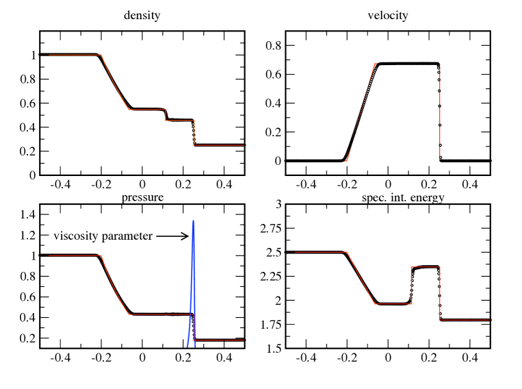
Figure 1.— Sod shock tube problem in 1D: the exact solution is given by the solid line, the numerical result is shown by the circles. In the lower left panel (pressure) the value of the time dependent artificial viscosity parameter $\alpha$ is overlaid. It is to be compared with the commonly used value $\alpha=1={\rm const}$.

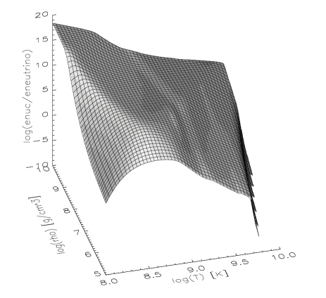
Figure 2.— Comparison of nuclear energy produced (from an initial pure He composition) and the energy lost via various neutrino reactions during 1 s (the typical pericentre passage time, see Fig. 3). The thick solid line that starts at about $\log(T)=9.1$ and ends at about $\log(T)=8.3$ shows the trajectory of the hottest 10% of the particles of the simulation shown in Fig. 3). To see clearly where neutrino emission becomes dominant, we have also thickened the contour where nuclear and neutrino contributions are equal.

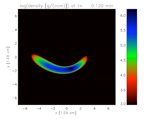
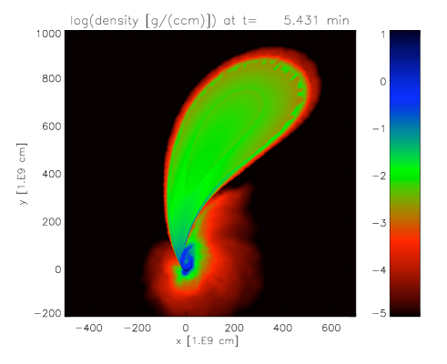
Figure 3.— Tidal disruption of a 0.2 M_⊙ He white dwarf by a 1000 M_⊙ black hole (located at the origin).

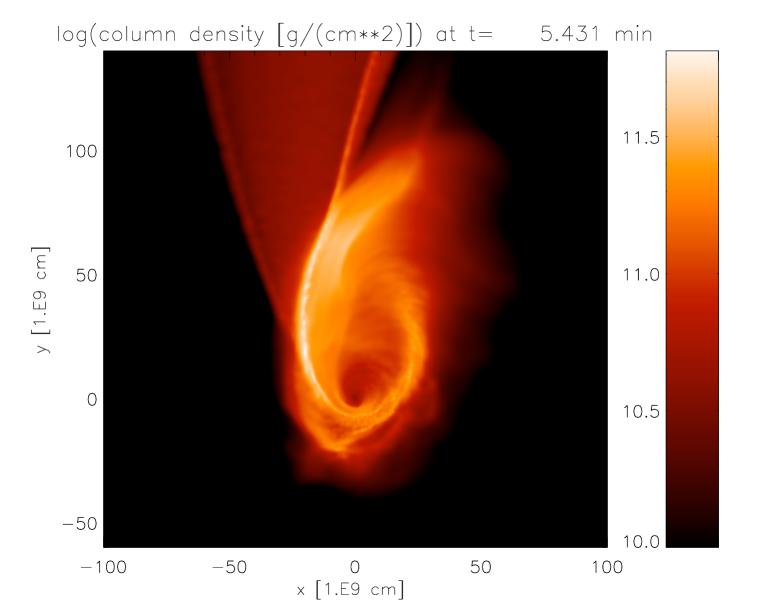
Figure 4.— Zoom-in on the forming accretion disk. Color-coded is the column density (in g/cm²), angular momentum is redistributed in the shock that forms when the accretion stream interacts with itself.

References

- (1) I. V. Artemova, G. Bjoernsson, I. D. Novikov, Modified Newtonian Potentials for the Description of Relativistic Effects in Accretion Disks around Black Holes, ApJ 461 (1996) 565.
- (2) D. Balsara, von neumann stability analysis of smooth particle hydrodynamics–suggestions for optimal algorithms, J. Comput. Phys. 121 (1995) 357.
- (3) W. Benz, Smooth particle hydrodynamics: A review, in: J. Buchler (ed.), Numerical Modeling of Stellar Pulsations, Kluwer Academic Publishers, Dordrecht, 1990, p. 269.
- (4) W. Benz, R. Bowers, A. Cameron, W. Press, ApJ 348 (1990) 647.
- (5) D. S. P. Dearborn, J. R. Wilson, G. J. Mathews, Relativistically Compressed Exploding White Dwarf Model for Sagittarius A East, ApJ 630 (2005) 309–320.
- (6) K. Gebhardt, R. M. Rich, L. C. Ho, A 20,000 M⊙ Black Hole in the Stellar Cluster G1, ApJL 578 (2002) L41–L45.
- (7) K. Gebhardt, R. M. Rich, L. C. Ho, An Intermediate-Mass Black Hole in the Globular Cluster G1: Improved Significance from New Keck and Hubble Space Telescope Observations, ApJ 634 (2005) 1093–1102.
- (8) J. Gerssen, R. P. van der Marel, K. Gebhardt, P. Guhathakurta, R. C. Peterson, C. Pryor, Hubble Space Telescope Evidence for an Intermediate-Mass Black Hole in the Globular Cluster M15. II. Kinematic Analysis and Dynamical Modeling, AJ 124 (2002) 3270–3288.
- (9) J. Gerssen, R. P. van der Marel, K. Gebhardt, P. Guhathakurta, R. C. Peterson, C. Pryor, Addendum: Hubble Space Telescope Evidence for an Intermediate-Mass Black Hole in the Globular Cluster M15. II. Kinematic Analysis and Dynamical Modeling, AJ 125 (2003) 376–377.
- (10) W. R. Hix, A. M. Khokhlov, J. C. Wheeler, F.-K. Thielemann, The Quasi-Equilibrium-reduced alpha -Network, ApJ 503 (1998) 332–+.
- (11) N. Itoh, H. Hayashi, A. Nishikawa, Y. Kohyama, ApJ 339 (1989) 354.
- (12) W. H. G. Lewin, M. van der Klis, Compact stellar X-ray sources, Compact stellar X-ray sources, 2006.
- (13) H. Lomax, T. Pulliam, D. Zingg, Fundamentals of Computational Fluid Dynamics, Springer, Berlin, 2001.
- (14) J.-P. Luminet, B. Pichon, Tidal pinching of white dwarfs, A&A 209 (1989) 103–110.
- (15) J. Monaghan, J. Lattanzio, A refined particle method for astrophysical problems, A&A 149 (1985) 135.
- (16) J. J. Monaghan, Ann. Rev. Astron. Astrophys. 30 (1992) 543.
- (17) J. J. Monaghan, SPH compressible turbulence, MNRAS 335 (2002) 843–852.
- (18) J. J. Monaghan, Smoothed particle hydrodynamics, Reports of Progress in Physics 68 (2005) 1703–1759.
- (19) J. Morris, J. Monaghan, A switch to reduce sph viscosity, J. Comp. Phys. 136 (1997) 41.
- (20) B. Paczynsky, P. J. Wiita, Thick accretion disks and supercritical luminosities, A&A 88 (1980) 23–31.
- (21) D. Pooley, S. Rappaport, X-Rays from the Globular Cluster G1: Intermediate-Mass Black Hole or Low-Mass X-Ray Binary?, ApJL 644 (2006) L45–L48.
- (22) S. F. Portegies Zwart, H. Baumgardt, P. Hut, J. Makino, S. L. W. McMillan, Formation of massive black holes through runaway collisions in dense young star clusters, Nature 428 (2004) 724–726.
- (23) D. Richstone, E. A. Ajhar, R. Bender, G. Bower, A. Dressler, S. M. Faber, A. V. Filippenko, K. Gebhardt, R. Green, L. C. Ho, J. Kormendy, T. R. Lauer, J. Magorrian, S. Tremaine, Supermassive black holes and the evolution of galaxies., Nature 395 (1998) A14+.
- (24) S. Rosswog, Mergers of Neutron Star-Black Hole Binaries with Small Mass Ratios: Nucleosynthesis, Gamma-Ray Bursts, and Electromagnetic Transients, ApJ 634 (2005) 1202–1213.
- (25) S. Rosswog, M. B. Davies, High-resolution calculations of merging neutron stars - I. Model description and hydrodynamic evolution, MNRAS 334 (2002) 481–497.
- (26) S. Rosswog, M. B. Davies, F.-K. Thielemann, T. Piran, Merging neutron stars: asymmetric systems, A&A 360 (2000) 171–184.
- (27) S. Rosswog, E.Ramirez-Ruiz, R. Hix, Atypical thermonuclear supernovae from tidally crushed white dwarfs, ApJ, accepted, arXiv:0712.2513.
- (28) S. Rosswog, E.Ramirez-Ruiz, R. Hix, to be submitted.
- (29) S. Rosswog, D. Price, Magma: a magnetohydrodynamics code for merger applications, MNRAS 379 (2007) 915 – 931.
- (30) G. Sod, A survey of several finite difference methods for systems of nonlinear hyperbolic conservation laws, J. Comput. Phys. 43 (1978) 1–31.
- (31) V. Springel, L. Hernquist, Cosmological smoothed particle hydrodynamics simulations: the entropy equation, MNRAS 333 (2002) 649–664.
- (32) F. X. Timmes, R. D. Hoffman, S. E. Woosley, An Inexpensive Nuclear Energy Generation Network for Stellar Hydrodynamics, ApJS 129 (2000) 377–398.
- (33) F. X. Timmes, F. D. Swesty, The Accuracy, Consistency, and Speed of an Electron-Positron Equation of State Based on Table Interpolation of the Helmholtz Free Energy, ApJS 126 (2000) 501–516.
- (34) J. R. Wilson, G. J. Mathews, White Dwarfs near Black Holes: A New Paradigm for Type I Supernovae, ApJ 610 (2004) 368–377.
- (35) A. Zezas, G. Fabbiano, A. H. Rots, S. S. Murray, Chandra Observations of “The Antennae” Galaxies (NGC 4038/4039). III. X-Ray Properties and Multiwavelength Associations of the X-Ray Source Population, ApJ 577 (2002) 710–725.