Semifluxons in Superconductivity and Cold Atomic Gases

Abstract

Josephson junctions and junction arrays are well studied devices in superconductivity. With external magnetic fields one can modulate the phase in a long junction and create traveling, solitonic waves of magnetic flux, called fluxons. Today, it is also possible to device two different types of junctions: depending on the sign of the critical current density $j_{c}\gtrless 0$, they are called $0$- or $\pi$-junction. In turn, a $0$-$\pi$ junction is formed by joining two of such junctions. As a result, one obtains a pinned Josephson vortex of fractional magnetic flux, at the $0$-$\pi$ boundary. Here, we analyze this arrangement of superconducting junctions in the context of an atomic bosonic quantum gas, where two-state atoms in a double well trap are coupled in an analogous fashion. There, an all-optical $0$-$\pi$ Josephson junction is created by the phase of a complex valued Rabi-frequency and we a derive a discrete four-mode model for this situation, which qualitatively resembles a semifluxon.

Keywords: Long Josephson junction, sine-Gordon equation, fractional Josephson vortex, quantum tunneling, cold atoms, Bose-Einstein condensates

1 Introduction

During the past two decades, the field of cold atomic gases has come a long way starting from almost lossless trapping and cooling techniques [1] to reaching quantum degeneracy of Bosons and Fermions [2]. Many phenomena that are the hallmarks of condensed matter physics, whether in superfluid or superconducting materials [3], are revisited within this novel context. Due to the remarkable ease with which it is possible to isolate the key mechanisms from rogue processes, one can clearly identify phase transitions, for example, Bose-Einstein condensation, the Mott phase transition or the BEC-BCS crossover. Today however, degenerate gases are still at a disadvantage if we consider robustness, portability or the ability for a mass production compared to solid-state devices, which is the great achievement of the semiconductor industry. Strong attempts to miniaturize cold gas experiments [4, 5] and to make them portable [6, 7, 8, 9] are currently under way in many laboratories.

Due to the great importance and practical relevance of the Josephson effect in superconducting systems [10, 11, 12], it has also received immediate attention after the first realization of Bose-Einstein condensates [13, 14, 15, 16, 17, 18, 19, 20, 21, 22, 23, 24, 25]. In particular, the combination of optical lattices with ultracold gases [26, 27] has boosted the possibilities to investigate junction arrays experimentally. Remarkably, even the absence of phase-coherence between neighboring sites can lead to interference as demonstrated in [28]. The possibility to study atomic Josephson vortices in the mean field description was raised first in connection with the sine-Gordon equation [29, 30].

In the present article we will report on such a transfer of concepts from a superconducting device [31], i.e., in various realizations of Josephson junction arrays and their unusual state properties of traveling (fluxons) and pinned (semifluxons) magnetic flux quanta to an analogous set up for neutral bosonic atoms in a trap. In particular, we will investigate an all-optical $0$-$\pi$ Josephson junction that can be created with a jumping phase of an optical laser.

This article organized as follows: in Sec. 2, we will give a brief review of the current status of the superconductor physics of Josephson junctions. In particular, we will refer to the most relevant publications in this thriving field of fluxon and semifluxon physics; in Sec. 3, we will discuss a similar setup, which allows to find a pinned semifluxon in an atomic $0$-$\pi$ Josephson junction and we compare the results. Finally, we will discuss further open questions in a Conclusion.

2 Fluxons and Semifluxons in Superconductivity

The Josephson effect is a well established phenomenon in the solid state physics. A Josephson junction (JJ) consists of two weakly coupled superconducting condensates. JJs are usually fabricated artificially using low- or high-$T_{c}$ superconducting electrodes separated by a thin insulating (tunnel), normal metal, or some other (exotic) barrier. JJs can also be present intrinsically in a anisotropic layered high-$T_{c}$ superconductors such as Bi₂Sr₂Ca₁Cu₂O₈[32, 33].

The dc Josephson effect (flow of current through a Josephson junction without producing voltage drop, i.e. without dissipation) is expressed using the first Josephson relation, which in the simplest case has the form

$$I_{s}=I_{c}\sin(\phi),$$ (1)

where $I_{s}$ is the supercurrent flowing through the junction, $I_{c}$ is the critical current, i.e. the maximum supercurrent which can pass through the JJ, and $\phi=\theta_{2}-\theta_{1}$ is the difference between the phases of the quantum mechanical macroscopic wave functions $\psi_{1,2}=\sqrt{n_{s}}e^{i\theta_{1,2}}$ of the superconducting condensates in the electrodes.

Recent advances in physics and technology allow to fabricate and study the so-called $\pi$-Josephson junctions — junctions which formally have negative critical current $I_{c}<0$. This can be achieved by using a ferromagnetic barrier, i.e. in Superconductor-Ferromagnet-Superconductor (SFS) [34, 35, 36, 37, 38] or Superconductor-Insulator-Ferromagnet-Superconductor (SIFS) [39, 40] structures. One can also achieve the same effect using a barrier which effectively flips the spin of a tunneling electron, e.g. when the barrier is made of a ferromagnetic insulator [41], of a carbon nanotube [42] or of a quantum dot created by gating a semiconducting nanowire [43].

The change in the sign of a critical current has far going consequences. For example, analyze the Josephson energy (potential energy related to the supercurrent flow). In a conventional JJ with $I_{c}>0$

$$U(\phi)=E_{J}(1-\cos\phi)$$ (2)

and has a minimum at $\phi=0+2\pi n$ (the ground state), where $E_{J}=\Phi_{0}I_{c}/2\pi$ is the Josephson energy. If $I_{c}<0$, we define $E_{J}=\Phi_{0}|I_{c}|/2\pi>0$ and

$$U(\phi)=E_{J}(1+\cos\phi).$$ (3)

Obviously, the minimum of energy is reached for $\phi=\pi+2\pi n$. Thus, in the ground state (the JJ is not connected to a current source, no current flows through it) the phase drop across a conventional JJ with $I_{c}>0$ is $\phi=0+2\pi n$, while for a junction with $I_{c}<0$ it is $\phi=\pi+2\pi n$. Therefore, one speaks about “$0$-JJs” and “$\pi$-JJs”.

Further, connecting the two superconducting electrodes of a $\pi$-JJ by a not very small inductor $L$ (superconducting wire), the supercurrent $\propto\pi/L$ will start circulating in the loop. Note, that this supercurrent is spontaneous, i.e., it appears by itself, and has a direction randomly chosen between clockwise and counterclockwise [44]. The magnetic flux created by this supercurrent inside the loop is equal to $\Phi_{0}/2$, where $\Phi_{0}=h/2e\approx 2.07\cdot 10^{-15}$ Wb is the magnetic flux quantum. Thus, the $\pi$-JJ works as a phase battery. This phase battery will work as described, supplying a supercurrent through the loop with inductor, provided the inductance $L\gg\Phi_{0}/I_{c}$. If the inductance $L$ is not that large, the battery will be over loaded, providing a smaller phase drop and supporting smaller current. For very small inductance the battery will stop working completely.

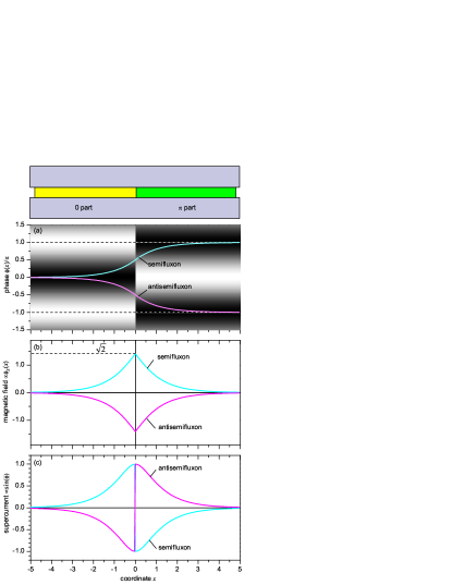
Figure 1: Sketch of a $0$-$\pi$ JJ and profiles of (a) the phase $\phi(x)$, (b) the magnetic field $\propto d\phi(x)/dx$ and (c) the supercurrent density $j_{s}(x)\propto\sin\phi(x)$ corresponding to a semifluxon (black) and antisemifluxon (gray).

Similar effects can be observed in a $\pi$ dc superconducting quantum interference device (SQUID: one $0$-JJ, one $\pi$-JJ and an inductor $L$ connected in series and closed in a loop) or in $0$-$\pi$ Josephson junction. Let us focus on a latter case.

Consider a long (along $x$) Josephson junction (LJJ) one half of which at $x<0$ has the properties of a $0$-JJ (critical current density $j_{c}>0$) and another half at $x>0$ has the properties of a $\pi$-JJ (critical current density $j_{c}<0$). Long means that the length is much larger than the so called Josephson length $\lambda_{J}$, which characterizes the size of a Josephson vortex; typically $\lambda_{J}\sim 10-20\,\mu$m. What will be the ground state of such a 0-$\pi$ LJJ? It turns out that if the junction is long enough (formally infinitely long), then far away from the $0$-$\pi$ boundary situated at $x=0$, i.e., at $x\to\pm\infty$ the phase $\phi$ will have the values 0 or $\pm\pi$ (we omit $2\pi n$ here), while in the vicinity of $0$-$\pi$ boundary the phase $\phi(x)$ smoothly changes from $\phi(-\infty)=0$ to $\phi(+\infty)=\pm\pi$, see Fig. 1a. The exact profile can be derived analytically [45, 46, 31]. Since the phase bends, the local magnetic magnetic field $H\propto d\phi/dx$ will be localized in the vicinity of the 0-$\pi$ boundary and carry the total flux equal to $\pm\Phi_{0}/2$, see Fig. 1b. The sign depends on whether the phase bends from $\phi(-\infty)=0$ to $\phi(+\infty)=+\pi$ or to $\phi(+\infty)=-\pi$. Thus, such an object is called a semifluxon or an antisemifluxon. If one analyzes the Josephson supercurrent density flowing though the barrier $j_{s}(x)=j_{c}(x)\sin\phi(x)$, one can see in Fig. 1c that the supercurrent has different directions on different sides from the $0$-$\pi$ boundary. Since we do not apply any external current, the flow of current should close in the top and bottom electrodes, i.e. the supercurrent circulates (counter)clockwise in the case of (anti)semifluxon. Thus, a semifluxon is a Josephson vortex of supercurrent. It is pinned at the $0$-$\pi$ boundary and has two degenerate ground states with the localized magnetic field carrying the flux $\pm\Phi_{0}/2$.

Semifluxons in various types of JJ has been actively investigated during the last years. In fact, the first experiments became possible because of deeper understanding the symmetry of the superconducting order parameter in cuprate superconductors. This order parameter with the so-called $d$-wave symmetry is realized in anisotropic superconductors, such as YBa₂Cu₃O₇ or Nd_2-xCe_xCuO₄. It allowed to fabricate $0$-$\pi$ grain boundary LJJs [47, 48] and, later, more controllable d-wave/s-wave ramp zigzag JJs [49, 50] and directly see and manipulate semifluxons using a SQUID microscope [51, 52].

Semifluxons are very interesting non-linear objects: they can form a variety of ground states [53, 54, 55, 56], may flip [51, 47] emitting a fluxon [57, 55, 58], or be rearranged [59] by a bias current. Huge arrays of semifluxons were realized [51] and predicted to behave as tunable photonic crystals [60]. Semifluxons are also promising candidates for storage devices in the classical or quantum domain and can be used to build qubits [61] as they behave like macroscopic spin $1/2$ particles.

Now, an interesting question arises: Can one realize $\pi$ or even 0-$\pi$ JJs in an atomic BEC? In the latter case, the degenerate ground state corresponding to a semifluxon should have a non-trivial spatial phase profile and semifluxon physics can also be studied using BEC implementation.

3 Semifluxons in Bose-Einstein Condensates

Here, we will address this question and examine a configuration were the two-state atoms are trapped in a quasi-one dimensional cigar-shaped trap with an additional superimposed double well potential in the longitudinal direction. The spatial localization of the two-state atoms inside the double well potential leads to two internal atomic Josephson junctions that are driven via an optical, complex valued “$0$-$\pi$” laser field and they are motionally connected via tunneling.

First, we will describe details of the model and introduce the Hamiltonian of the system. Then, we will examine the classical limit of the field theory and study the ground state of the Gross-Pitaevskii equation. Finally, we will exploit the fact that the spatial wavefunctions are localized inside a deep double well and study a simple four-mode quantum model derived from a Wannier basis state representation.

3.1 $0$-$\pi$-junction in a Bose-Einstein condensate

To model the $0$-$\pi$-Junction [29, 30] in a BEC, we are guided by the the condensed matter physics setup depicted in Fig. 2. As in the single atom case, we replace the two superconductors by an atomic two-level BEC in a cigar shaped trap. The two states of the atom, i.e., the excited state $|{e}\rangle$ and ground state $|{g}\rangle$ couple via a position dependent Rabi frequency $\Omega_{0}(x)$, which exhibits a phase jump at the origin of the $x$-axes

$$\Omega_{0}(x)=\left\{\begin{array}[]{ll}\Omega_{0},&x<0,\\ \Omega_{1}=-\Omega_{0},&x\geq 0.\end{array}\right.$$ (4)

Figure 2: Analogy of a $0$-$\pi$ Josephson junction in a superconductor (a) with an atomic two-level BEC (b) in a double well trap $V(x)$ with a position dependent Rabi frequency $\Omega_{0}(x)$. The excited atomic level $|{e}\rangle$ is separated from the ground level $|{g}\rangle$ by the detuning $2\delta$.

In this quasi one-dimensional scenario, we will represent the two-state atoms by a spinorial bosonic quantum field $\hat{\Psi}$, which satisfies the commutator relation

$$[\hat{\Psi}(x),\hat{\Psi}(y)^{\dagger}]=\mathds{1}\delta(x-y).$$ (5)

This field can be decomposed in any complete single particle basis $|{\sigma,l}\rangle$, which resolves the spatial extent of the field and the internal structure of the atoms, i.e.,

$$\hat{\Psi}=\sum_{\sigma=\{e,g\}}\sum_{l=0}^{\infty}|{\sigma,l}\rangle\,\hat{a}_{\sigma,l}$$ (6)

and we denote the corresponding discrete bosonic field amplitudes by $\hat{a}_{\sigma,l}$. Here, $\sigma$ characterizes the internal states by $(e,g)$ and the external motion in the double well potential by a quantum label $l$. The dynamical evolution of the atomic field is governed by following Hamiltonian

$$\hat{H} = \int_{-\infty}^{\infty}{\rm d}x\,\hat{\Psi}^{\dagger}(x)\left[-\partial^{2}_{x}+V(x)+\left(\begin{array}[]{cc}\delta&\Omega_{0}(x)\\ \Omega_{0}^{\ast}(x)&-\delta\end{array}\right)\right]\hat{\Psi}(x)$$

$$+g\hat{\Psi}_{e}^{\dagger}(x)\hat{\Psi}_{e}^{\dagger}(x)\hat{\Psi}_{e}^{\phantom{\dagger}}(x)\hat{\Psi}_{e}^{\phantom{\dagger}}(x)+g\hat{\Psi}_{g}^{\dagger}(x)\hat{\Psi}_{g}^{\dagger}(x)\hat{\Psi}_{g}^{\phantom{\dagger}}(x)\hat{\Psi}_{g}^{\phantom{\dagger}}(x).$$

In here, we use dimensionless units, in particular we have set $\hbar=1$ and the mass of the atom $m=1$. The energy consists of the single particle energy in a trap $V(x)$, which is identical for both species, the electric dipole interaction of the two-state atom [62], as well as a generic collision energy proportional to the coupling constant $g=g_{ee}=g_{gg}$. To simplify the analysis, we have deliberately set the cross-component scattering length $g_{eg}=0$. No unaccounted loss channels are present. Therefore, we have number conservation

$$\left[\hat{H},\hat{N}\right]=0,$$ (10)

as a symmetry. If we denote a generic state of the many-particle system in Fock-space by

$$|{\psi(t)}\rangle=\sum_{\mathbf{n}=0}^{\infty}\psi_{\mathbf{n}}(t)|{\mathbf{n}=(n_{0},n_{1},\ldots)}\rangle,$$ (11)

then one can obtain the dynamics of the system most generally from the Lagrangian formulation

$$\mathcal{L}[\psi_{\mathbf{n}}(t),\dot{\psi}_{\mathbf{n}}(t)]=\langle{\psi(t)}|i\partial_{t}-\hat{H}|{\psi(t)}\rangle.$$ (12)

In this field theory, the canonical momentum is given by $\pi_{\mathbf{n}}=\frac{\delta\mathcal{L}}{\delta\dot{\psi}_{\mathbf{n}}}=i\psi^{\ast}_{\mathbf{n}}$. From the Hamilton equation $\dot{\pi}_{\mathbf{n}}=-\frac{\delta\mathcal{L}}{\delta\psi_{\mathbf{n}}}$, one recovers the conventional Schrödinger equation in Fock space

$$i\partial_{t}|{\psi}\rangle=\hat{H}|{\psi}\rangle.$$ (13)

The Lagrangian approach is obviously a central concept in the path integral formulation of quantum mechanics [63]. However, it is also of great utility in the approximate description of the dynamics if we connect it with concepts of classical mechanics as we will see in the following.

3.2 Spatially extended classical model: the Gross-Pitaevskii equation

The classical limit of the field equations [2] can be recovered quickly by approximating the state of the system by a coherent state

$$\hat{\Psi}_{\sigma}(x)|{\psi}\rangle=\psi_{\sigma}(x)|{\psi}\rangle.$$ (14)

Within this approximation, we obtain from the Lagrangian of Eq. (12) the two component Gross-Pitaevskii equation $\psi=(\psi_{e}(x,t),\psi_{g}(x,t))^{\top}$

$$i\partial_{t}\psi=\left[-\partial^{2}_{x}+V(x)+\left(\begin{array}[]{cc}\delta+2g|\psi_{e}|^{2}&\Omega_{0}(x)\\ \Omega^{\ast}_{0}(x)&-\delta+2g|\psi_{g}|^{2}\end{array}\right)\right]\psi.$$ (15)

For a macroscopically occupied field this equation models the spatial evolution of the coupled Josephson junctions very well [17, 18, 19, 20, 21, 22, 23, 24, 30].

3.3 Discrete quantum model: two coupled Josephson junctions

To gain more insight into the quantum properties of the groundstate of the system [61], one can decompose the field into its principal components and disregard small corrections. A double well potential can be considered as the limiting case of a periodic lattice. While even and odd parity modes relate to delocalized Bloch-states in a periodic system, left and right localized modes i.e., $\phi_{0}$ and right $\phi_{1}$, resemble the Wannier basis. These localized modes are depicted in Fig. 3. With respect to these basis states, we can approximate the field with four modes

$$\hat{\Psi}_{e}(x) = \hat{e}_{0}^{\phantom{{\dagger}}}\phi_{0}(x)+\hat{e}_{1}^{\phantom{{\dagger}}}\phi_{1}(x)+\delta\hat{\Psi}_{e},$$ (16)

$$\hat{\Psi}_{g}(x) = \hat{g}_{0}^{\phantom{{\dagger}}}\phi_{0}(x)+\hat{g}_{1}^{\phantom{{\dagger}}}\phi_{1}(x)+\delta\hat{\Psi}_{g}.$$ (17)

The four bosonic amplitudes $\{\hat{g}_{0}^{\phantom{{\dagger}}},\hat{e}_{0}^{\phantom{{\dagger}}},\hat{g}_{1}^{\phantom{{\dagger}}},\hat{e}_{1}^{\phantom{{\dagger}}}\}$ satisfy the usual commutation relations and we will disregard the small corrections of order $\delta\hat{\Psi}_{\sigma}$

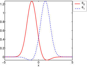
Figure 3: From even and odd parity modes of a double-well potential, one can construct the left $\phi_{0}$ and right $\phi_{1}$ localized Wannier states of the system.

If this approximate field is substituted in the Hamiltonian, Eq. (3.1), we can exploit the orthogonality of the wave functions and obtain the two-body matrix elements $\phi_{ijkl}$

$$\delta_{ij}=\int_{-\infty}^{\infty}{\rm d}x\,\phi_{i}(x)\phi_{j}(x),\quad\phi_{ijkl}=\int_{-\infty}^{\infty}{\rm d}x\,\phi_{i}(x)\phi_{j}(x)\phi_{k}(x)\phi_{l}(x).$$ (18)

Out of the sixteen combinations for $\phi_{ijkl}$, we only retain the physically most relevant contributions and disregard others deliberately. This leads to the following model Hamiltonian for two coupled Josephson junctions

$$\hat{H} = \Lambda(\hat{e}_{0}^{{\dagger}}\hat{e}_{1}^{\phantom{{\dagger}}}+\hat{e}_{1}^{{\dagger}}\hat{e}_{0}^{\phantom{{\dagger}}}+\hat{g}_{0}^{{\dagger}}\hat{g}_{1}^{\phantom{{\dagger}}}+\hat{g}_{1}^{{\dagger}}\hat{g}_{0}^{\phantom{{\dagger}}})$$

$$+ \delta(\hat{e}_{0}^{{\dagger}}\hat{e}_{0}^{\phantom{{\dagger}}}-\hat{g}_{0}^{{\dagger}}\hat{g}_{0}^{\phantom{{\dagger}}})+\delta(\hat{e}_{1}^{{\dagger}}\hat{e}_{1}^{\phantom{{\dagger}}}-\hat{g}_{1}^{{\dagger}}\hat{g}_{1}^{\phantom{{\dagger}}})$$

$$+ \Omega_{0}(\hat{e}_{0}^{{\dagger}}\hat{g}_{0}^{\phantom{{\dagger}}}+\hat{g}_{0}^{{\dagger}}\hat{e}_{0}^{\phantom{{\dagger}}})+\Omega_{1}(\hat{e}_{1}^{{\dagger}}\hat{g}_{1}^{\phantom{{\dagger}}}+\hat{g}_{1}^{{\dagger}}\hat{e}_{1}^{\phantom{{\dagger}}})$$

$$+ g(\hat{e}_{0}^{{\dagger}}\hat{e}_{0}^{{\dagger}}\hat{e}_{0}^{\phantom{{\dagger}}}\hat{e}_{0}^{\phantom{{\dagger}}}+\hat{g}_{0}^{{\dagger}}\hat{g}_{0}^{{\dagger}}\hat{g}_{0}^{\phantom{{\dagger}}}\hat{g}_{0}^{\phantom{{\dagger}}}+\hat{e}_{1}^{{\dagger}}\hat{e}_{1}^{{\dagger}}\hat{e}_{1}^{\phantom{{\dagger}}}\hat{e}_{1}^{\phantom{{\dagger}}}+\hat{g}_{1}^{{\dagger}}\hat{g}_{1}^{{\dagger}}\hat{g}_{1}^{\phantom{{\dagger}}}\hat{g}_{1}^{\phantom{{\dagger}}})$$

where all coupling constants are implicitly rescaled by the corresponding single particle or two-body matrix elements and the new parameter $\Lambda$ measures the spatial hopping rate between the sites.

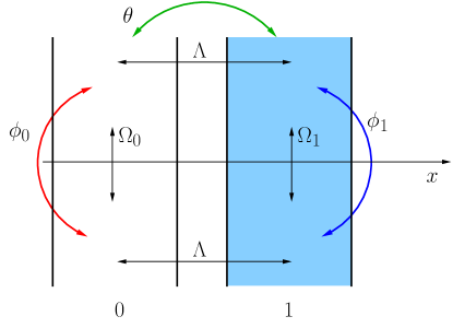
Figure 4: Coupling pattern of two coupled Josephson junctions $JJ_{0}$ and $JJ_{1}$ with, $\Omega_{1}=-\Omega_{0}$. The classical phase $\theta$ refers to a particle current between the spatial sites, while the phases $\phi_{0}$ and $\phi_{1}$ are currents within the two-state atoms.

3.4 Fock-space representation of the four mode model

In principle, it is possible to solve the four-mode Schrödinger equation in Fock space by projecting it on the $N$-particle sector

$$|{\psi,N}\rangle=\delta(\hat{N}-N)\sum_{\mathbf{n}=0}^{\infty}\psi_{\mathbf{n}}|{\mathbf{n}=(n_{0}^{e},n_{0}^{g},n_{1}^{e},n_{1}^{g})}\rangle.$$ (21)

The number constraint on the state remains valid throughout the time-evolution as number conservation is encoded into our Hamiltonian from the beginning in Eq. (10). This reduces the discrete $d=4$ dimensional eigenvalue problem to an effective three-dimensional problem with nontrivial boundaries. We have illustrated the finite support of the amplitude field $\psi_{\mathbf{n}}$ in Fig. 5. It is a $(d-1)$-dimensional simplex embedded into a $d$-dimensional Fock space. The full analysis of this problem is an interesting problem in its own right and will be presented in a forthcoming publication.

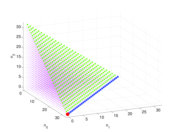
Figure 5: A three dimensional simplex represents the four-mode Fock space for $N=32$ particles. The axes are labeled in a generic lexicographical order $(n_{0},n_{1},n_{2})$ and implicitly $n_{4}=N-n_{0}-n_{1}-n_{2}$.

3.5 The classical limit of the four mode model

It is not necessary to solve the four-mode problem in Fock-space to understand the principal features of the equilibrium configuration. Thus, we will again resort to the classical approximation and use the number-symmetry broken coherent state approximation for the quantum state

$$|{\psi}\rangle = |{\boldsymbol{\alpha}=(e_{0},g_{0},e_{1},g_{1})^{\top}}\rangle,\quad\hat{e}_{i}|{\psi}\rangle=e_{i}|{\psi}\rangle,\quad\hat{g}_{i}|{\psi}\rangle=g_{i}|{\psi}\rangle.$$ (22)

The dynamics is simply obtained from the Lagrangian

$$\mathcal{L}(\boldsymbol{\alpha},\dot{\boldsymbol{\alpha}}) = \langle{\boldsymbol{\alpha}}|i\partial_{t}-\hat{H}|{\boldsymbol{\alpha}}\rangle=i\boldsymbol{\alpha}^{\ast}\dot{\boldsymbol{\alpha}}-\mathcal{H}(\boldsymbol{\alpha},\boldsymbol{\alpha}^{\ast})-\frac{i}{2}\frac{d}{dt}\mathcal{N}(\boldsymbol{\alpha},\boldsymbol{\alpha}^{\ast}),$$ (23)

if we introduce the classical Hamilton functions $\mathcal{H}(\boldsymbol{\alpha},\boldsymbol{\alpha}^{\ast})=\langle{\boldsymbol{\alpha}}|\hat{H}|{\boldsymbol{\alpha}}\rangle$ and number expectation values $\mathcal{N}(\boldsymbol{\alpha},\boldsymbol{\alpha}^{\ast})=\langle{\boldsymbol{\alpha}}|\hat{N}|{\boldsymbol{\alpha}}\rangle$, as

$$\mathcal{H}(\boldsymbol{\alpha},\boldsymbol{\alpha}^{\ast}) = \Lambda\left(e_{0}^{\ast}e_{1}+e_{1}^{\ast}e_{0}+g_{0}^{\ast}g_{1}+g_{1}^{\ast}g_{0}\right)$$

$$+ \delta_{0}\left(|e_{0}|^{2}-|g_{0}|^{2}\right)+\delta_{1}\left(|e_{1}|^{2}-|g_{1}|^{2}\right)$$

$$+ \Omega_{0}\left(e_{0}^{\ast}g_{0}+g_{0}^{\ast}e_{0}\right)+\Omega_{1}\left(e_{1}^{\ast}g_{1}+g_{1}^{\ast}e_{1}\right)$$

$$+ g(|e_{0}|^{4}+|g_{0}|^{4}+|e_{1}|^{4}+|g_{1}|^{4}),$$

$$\mathcal{N}(\boldsymbol{\alpha},\boldsymbol{\alpha}^{\ast}) = |e_{0}|^{2}+|g_{0}|^{2}+|e_{1}|^{2}+|g_{1}|^{2}.$$ (25)

If the dynamical coordinate is $\boldsymbol{\alpha}$, then we find the canonical momentum as

$$\pi_{k}=\frac{\partial\mathcal{L}}{\partial\dot{\alpha}_{k}}=i\alpha_{k}^{\ast},$$ (26)

Consequently, variables and momenta obey the Poisson bracket $\left\{\alpha_{j},\pi_{k}\right\}=\delta_{jk}$. By construction, number conservation is satisfied dynamically as

$$\frac{d}{dt}\mathcal{N}=\left\{\mathcal{H},\mathcal{N}\right\}=0$$ (27)

and the Hamilton equations of motion for the coordinates read

$$\frac{d}{dt}\boldsymbol{\alpha}=\left\{\mathcal{H},\boldsymbol{\alpha}\right\}=-i\mathcal{K}\boldsymbol{\alpha}$$ (28)

$$\mathcal{K}=\left(\begin{array}[]{cccc}\delta_{0}+2g|\alpha_{0}|^{2}&\Omega_{0}&\Lambda&0\\ \Omega_{0}&-\delta_{0}+2g|\alpha_{1}|^{2}&0&\Lambda\\ \Lambda&0&\delta_{1}+2g|\alpha_{2}|^{2}&\Omega_{1}\\ 0&\Lambda&\Omega_{1}&-\delta_{1}+2g|\alpha_{3}|^{2}\end{array}\right).$$ (33)

In classical mechanics, we can deliberately choose new coordinates and momenta to accounts for symmetries of the Hamiltonian. If a new variable of a canonical transformation matches a conserved quantity, it follows that the conjugate variable becomes cyclic. In this spirit, we will introduce the following pairs of action-angle variables: $(\Phi,\mathcal{N})$ measures the global phase and the total particle number $\mathcal{N}=n_{0}^{g}+n_{0}^{e}+n_{1}^{g}+n_{1}^{e}$ of the system, $(\theta,\mathcal{M})$ measures the relative phase between left and right sites and the population imbalance $\mathcal{M}=n_{0}^{e}+n_{0}^{g}-(n_{1}^{e}+n_{1}^{g})$ inbetween, $(\phi_{0},\mathcal{M}_{0}=n_{0}^{e}-n_{0}^{g})$, and $(\phi_{1},\mathcal{M}_{1}=n_{1}^{e}-n_{1}^{g})$ measure the relative internal phase of the atoms on each site and the corresponding population difference. This coupling scheme for the phases and population imbalances has been illustrated in Fig. 4. By inverting the population relations, one finds the individual occupation number $n_{l}^{\sigma}$ per site as

$$\begin{array}[]{ll}n_{0}^{e}=\frac{1}{4}(\mathcal{N}+\mathcal{M}+2\mathcal{M}_{0}),&n_{0}^{g}=\frac{1}{4}(\mathcal{N}+\mathcal{M}-2\mathcal{M}_{0}),\\ n_{1}^{e}=\frac{1}{4}(\mathcal{N}-\mathcal{M}+2\mathcal{M}_{1}),&n_{1}^{g}=\frac{1}{4}(\mathcal{N}-\mathcal{M}-2\mathcal{M}_{1}),\end{array}$$ (36)

Finally, we can use these physical coordinates in a canonical transformation from complex amplitudes to real action-angle variables

$$e_{0} = e^{-i(\Phi+\theta+\phi_{0})}\sqrt{n_{0}^{e}},\quad g_{0}=e^{-i(\Phi+\theta-\phi_{0})}\sqrt{n_{0}^{g}}$$ (37)

$$e_{1} = e^{-i(\Phi-\theta+\phi_{1})}\sqrt{n_{1}^{e}},\quad g_{1}=e^{-i(\Phi-\theta-\phi_{1})}\sqrt{n_{1}^{g}}.$$

For later use it is also useful to introduce the auxiliary phases $\theta_{i}$, which are global phases of the subsystem on site i:

$$\theta_{0}=\Phi+\theta,\quad\theta_{1}=\Phi-\theta.$$ (38)

By substituting field amplitudes into the Lagrangian of Eq. (23), one can again identify the variables and corresponding canonical momenta as

$$\frac{\partial\mathcal{L}}{\partial\dot{\Phi}}=\mathcal{N},\quad\frac{\partial\mathcal{L}}{\partial\dot{\theta}}=\mathcal{M},\quad\frac{\partial\mathcal{L}}{\partial\dot{\phi}_{0}}=\mathcal{M}_{0},\quad\frac{\partial\mathcal{L}}{\partial\dot{\phi}_{1}}=\mathcal{M}_{1}.$$ (39)

With this new coordinates and momenta we obtain a Hamilton function

$$\mathcal{H}^{\prime} = \mathcal{H}^{\prime}(\theta,\phi_{0},\phi_{1},\mathcal{N},\mathcal{M},\mathcal{M}_{0},\mathcal{M}_{1})$$

$$= \frac{\Lambda}{2}\cos{(2\theta+\phi_{0}-\phi_{1})}\sqrt{(\mathcal{N}+\mathcal{M}+2\mathcal{M}_{0})(\mathcal{N}-\mathcal{M}+2\mathcal{M}_{1})}$$

$$+ \frac{\Lambda}{2}\cos{(2\theta-\phi_{0}+\phi_{1})}\sqrt{(\mathcal{N}+\mathcal{M}-2\mathcal{M}_{0})(\mathcal{N}-\mathcal{M}-2\mathcal{M}_{1})}$$

$$+ \Omega_{0}\cos{(2\phi_{0})}\sqrt{(\mathcal{N}+\mathcal{M})^{2}/4-\mathcal{M}_{0}^{2}}+\delta_{0}\mathcal{M}_{0}+\delta_{1}\mathcal{M}_{1}$$

$$+ \Omega_{1}\cos{(2\phi_{1})}\sqrt{(\mathcal{N}-\mathcal{M})^{2}/4-\mathcal{M}_{1}^{2}}+\frac{g}{4}\left(\mathcal{N}^{2}+\mathcal{M}^{2}+2\mathcal{M}_{0}^{2}+2\mathcal{M}_{1}^{2}\right).$$

For the parameters $\delta=1$, $\Omega_{0}=1$, $\Omega_{1}=-1$, $\Lambda=0.1$, $g=0.005$, $\mathcal{N}=100$, we have numerically minimized the energy of Eq. (3.5) and find two minima $E=E_{0},E_{1}$. Please note that the amplitudes of the solutions $\boldsymbol{\alpha}$ are real valued. Due to the invariance of the solutions under global phase change, we can deliberately modify them and choose the global phase of the left site as the common ground $\theta_{0}=0$. In Tab. 1, we have listed the energies, the real valued amplitudes and the phases calculated according Eqs. (37) and (38).

Table 1: Two stationary solutions of the Hamilton equation, energies $E_{0},E_{1}$, field amplitudes $\boldsymbol{\alpha}=(e_{0},g_{0},e_{1},g_{1})$ and phases. The global phase of the left site, i.e., $\theta_{0}=0$ was chosen as the common ground.

• $E$	$e_{0}$	$g_{0}$	$e_{1}$	$g_{1}$	$\Phi$	$\phi_{0}$	$\phi_{1}$	$\theta$	$\theta_{0}$	$\theta_{1}$
  $-129.84$	$2.82$	$-6.48$	$2.82$	$6.48$	$\frac{\pi}{4}$	$\frac{\pi}{2}$	0	$-\frac{\pi}{4}$	0	$\frac{\pi}{2}$
  $-117.00$	$3.16$	$-6.32$	$-3.16$	$-6.32$	$-\frac{\pi}{4}$	$\frac{\pi}{2}$	0	$\frac{\pi}{4}$	0	$-\frac{\pi}{2}$

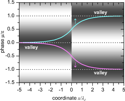
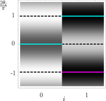
Figure 6: Comparing a spatially extended $0$-$\pi$-junction in a superconductor (left panel) calculated according to the sine-Gordon equation [61] to an analog, two site junction in an atomic BEC (right panel). We have plotted the scaled global phase $\theta_{i}$ vs. the site index $i=0,1$.

4 Conclusion and Perspectives

In the present article we have briefly summarized the status of the fluxon and semifluxon physics in superconductivity. In particular, we were focusing on an effect that exists in a long $0$-$\pi$ geometry where two Josephson junctions were in the groundstate and one obtains a Josephson vortex of fractional magnetic flux, pinned at the $0$-$\pi$ boundary. Depending on the preparation procedure, this “classical” state of the superconducting device can occur in two different configurations: with the magnetic flux equal to $+\Phi_{0}/2$ or $-\Phi_{0}/2$.

This arrangement of superconducting junctions has been analyzed and transfered to the context of an atomic bosonic quantum gas, where two-state atoms in a double well trap are coupled in a similar fashion. There, the optical $0$-$\pi$ junction is represented by the left/right localized internal atomic Josephson junctions and a jumping phase of the complex-valued Rabi-frequency. We have derived a simple four-mode model for this case and showed that in the “classical” approximation it qualitatively resembles the semifluxons seen in superconductivity.

In the superconducting case, one observes a smooth spatial behaviour of the phase across the $0$-$\pi$ boundary. In the atomic case, this will emerge also by a more realistic modeling for the Rabi-frequency and spatial motion. This is currently under investigation. Eventually, the four-mode, $0$-$\pi$ Josephson model will be also instrumental in examining the quantum properties of these macroscopic semifluxon states and we will explore the macroscopic tunneling between them [61]. This is also work in progress and will be reported in a forthcoming publication.

References

References

- [1] Arimondo E, Phillips WD, Strumia F, editors. Laser Manipulation of Atoms and Ions. North-Holland; 1992.
- [2] Pitaevskii L, Stringari S. Bose-Einstein Condensation. Oxford: Claredon Press; 2003.
- [3] Buckel W, Kleiner R. Superconductivity: Fundamentals and Applications. 2nd ed. Wiley-VCH; 2004.
- [4] Folman R, Krüger P, Schmiedmayer J, Denschlag J, Henkel C. Mircoscopic atom optics: From wires to an atom chip. Adv At Mol Opt Phys. 2002;48:263.
- [5] Fortágh J, Zimmermann C. Magnetic microtraps for ultracold atoms. Rev Mod Phys. 2007;79:235. And Refs. therein.
- [6] Du S, Squires M, Imai Y, Czaia L, Saravanan R, Bright V, et al. Atom-chip Bose-Einstein condensation in a portable vacuum cell. Phys Rev A. 2004;70:53606.
- [7] Vogel A, Schmidt M, Sengstock K, Bongs K, Lewoczko W, Schuldt T, et al. Bose-Einstein condensates in microgravity. Appl Phys B. 2006;84:664.
- [8] Nandi G, Walser R, Kajari E, Schleich WP. Dropping cold quantum gases on Earth over long times and large distances. Phys Rev A. 2007;76:63617.
- [9] Könemann T, Brinkmann W, Göklü E, Lämmerzahl C, Dittus H, van Zoest T, et al. First Realization of a magneto-optical trap in weightlessness. Appl Phys B. 2007;89:431.
- [10] Likharev K. Superconducting weak links. Rev Mod Phys. 1979;51:101.
- [11] Barone A, Paterno G. Physics and Application of the Josephson Effect. New York: Wiley Interscience; 1982.
- [12] Makhlin Y, Schön G, Shnirman A. Quantum-state engineering with Josephson-junction devices. Rev Mod Phys. 2001;73:357.
- [13] Castin Y, Dalibard J. Relative phase of two Bose-Einstein condensates. Phys Rev A. 1997;55:4330.
- [14] Andrews M, Townsend C, Miesner HJ, Durfee D, Kurn D, Ketterle W. Observation of Interference Between Two Bose Condensates. Science. 1997;275:637.
- [15] Ketterle W, Durfee D, Stamper-Kurn D. Making, probing and understanding Bose-Einstein condensates. In: Inguscio M, Stringari S, Wieman C, editors. Proceedings of the International School of Physics ”Enrico Fermi”, Course CXL. Soc. Italiana di Fisica,Bologna, Italy. Amsterdam: IOS Press; 1999. .
- [16] Anderson BP, Kasevich MA. Macroscopic Quantum Interference from Atomic Tunnel Arrays. Science. 1998 Nov;282:1686.
- [17] Zapata I, Sols F, Leggett T. Josephson effect between trapped Bose-Einstein condensates. Phys Rev A. 1998;57:R28.
- [18] Williams J, Walser R, Cooper J, Cornell E, Holland M. Nonlinear Josephson-type oscillations of a driven, two-component Bose-Einstein condensate. Phys Rev A, Rapid Comm. 1999;59:31.
- [19] Williams J, Walser R, Cooper J, Cornell E, Holland M. Excitation of a dipole topological state in a strongly coupled two-component Bose-Einstein condensate. Phys Rev A. 2000;61:033612.
- [20] Leggett A. Bose-Einstein condensation in the alkali gases: Some fundamental concepts. Rev Mod Phys. 2001;73:307.
- [21] Giovanazzi S, Smerzi A, Fantoni S. Josephson Effects in Dilute Bose-Einstein Condensates. Phys Rev Lett. 2000;84:4521.
- [22] Albiez M, Gati R, Fölling J, Hunsmann S, Cristian M, Oberthaler MK. Direct observation of tunneling and nonlinear self-trapping in a single bosonic Josephson junction. Phys Rev Lett. 2005;95:010402.
- [23] Gati R, Oberthaler M. A bosonic Josephson junction. J Phys B: At Mol Opt Phys. 2007;40:R61.
- [24] Cataliotti F, Burger S, Fort C, Maddaloni P, Minardi F, Trombettoni A, et al. Josephson junction arrays with Bose-Einstein condensates. Science. 2001;293:843.
- [25] Nandi G, Sizman A, Fortágh J, Walser R. A numberfilter for matterwaves. arXiv: 07101737. 2007;.
- [26] Bloch I. Ultracold quantum gases in optical lattices. Nature Physics. 2005;1:23.
- [27] Fölling S, Trotzky S, Cheinet P, Feld M, Saers R, Widera1 A, et al. Direct observation of second-order atom tunnelling. Nature. 2007;448:1029.
- [28] Hadzibabic Z, Stock S, Battelier B, Bretin V, Dalibard J. Interference of an array of independent Bose-Einstein condensates. Phys Rev Lett. 2004;93:180403.
- [29] Kaurov VM, Kuklov AB. Atomic Josephson vortices. Phys Rev A. 2006;73(1):013627.
- [30] Kaurov VM, Kuklov AB. Josephson vortex between two atomic Bose-Einstein condensates. Phys Rev A. 2005;71(1):011601.
- [31] Goldobin E, Koelle D, Kleiner R. Semifluxons in long Josephson 0--junctions. Phys Rev B. 2002;66:100508(R).
- [32] Kleiner R, Steinmeyer F, Kunkel G, Müller P. Intrinsic Josephson effects in Bi2Sr2CaCu2O8 single crystals. Phys Rev Lett. 1992 Apr;68(15):2394–2397.
- [33] Kleiner R, Müller P. Intrinsic Josephson effects in high- superconductors. Phys Rev B. 1994 Jan;49(2):1327–1341.
- [34] Ryazanov VV, Oboznov VA, Rusanov AY, Veretennikov AV, Golubov AA, Aarts J. Coupling of Two Superconductors through a Ferromagnet: Evidence for a Junction. Phys Rev Lett. 2001;86:2427.
- [35] Blum Y, Tsukernik A, Karpovski M, Palevski A. Oscillations of the Superconducting Critical Current in Nb-Cu-Ni-Cu-Nb Junctions. Phys Rev Lett. 2002;89:187004.
- [36] Bauer A, Bentner J, Aprili M, Della-Rocca ML, Reinwald M, Wegscheider W, et al. Spontaneous Supercurrent Induced by Ferromagnetic Junctions. Phys Rev Lett. 2004;92(21):217001.
- [37] Sellier H, Baraduc C, Lefloch F, Calemczuk R. Half-Integer Shapiro Steps at the - Crossover of a Ferromagnetic Josephson Junction. Phys Rev Lett. 2004;92(25):257005.
- [38] Oboznov VA, Bol’ginov VV, Feofanov AK, Ryazanov VV, Buzdin AI. Thickness Dependence of the Josephson Ground States of Superconductor-Ferromagnet-Superconductor Junctions. Phys Rev Lett. 2006;96(19):197003.
- [39] Kontos T, Aprili M, Lesueur J, Genêt F, Stephanidis B, Boursier R. Josephson Junction through a Thin Ferromagnetic Layer: Negative Coupling. Phys Rev Lett. 2002;89:137007.
- [40] Weides M, Kemmler M, Goldobin E, Koelle D, Kleiner R, Kohlstedt H, et al. High quality ferromagnetic 0 and Josephson tunnel junctions. Appl Phys Lett. 2006;89(12):122511.
- [41] Vavra O, Gazi S, Golubovic DS, Vavra I, Derer J, Verbeeck J, et al. 0 and phase Josephson coupling through an insulating barrier with magnetic impurities. Phys Rev B. 2006;74(2):020502.
- [42] Cleuziou JP, Wernsdorfer W, Bouchiat V, Ondarcuhu T, Monthioux M. Carbon nanotube superconducting quantum interference device. Nature Nanotech. 2006;1(1):53–59.
- [43] van Dam JA, Nazarov YV, Bakkers EPAM, De Franceschi S, Kouwenhoven LP. Supercurrent reversal in quantum dots. Nature (London). 2006;442(7103):667–670.
- [44] Bulaevskiĭ LN, Kuziĭ VV, Sobyanin AA. Superconducting system with weak coupling to the current in the ground state. JETP Lett. 1977;25(7):290–294. [Pis’ma Zh. Eksp. Teor. Fiz. 25, 314 (1977)].
- [45] Bulaevskii LN, Kuzii VV, Sobyanin AA. On Possibility of the Spontaneous Magnetic Flux in a Josephson junction containing magnetic impurities. Solid State Commun. 1978;25:1053–1057.
- [46] Xu JH, Miller JH, Ting CS. -vortex state in a long 0--Josephson junction. Phys Rev B. 1995;51:11958.
- [47] Kirtley JR, Tsuei CC, Moler KA. Temperature Dependence of The Half-Integer Magnetic Flux quantum. Science. 1999;285:1373.
- [48] Kirtley JR, Tsuei CC, Rupp M, Sun JZ, Yu-Jahnes LS, Gupta A, et al. Direct imaging of integer and half-integer Josephson vortices in high- grain boundaries. Phys Rev Lett. 1996;76:1336.
- [49] Smilde HJH, Ariando, Blank DHA, Gerritsma GJ, Hilgenkamp H, Rogalla H. -Wave-Induced Josephson Current Counterflow in YBa2Cu3O7/Nb Zigzag Junctions. Phys Rev Lett. 2002;88:057004.
- [50] Ariando, Darminto D, Smilde HJH, Leca V, Blank DHA, Rogalla H, et al. Phase-Sensitive Order Parameter Symmetry Test Experiments Utilizing Nd2-xCexCuO4-y/Nb Zigzag Junctions. Phys Rev Lett. 2005;94(16):167001.
- [51] Hilgenkamp H, Ariando, Smilde HJH, Blank DHA, Rijnders G, Rogalla H, et al. Ordering and manipulation of the magnetic moments in large-scale superconducting -loop arrays. Nature (London). 2003;422:50–53.
- [52] Kirtley JR, Tsuei CC, Ariando, Smilde HJH, Hilgenkamp H. Antiferromagnetic ordering in arrays of superconducting -rings. Phys Rev B. 2005;72(21):214521.
- [53] Kogan VG, Clem JR, Kirtley JR. Josephson vortices at tricrystal boundaries. Phys Rev B. 2000;61(13):9122–9129.
- [54] Zenchuk A, Goldobin E. Analytical analysis of ground states of 0- long Josephson junctions. Phys Rev B. 2004;69:024515.
- [55] Susanto H, van Gils SA, Visser TPP, Ariando, Smilde HJH, Hilgenkamp H. Static semifluxons in a long Josephson junction with -discontinuity points. Phys Rev B. 2003;68:104501.
- [56] Kirtley JR, Moler KA, Scalapino DJ. Spontaneous flux and magnetic-interference patterns in 0- Josephson junctions. Phys Rev B. 1997;56:886.
- [57] Goldobin E, Stefanakis N, Koelle D, Kleiner R. Fluxon-semifluxon interaction in an annular long Josephson - junction. Phys Rev B. 2004;70(9):094520.
- [58] Lazarides N. Critical current and fluxon dynamics in overdamped 0- Josephson junctions. Phys Rev B. 2004;69(21):212501.
- [59] Goldobin E, Koelle D, Kleiner R. Ground state and bias current induced rearrangement of semifluxons in 0--Josephson junctions. Phys Rev B. 2003;67:224515.
- [60] Susanto H, Goldobin E, Koelle D, Kleiner R, van Gils SA. Controllable plasma energy bands in a one-dimensional crystal of fractional Josephson vortices. Phys Rev B. 2005;71(17):174510.
- [61] Goldobin E, Vogel K, Crasser O, Walser R, Schleich WP, Koelle D, et al. Quantum tunneling of semifluxons in a -- long Josephson junction. Phys Rev B. 2005;72(5):054527.
- [62] Schleich WP. Quantum Optics in Phase Space. Berlin, Germany: Wiley-VCH; 2001.
- [63] Feynman RP, Hibbs AH. Quantum mechanics and path integrals. McGraw-Hill; 1965.