Characteristics of the asymmetric simple exclusion process in the presence of
quenched spatial disorder

Abstract

We investigate the effect of quenched spatial disordered hopping rates on the characteristics of the asymmetric simple exclusion process (ASEP) with open boundaries both numerically and by extensive simulations. Disorder averages of the bulk density and current are obtained in terms of various input and output rates. We study the binary and uniform distributions of disorder. It is verified that the effect of spatial inhomogeneity is generically to enlarge the size of the maximal current phase. This is in accordance with the mean field results obtained by Harris and Stinchcombe stinchcombe . Furthermore, we obtain the dependence of the current and the bulk density on the characteristics of the disorder distribution function. It is shown that the impact of disorder crucially depends on the particle input and out rates. In some situations, disorder can constructively enhance the current.

I Introduction

Transport processes in disordered media constitute an important class of problems especially in the light of their relevance to the modelling of a vast variety of phenomena in physics and many interdisciplinary areas. A partial list of applications includes transport phenomena in porous media, diffusion in biological tissues and conduction through composite solids sahimi ; bunde ; hughes . It is a well-established fact the disorder can strongly affect the transport characteristics of equilibrium as well as out of equilibrium systems. Among various non equilibrium systems, low dimensional driven lattice gases have played an important role in describing the transport in many physical, chemical and biological processes ligget ; zia ; schutz1 ; css99 ; hinrischsen . In particular, one dimensional driven diffusive systems in the absence of disorder have been extensively studied during the past two decades and at present there exists a rich literature of results both analytic and numeric schutz1 . Phase structures of these systems are well known. It is well understood that non-equilibrium systems can exhibit phase transitions in low dimensions. A model which has played a paradigmatic role in out of equilibrium statistical physics is the asymmetric simple exclusion process (ASEP) mcdonald . The model is amenable to exact analytical solution derida1 ; domany ; derida2 . Therefore it is a natural and important question to investigate the effect of quenched disorder on the phase structure of ASEP. Recently some efforts and new strides have been made in the challenge between disorder, interaction and drive. The exploration of the disordered ASEP began with a single defective site in a periodic chain by Janowsky and Lebowitz lebowitz1 ; lebowitz2 . They showed that even one defective site can remarkably lead to global effects on the system current and density profile. Evans solved the ASEP with moving impurities where particle hopping rates were chosen randomly from a distribution function evans1 . It was shown that special distribution functions can give rise to a new phase transition analogous to Bose condensation. Subsequently, Tripathy and Barma barma1 ; barma2 considered the ASEP on a ring with many defective sites. Their investigation revealed the existence of phase segregation in a wide range of global densities in the chain. In conjunction with the results of the ASEP on a ring, an investigation of the disordered ASEP in an open chain was introduced by Kolomeisky kolomeisky1 . He showed that in some ranges of input and output rates, a single defect in the bulk could affect the system properties on a global scale. Recently a new wave of attention has been created on the disordered ASEPkrug ; kolwanker ; derida3 ; stinchcombe ; chou ; shaw1 ; shaw2 ; lakatos1 ; santen ; lakatos2 . In particular, Chou and Lakatos have studied the effect of a few defective sites in the open ASEP chou . Their investigations have revealed that generically the disorder’s impact is highest when the number of defects is very small. Increasing the number of defects above a certain value has no further effect on the system current. The question of the effect of a single defect in the ASEP coupled with a 3D bulk reservoir with adsorption/desorption kinetics was recently addressed by Frey frey . Besides, some time-dependent aspects of the disordered ASEP has been discussed by Barma barma3 . Our goal in this paper is to deal in some more depth with the problem of the disordered ASEP. Especially we will focus on the role of the binary distribution function where it provides the possibility of simultaneous study of both the strength and the density of disorder throughout the chain. Via extensive MC simulations, we show for the binary and uniform distribution functions the generic impact of disorder is to reduce the size of the low and high density phases. More interestingly, we show in some circumstances, disorder can constructively act in a manner to increase the system current.

II Description of the Problem and numerical solution

To keep the paper self-contained, let us first define the disordered ASEP. Imagine a one dimensional stochastic process defined on a discrete 1D lattice of length $L$. Each site can hold at most one particle. We assign an integer valued number $s_{i}$ to each site $i$ (see figure (1) ). If site $i$ is occupied, $s_{i}$=1. If it is empty then $s_{i}$ is zero. The system configuration at each time $t$ is characterized by specifying the occupation numbers $s_{i}~{}~{}i=1,\cdots,L$. During an infinitesimal time $dt$ each particle can stochastically hop to its rightmost neighbouring site provided the target site is empty. If the target site is already occupied by another particle, the attempted movement is rejected. The hopping takes place with a site dependent rate $p_{i}$ which is drawn from a given distribution function $f(p)$.

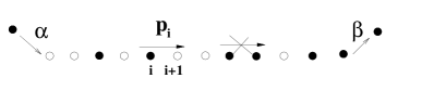
Figure 1: Asymmetric exclusion process with spatial disorder.

There is no spatial correlation between the set $p_{i}~{}~{}i=1,\cdots,L$ and correspondingly the $p_{i}$’s can be regarded as independent stochastic variables which are identically distributed according to the site independent distribution function $f(p)$. Denoting the averaged local density at site $i$ by $n_{i}$, one can simply write the following rate equations for a particular realisation of hopping rates $p_{1},\cdots,p_{L}~{}(i=2,\cdots,L-1)$:

$$\frac{d}{dt}\langle n_{i}\rangle=p_{i-1}\langle n_{i-1}(1-n_{i})\rangle-p_{i}\langle n_{i}(1-n_{i+1})\rangle,$$ (1)

$$\frac{d}{dt}\langle n_{1}\rangle=\alpha(1-\langle n_{1}\rangle)-p_{1}\langle n_{1}(1-n_{2})\rangle,$$ (2)

$$\frac{d}{dt}\langle n_{L}\rangle=p_{L-1}\langle n_{L-1}(1-n_{L})\rangle-\beta\langle n_{L}\rangle.$$ (3)

No exact analytical solution exists for the above set of nonlinear differential equations. Restricting ourselves to the stationary state properties of the system, we set the left hand sides equal to zero. We further simplify the equations by taking the assumption of a mean field equation where the two-point functions are replaced by the product of two one-point functions. This assumption reduces the steady state equations into a set of nonlinear algebraic equation with $L$ unknowns $n_{1},n_{2},\cdots,n_{L}$.

II.1 Numerical approach to mean field equations

Even by employing the assumption of a mean field, we are not able to solve the nonlinear algebraic equations. Therefore, we should resort to numerical methods. We now outline a numerical approach for solving the set of nonlinear equations. The approach is based on the shooting method for solving boundary value problems. To this end, we choose a trial $n_{1}$ denoted by $n_{1}^{tr}$ and successively evaluate $n_{2},\cdots,n_{L}$ through forward iteration. The system current then turns out to be $\alpha(1-n_{1}^{tr})$. Since the current should be equal for all sites, if the guessed value of $n_{1}^{tr}$ was correct then the current evaluated from the last site i.e., $\beta n_{L}$ would have the same amount $\alpha(1-n_{1}^{tr})$ evaluated from the first site. To match these currents, we gradually increase $n_{1}^{tr}$ from zero and evaluate both currents from the first and last sites. Whenever these two values become equal, then we have a solution. Note that in an acceptable solution, all the densities $\langle n_{1}\rangle,\cdots,\langle n_{L}\rangle$ should lie between $0$ and $1$. We are interested in knowing the overall effect of disorder on the transport characteristics of the ASEP. For given values of $\alpha$ and $\beta$, we evaluate the current and density for many samples of disordered chains and average over these samples. We denote the sample averaged current and bulk density by $\langle J\rangle$ and $\langle\rho\rangle$ respectively. For obtaining a better insight, we have also executed extensive Monte Carlo simulations. The disorder distributions we consider consist of uniform and binary. More explicitly, the normalized uniform distribution in the interval $[a,b]$ has the functional form $f_{1}(p)=\frac{1}{b-a}$ with mean $\frac{a+b}{2}$ and variance $\frac{(b-a)^{2}}{12}$. The binary distribution has the form $f_{2}(p)=f\delta(p-p_{1})+(1-f)\delta(p-p_{2})$ where the binary rates $p_{1}$ and $p_{2}$ and their probabilities $f$ and $1-f$ are given. The mean value and the variance are $fp_{1}+(1-f)p_{2}$ and $fp_{1}^{2}+(1-f)p_{2}^{2}-[fp_{1}+(1-f)p_{2}]^{2}$ respectively. In the subsequent sections, we show the result of simulation as well as numerical solution of the mean field equations.

III Binary distribution function

Let us first discuss the binary distribution of the quenched disorder. Although in this type of distribution the defect strength is allowed to take only an integer number of values (here $2$), but even in this simple case one encounters some nontrivial aspects which are worth investigating. Figure (2) depicts the dependence of average current versus $\beta$ for some fixed $\alpha$. The parameters of the binary distribution function is as follows: $f=0.5,~{}p_{1}=0.8$ and $p_{2}=1.2$. The mean value of the quenched hopping rate is fixed at $1$. The bulk density and the current have been averaged over $1000$ disordered samples and the system size is $200$.

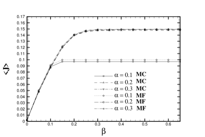
Figure 2: $\langle J\rangle$ versus $\beta$ for various input rates $\alpha$.

One observes similar behaviour to the normal ASEP. Currents rise up to a critical $\beta$ and then get saturated. The overall effect of disorder is to reduce the value of the currents in each phase. In the normal ASEP, the dependence of current on $\beta$ in the high density (HD) phase is $\beta(1-\beta)$. Saturation of current means that we are in the maximal current (MC) phase. However, the current saturates at 0.15 which is less than the value of the maximal current 0.25 in the normal ASEP. The reason is due to the presence of defects which slow down the current. Figure (3) exhibits the dependence of $\langle J\rangle$ versus the input rate $\alpha$.

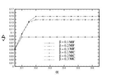
Figure 3: Disorder-averaged current vs $\alpha$ for various output rates $\beta$. System size is 200.

The behaviour seen in the above graph is analogous to the normal ASEP with the difference that the disorder has yielded to an overall diminishing of $\langle J\rangle$. In the normal ASEP, the dependence of $\langle J\rangle$ on $\alpha$ in the low density phase is $\alpha(1-\alpha)$. We note that upon entering the saturation regime i.e., the MC phase, the current value which is 0.15, is less than that of the normal ASEP 0.25. The dependence of bulk densities on $\alpha$ and $\beta$ are exhibited in figures (4,5). Similar to current diagrams, the overall behaviour is analogous to the normal ASEP. Here the effect of disorder is to enhance the densities.

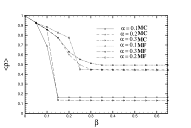
Figure 4: Disorder-averaged densities vs $\beta$ for various input rates $\alpha$. System size is 200 and averaging has been executed over 1000 disordered samples.

One observes the persistence of the first-order high to low density transition. The saturation density is slightly above the normal ASEP value $\alpha$ which is due to defects. For higher $\alpha$ corresponding to the MC phase, the limiting density is the same as the normal ASEP i.e., $\langle\rho\rangle=0.5$. This indicates that the presence of defects does not alter the density in the maximal current phase but reduces the current as discussed earlier. The dependence of $\langle\rho\rangle$ on $\alpha$ is shown in figure (5).

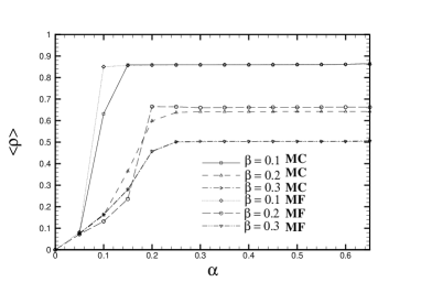
Figure 5: Disorder-averaged densities vs $\alpha$ for various output rates $\beta$. System size is 200 and averaging has been executed over 1000 disordered samples.

Similar to fig. (4), the density value in the saturation regime is roughly 0.5 which is the same as the normal ASEP density value in the MC phase. However, $\langle\rho\rangle$ differs from $1-\beta$ in the LD phase. We note that both high to low and low to high phase transitions which are first order in the normal ASEP are replaced with a smoother behaviour in the presence of disorder. We have extensively performed Monte Carlo simulations for all ranges of $\alpha$ and $\beta$. The simulation results confirm the existence of three phases of LD, HD and maximal current. Furthermore, our simulations show the growth of the maximal-current region and shortening of the sizes of the LD and HD phases. These findings are in agreement with the mean-field based conclusions of Harris and Stinchcombe stinchcombe . If one changes the parameters of the binary distribution function, the overall picture remains qualitatively the same as in the above diagrams. Nevertheless, the quantitative values of both $\langle J\rangle$ and $\langle\rho\rangle$ in the phases depend on the parameters of the distribution functions. More concisely, currents and densities are functional of $f(p)$. In the following figure, we exhibit the phase diagram of disordered ASEP for some binary distribution functions.

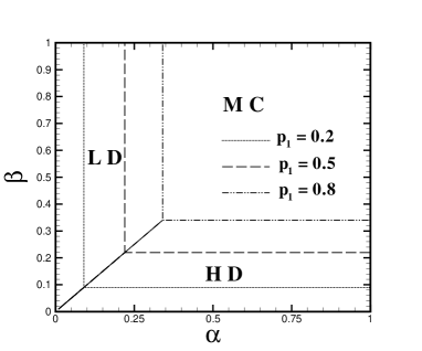
Figure 6: Phase diagram of the disordered ASEP for some binary distributions. The distribution parameters are specified in the figure. All the distributions have $f=0.5$ and $\langle p\rangle=1$ but the variances are different.

We note that the size of the MC phase is an increasing function of the variance of the distribution function. The reason is that currents and densities are dominated by the number of defective sites. If the variance of the distribution is large, then the probability of finding sites with notably small hopping rates is considerable and therefore $\langle J\rangle$ and $\langle\rho\rangle$ are highly affected. The enlargement of the MC phase has been reported for ASEP with a single defect in the bulk kolomeisky1 . We recall from normal ASEP that the critical values of the input and output rates are $\alpha_{c}=\beta_{c}=\frac{p}{2}$ where $p$ is the hopping rate. In principle, since $\alpha,\beta$ and $p$ are rates, they can vary from zero to infinity. Therefore, it is possible to choose the time unit such that $p$ scales to unity. In the disordered version of the ASEP, one does not have a single hopping rate so it would be better not to restrict ourselves to a particular time unit. For the sake of comparison we write the values of the density and current in the low density, high density and maximal current phases of the normal ASEP:

$$\rho_{LD}=\frac{\alpha}{p},~{}\rho_{HD}=1-\frac{\beta}{p},~{}\rho_{MC}=\frac{1}{2}.$$ (4)

Having in the mind that $J=p\rho(1-\rho)$ we thus obtain:

$$J_{LD}=\alpha(1-\frac{\alpha}{p}).$$ (5)

$$J_{HD}=\beta(1-\frac{\beta}{p}).$$ (6)

$$J_{MC}=\frac{p}{4}.$$ (7)

Since in the binary distribution there are three parameters namely $p_{1},p_{2}$ and $f$, we have studied two distinguished cases. First, we restrict ourselves to the condition $\langle p\rangle=fp_{1}+(1-f)p_{2}=1$. This leaves only two free parameters. In the second case, we impose the condition $p_{2}=1$ while $f$ and $p_{1}$ are free to take arbitrary values in $[0,1]$. In the latter case, the emphasis is on the role of defective sites $(p_{1}<1)$ among normal sites $(p_{2}=1)$ whereas the former case allows having fast hopping sites with rate $p_{2}>1$. Our simulations showed that there is no significant differences between the results of these two cases. Therefore in what follows, we only exhibit the results for the case $p_{2}=1$ i.e., slow defective sites among normal sites. Our first set of graphs (all obtained via Monte Carlo simulations) illustrates the dependence of $\langle J\rangle$ on $f$ for various $p_{1}$ in three sets of input and output rates corresponding to low input-high output, high input-low output and high input-high output.

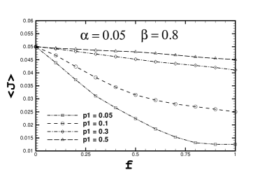
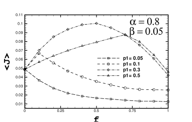
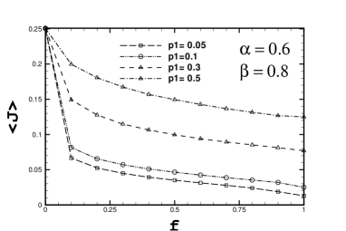
Figure 7: Figures 7-9: $\langle J\rangle$ vs $f$ for various $p_{1}$: $\alpha=0.05,~{}\beta=0.8$ (top), $\alpha=0.8,~{}\beta=0.05$ (middle) and $\alpha=0.6,~{}\beta=0.8$ (bottom). System size is $L=300$.

When $\alpha$ is small and $\beta$ is high (fig.7), the effect of increasing $f$ is to reduce the current. Smaller values of $p_{1}$ exhibit a sharper decrease. This is natural since the bulk density is low and therefore the system current is more sensitive to both the number and the strength of the defects. The dependence of $\langle J\rangle$ on $f$ changes qualitatively when one goes to the situation characterized by high $\alpha$ and low $\beta$ ( fig.8 ). Here we are confronted with unexpected and novel features. For $p_{1}$ less than $0.15$, the current appears as a decreasing function of $f$ while for $p_{1}>0.1$ it increases up to a maximum and then starts diminishing. Accordingly, the optimum value of $f$ at which $\langle J\rangle$ is maximum is no longer $f=0$ but rather a nonzero $f_{max}$. This implies that the effect of disorder is to enhance the current which is a desirable effect. The location of $f_{max}$ shifts towards higher values when one increases $p_{1}$. For large $p_{1}$, $\langle J\rangle$ shows an increasing behaviour with a small slope. The slope tends to zero when $p_{1}\rightarrow 1$. For relatively high values of $\alpha$ and $\beta$ (fig. 9), one still observes that the dependence of current versus $f$ shows a decreasing character. In this case, the disorder has the expected behaviour i.e.; the higher the number of the impurities, the larger the decrease of $\langle J\rangle$. However, the interesting point is the abrupt change in the behaviour of the current reduction. For each $p_{1}$, the current shows a rapid reduction up to a certain $f$ and then decreases very smoothly in a nonlinear fashion. This marks the fact that impurities affect the system beyond a certain relative frequency. These results are in agreement with lakatos2 . To gain a deeper insight, it would be instructive to look at the behaviour of $\langle\rho\rangle$ vs $f$. In low input and high output rates (fig.10), one observes that for low $p_{1}$ the bulk density rises up to a maximum and then decreases even below the value of normal ASEP. One might naively think that increasing the density of defective sites leads to an enhancement of the bulk density due to the formation of high density regions behind them. However, the point is that if the density of defective sites reaches a certain value, the probability of finding defective sites in the vicinity of the first site of the chain increases too.

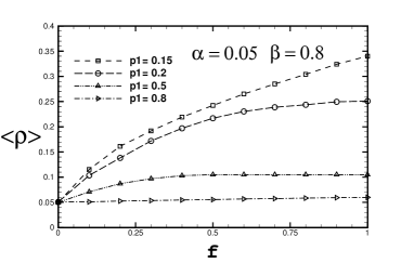
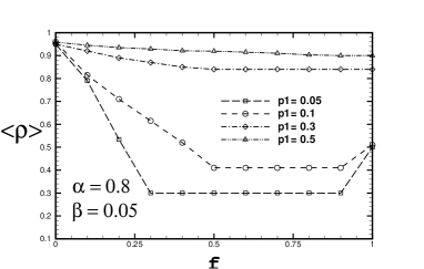
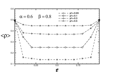
Figure 8: Figures  10-12: Bulk density dependence on $f$ for various values of $p_{1}$: low density phase $\alpha=0.05,\beta=0.8$ (top), high density phase $\alpha=0.8,\beta=0.05$ (middle) and maximal current phase $\alpha=0.6,\beta=0.8$ (bottom). System size is $L=300$.

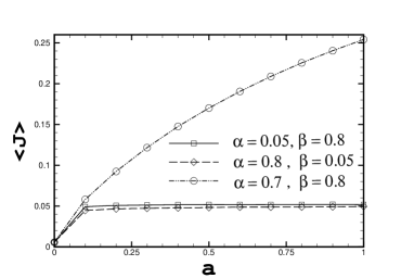
Figure 11: Figure 19 : Average current $\langle J\rangle$ versus $a$ for low $\alpha$ high $\beta$, high $\alpha$ low $\beta$ and high $\alpha$ high $\beta$. $L=200$.

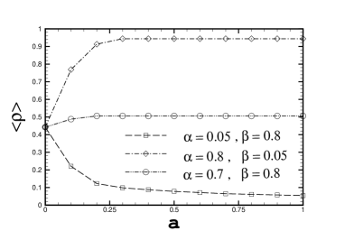
Figure 12: Figure 20 : Average density versus $a$ for low $\alpha$ high $\beta$, high $\alpha$ low $\beta$ and high $\alpha$ high $\beta$. $L=200$.

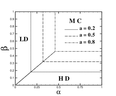
Figure 13: Figure 21 : Phase diagram of the disordered ASEP for a uniform distribution of hopping rates. The distribution characteristics are specified in the figures. All distributions have unit mean but the variances are different.

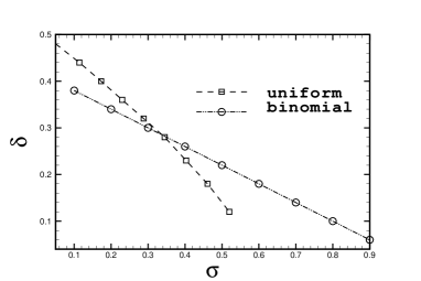
Figure 14: Figure 22 : Size of the low and the high density phases versus the variance for uniform and binary distribution functions ($a=p_{1}$, $f=0.5$ and $\langle p\rangle=1$). $L=200$.

This in turn gives rise to a blocking of the current of particles in the chain bulk. As a result, a large portion of the bulk remains almost in a LD regime which leads to a decreasing in the bulk density throughout the chain. This scenario remains valid for small $p_{1}$. For larger $p_{1}$, one observes the expected increase of the bulk density upon increasing the density of defective sites $f$. The reason is that once the defect strength is reduced below a threshold, the formation of high density regions behind these weak sites will be suppressed and therefore the particles can more easily flow throughout the bulk. As a result of this flow, enough particles can be found in the bulk. This increases the number of local high regions behind defects which in turn give rises to the enhancement of $\langle\rho\rangle$. In the high $\alpha$-low $\beta$ regime (fig. 11) and for $p_{1}<0.2$ the dependence of the bulk density on $f$ is sharply decreasing up to a certain $f$ . Afterwards, $\langle\rho\rangle$ becomes independent of $f$ and a lengthy plateau region forms. At $f=0.9$, $\langle\rho\rangle$ shows a rather linear increase to its asymptotic value $0.5$ in the MC phase. We note that when $f=1$, all the sites are defective. For instance, in the case $p_{1}=0.1$, the critical input and output rates are $\alpha_{c}=\beta_{c}=\frac{p_{1}}{2}=0.05$. In this case $\alpha=0.8,\beta=0.05$ lie in the MC phase and hence $\langle\rho\rangle$ approaches $0.5$ in the limit $f\rightarrow 1$. The reason is that when the input is high and the output is low, impurities give rise to phase segregation behind them barma2 ; kolomeisky1 . The formation of macroscopic low density regions in front of them leads to a sharp reduction of $\langle\rho\rangle$. For $p_{1}>0.2$ the decrease of $\langle\rho\rangle$ becomes much more smooth. The reason is that weaker defects are unable to produce low enough density regions. The other interesting point is that when the input rate is high, increasing the number of defects will prevent a high inflow of particles, which is due to the largeness of $\alpha$ and regulates the flow along the bulk. The overall effect is to reduce $\langle\rho\rangle$ from high $\alpha$ to much lower values. As we had already seen in the current diagrams, in some values of $p_{1}$, this diminishing in the bulk density is accompanied by the current increment as exhibited in fig. (8). Now let us discuss the regime where $\alpha$ and $\beta$ are both greater than $0.5$ (fig. 12). For weak defect strength, the density is almost independent of $f$. For $p_{1}$ less than 0.5, $\langle\rho\rangle$ shows a smoothly decreasing dependence on $f$ until it becomes independent of $f$ and correspondingly a plateau region forms. The length of the plateau is relatively large and becomes larger for smaller values of $p_{1}$. Increasing $f$ beyond the plateau value, one again encounters an increasing behaviour of $\langle\rho\rangle$ until it reaches the normal ASEP value $\langle\rho\rangle=0.5$ in the limit $f=1$ in which all sites have become defective. In order to shed more light on our understanding, we now study the effect of varying the disorder strength $p_{1}$ for fixed values of $f$. Analogous to the previous studies, we first consider the current which is shown in figures (13-15).

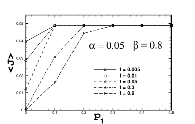
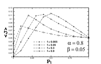
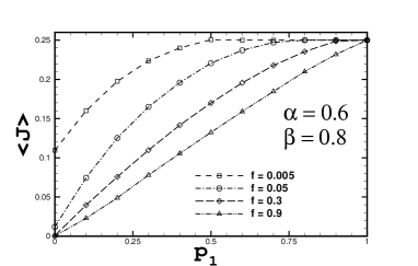
Figure 9: Figures  13-15: Current dependence on $p_{1}$ for various values of $f$: low density phase $\alpha=0.05,\beta=0.8$ (top), high density phase $\alpha=0.8,\beta=0.05$ (middle) and maximal current phase $\alpha 0.6,\beta=0.8$ (bottom). System size is $L=300$.

When $\alpha$ is small and $\beta$ large, the effect of increasing $p_{1}$ is to increase the current to its normal value $\alpha(1-\alpha)$. For each $f$, $\langle J\rangle$ increases with $p_{1}$ up to a certain value and then gets saturated. This implies that below a certain strength, the defect strength is incapable of affecting the current. This picture changes dramatically when large $\alpha$ and small $\beta$ are taken into account. In this case, $\langle J\rangle$ increases with $p_{1}$ up to an $f$-dependent value and then starts decreasing. The maximum current sustained by the system is considerable. While in the case $\alpha=0.8$ $\beta=0.05$, the current for the normal ASEP is $\beta(1-\beta)\sim 0.05$; here we observe that disorder can remarkably enhance the current to almost a doubled value around $0.12$.

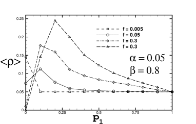
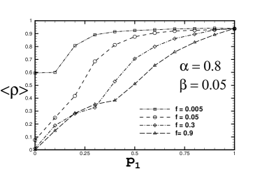
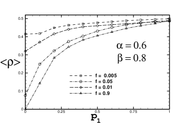
Figure 10: Figures  16-18: $\langle\rho\rangle$ vs $p_{1}$ for various $f$: LD phase $\alpha=0.05,\beta=0.8$ (top), HD phase $\alpha=0.8,\beta=0.05$ (middle) and MC phase $\alpha=0.6,\beta=0.8$ (bottom). System size is $L=300$.

This type of constructive behaviour can be explained on the same grounds as for figure (8). Qualitatively, the impurities do not allow the overflow of particles into the system bulk which otherwise would have led to congestion and current reduction. If $p_{1}$ is small, the strength of defects is sufficient to block the the inflow of particles and reduces the current. If $p_{1}$ is high enough, large inflow $\alpha$ will dominate and $\langle J\rangle$ is reduced. At an intermediate $p_{1}$ we have a maximal current. Analogous to low $\alpha~{}$ high $\beta$, when both $\alpha$ and $\beta$ are large, increasing $p_{1}$ leads to current increments. If the density of defects is high, the current’s increase would be linear in $p_{1}$. For small $f$, the increase in current is rather linear for small $p_{1}$ and afterwards becomes more smooth. To deal in some depth, we next sketch the dependence of $\langle\rho\rangle$ on the defect strength $p_{1}$. For small $\alpha$ and large $\beta$ (see figure (16)), one interestingly observes that if the defect concentration is relatively small i.e., less than 0.02, the effect of decreasing the defect strength (increasing $p_{1}$) is to reduce the density as intuitively expected. Based on our previous arguments, defects are more influential if their concentration is relatively small chou . Therefore, in the small concentration regime, the weakening of the defects leads to a sharp decrease in the density. Beyond a certain $p_{1}$, the further weakening of defects does not affect $\langle\rho\rangle$. For defect concentration $f$ above $0.02$, the behaviour of $\langle\rho\rangle$ undergoes a qualitative change. As observed in figure (16), $\langle\rho\rangle$ increases up to a maximum and then starts diminishing. The maximum value of $\langle\rho\rangle$ depends on $f$ and ranges between $0.11$ and $0.25$. The reason is twofold. First, for small input rate $\alpha$ and intermediate concentration of defects, strong defects are still capable of forming rather large high density regions behind them which results in high $\langle\rho\rangle$. The second reason is due to the blocking of the particles outflow. Although $\beta$ is high, strong enough defects are able to reduce this high outflow rate and effectively reduce it. Consequently, the bulk density rises up throughout the bulk. Below a certain strength, the defective sites, although their numbers are not so small, are not only incapable of forming high density regions behind them but also incapable of effectively reducing the output rate. Therefore, $\langle\rho\rangle$ becomes decreasing. We now consider the case where $\alpha$ is large but $\beta$ is small (see fig. 17). Here the overall effect of decreasing the defect strength is enhancement of $\langle\rho\rangle$. When the defect strength is reduced, the particles can more easily enter the chain and this leads to an increase in the bulk density. In the limit of weak strength $p_{1}\rightarrow 1$, we recover the normal value $\rho=1-\beta$. When both $\alpha$, and $\beta$ are large corresponding to the MC phase in the normal ASEP, we still observe that the effect of a reduction of the defect strength is to enhance the density. Defects can drastically reduce the density if their concentration and their strength are both large. Otherwise, their influence is a slight reduction of the density. We note the type of density increment is rather similar in figures (17) and (18).

IV Uniform distribution function

So far our investigation has been restricted to the case where the disorder strength was limited to only two values. In order to obtain a complimentary insight into the nature of disorder effect, it would be noteworthy to consider the case where the defect’s strength can be chosen from a continuous interval. For this purpose, we consider the uniform distribution function for the strength of defect. Here one has two parameters namely $a$ and $b$ which are the first and last points of the distribution interval. Like the binary distribution, one can introduce two classes. In the first class, $\langle p\rangle=\frac{a+b}{2}=1$ which corresponds to the case having fast hopping sites greater than unity. In the second class, $b=1$ while $a~{}(a<1)$ determines the lower limit of the defect’s value. Note that in the second class $\langle p\rangle=\frac{1+a}{2}<1$. We now exhibit the results for the latter case i.e., $b=1$. The following diagram depicts the dependence of $\langle J\rangle$ on the lower end of the interval $a$. All diagrams which are shown next have been obtained by Monte Carlo simulations. The number of disordered samples over which the averaging have been performed is 1000, and the system size is 200.

According to figure (19), in low $\alpha$-high $\beta$ and high $\alpha$-low $\beta$ regimes, beyond $a=0.1$, the impurities do not affect the current and the system can maintain the normal ASEP values $\alpha(1-\alpha)$ and $\beta(1-\beta)$ respectively. In contrast, for both $\alpha$ and $\beta$ larger than $0.5$, $\langle J\rangle$ is a smooth increasing function of $a$. The current reaches its normal ASEP value $0.25$ in the limit $a\rightarrow 1$. The behaviour of the average bulk density $\langle\rho\rangle$ on $a$ is shown in figure (20).

Contrary to the current diagrams, here the density approaches the normal ASEP value which depends on $\alpha$ and $\beta$. The high $\alpha$-high $\beta$ regime has the weakest dependence on $a$ and beyond $a=0.1$, $\langle\rho\rangle$ will be independent of $a$. Figure (21) depicts the phase diagram in the case where the average rate of hopping is unity: $\langle p\rangle=\frac{a+b}{2}=1$ for various values of $a$. Analogous to the binary distribution, the overall effect of disorder is to enlarge the size of the MC phase and shrinkage of low and high density phases, respectively.

Figure (22), exhibits the size dependence of the LD (HD) phase $\delta$ in terms of the variance of the distribution functions for both uniform and binary distribution functions. The mean of the distribution functions is set to unity.

For the uniform distribution, the size increment of the MC phase shows a more rapid dependence on the variance of the distribution function in comparison to the binary distribution. The reason is due to the fact that in the uniform distribution, the frequency of small-hopping sites close to the lower limit of the distribution interval is more than those in the binary distribution.

V Summary and Concluding Remarks

Let us now summarize what has been explored in this paper. We have investigated the statistical characteristics of the asymmetric simple exclusion process in the presence of spatially uncorrelated quenched disorder in the hopping rates via extensive simulation and numerics. Our findings cover two different distributions of hopping rates: binary and uniform. The conventional three-phase structure of the normal ASEP remains unchanged. Generically, the disorder affects the phase diagram by enlarging the maximal current phase, which in turn leads to squeezing the low and high density phases. This is accompanied by an overall decrease (increase) in the currents (densities). We have managed to numerically solve the mean-field equations. Monte Carlo simulations are in support of the mean field solutions. In brief, the current exhibits a diminishing behaviour in terms of the defect’s concentration in the chain when the input rate is small and the output rate is high. Analogously, it decreases when both the input and output rates are relatively high. Unexpectedly, in the case when the input rate is large and the output rate is small, the current shows an increasing dependence versus the defect’s concentration. This demonstrates the nontrivial interplay of spatial sitewise disorder with the drive. We have also examined the properties of the ASEP under uniformly distributed spatial disorder. Although the phase structure is similar to that of with a binary distribution, we have identified distinctive features between them. Our study has been limited to disorder distribution functions with finite second moments. We expect to observe substantial different types of behaviours for those distributions having a long tail. Work along this line is in progress.

VI acknowledgement

We wish to acknowledge the Institute of Advanced Studies in Basic Sciences (IASBS) for proving us with the computational facilities where the final stages of this work were carried out. Fruitful discussion with Mustansir Barma is appreciated.

References

- [1] M. Sahimi, Rev. Mod. Phys., 65, 1393, (1993); M. Sahimi, Phys. Rep., 306, 295, 1998.
- [2] A. Bunde and S. Havlin (Eds.) in Fractals and disordered systems, 2nd ed., Springer, Berlin, 1996.
- [3] B. D. Hughes in Random walks and random environments, Oxford University Press, Oxford, England, 1995.
- [4] T. Liggett in Interacting Particle Systems: Contact, Voter and Exclusion Processes, Springer, Berlin, 1999.
- [5] B. Schmittmann and R.K.P. Zia in: Phase transitions and Crtitical Phenomena, vol 17, ed. C. Domb and L. Lebowitz (London: Academic) 1995.
- [6] G. Schütz in: Phase transitions and Crtitical Phenomena, vol 19, ed. C. Domb and L. Lebowitz, Academic Press, 2001.
- [7] D. Chowdhury, L. Santen and A. Schadschneider, Physics Reports, 329, 199, 2000.
- [8] H. Hinrischsen, Adv. Phys., 49, 815, 2000.
- [9] J.T. MacDonald, J.H. Gibbs and A.C. Pipkin Biopolymers, 6, 1, 1968; J.T. MacDonald and J.H. Gibbs Biopolymers, 7, 707, 1969.
- [10] B. Derrida, M.R. Evans, V. Hakim and V. Pasquir J. Phys. A, 26, 1493, 1993.
- [11] G. Schütz and E. Domany J. Stat. Phys. , 72, 277, 1993.
- [12] B. Derrida Physics Report, 301, 65, 1998.
- [13] S. Janowsky and J.L. Lebowitz Phys. Rev. A, 45, 618, 1992.
- [14] S. Janowsky and J.L. Lebowitz J. Stat. Phys., 77, 35, 1994.
- [15] M. R. Evans, J. Phys. A: Math,Gen., 30, 5669, 1997.
- [16] G. Tripathy and M. Barma, Phys. Rev. Lett., 78, 3039, 1997.
- [17] G. Tripathy and M. Barma, Phys. Rev. E, 58, 1911, 1998.
- [18] A. B. Kolomeisky, J. Phys. A: Math, Gen., 31, 1153, 1998.
- [19] M. Bengrine, A. Benyoussef, H. Ez-Zahraouy, J. Krug, M. Loulidi and F. Mhirech J. Phys. A: Math, Gen., 32, 2527, 1999.
- [20] K. M. Kolwanker and A. Punnoose, Phys. Rev. E, 61, 2453, 2000.
- [21] C. Enaud and B. Derrida, Europhys. Lett., 66, 83, 2004.
- [22] R. J. Harris and R. B. Stinchcombe, Phys. Rev. E, 70, 016108, 2004.
- [23] T. Chou and G. Lakatos, Phys. Rev. Lett., 93, 198101, 2004.
- [24] L. B. Shaw, A. B. Kolomeisky and K. H. Lee J. Phys. A: Math, Gen., 37, 2105, 2004.
- [25] L. B. Shaw, J.P. Sethna and K. H. Lee Phys. Rev. E, 70, 021901, 2004.
- [26] G. Lakatos, T. Chou and A.B. Kolomeisky, Phys. Rev. E, 71, 011103, 2005.
- [27] , R. Juhasz, L. Santen and F. Iglói, Phys. Rev. Lett., 94, 010601, 2005.
- [28] G. Lakatos, J. O, Brien and T. Chou J. Phys. A, 39, 22533, 2006.
- [29] P.Pierobon, M. Mobilia, R. Kouyos and E. Frey, Phys. Rev. E, 74, 031906, 2006.
- [30] M. Barma, Physica A, 372, 22, 2006.