Currents in a Tokamak

Abstract

A self-consistent analysis of the currents in a tokamak yields the result that the parallel neutralizing current is given simply by the sum of currents commonly called the bootstrap current and the Pfirsch-Schlüter current. An expression is given relating the parallel and perpendicular pressure gradient induced species flow velocities to the total current.

I Introduction

With a self-consistent analysis of the equilibrium currents in a tokamak, one finds that the parallel neutralizing current is given simply by the sum of what are commonly called the bootstrap current and the Pfirsch-Schlüter current. As WoodsWoods (2006) correctly points out, the standard expression for the bootstrap current densityKessel (1994); Wang (1998); Houlberg et al. (1997), $\mathbf{J}_{BS}\simeq(-f_{trap}/B_{\theta})(\partial p/\partial r)\;\hat{b}$, has a nonzero divergence, at odds with the usual property of source-less currents, $\nabla\cdot\mathbf{J}=0$. What Woods fails to mention is that the standard expression for the Pfirsch-Schlüter current densityDendy (1993); Dinklage et al. (2005), $\mathbf{J}_{PS}\simeq(-2\varepsilon\cos\theta/B_{\theta}^{0})(\partial p/\partial r)\;\hat{b}$, suffers the same fate. Together, however, they form the parallel neutralizing current density, $\mathbf{J}_{\parallel}$, which is without divergence.

II Derivation

We begin with the usual equations of plasma equilibrium:

$$\nabla p=\mathbf{J}\times\mathbf{B}\;,\;\mu_{0}\mathbf{J}=\nabla\times\mathbf{B}\;,\;\nabla\cdot\mathbf{B}=\nabla\cdot\mathbf{J}=\mathbf{B}\cdot\nabla p=\mathbf{J}\cdot\nabla p=0\;,$$ (1)

where the total pressure is the sum of the species’ pressures, $p=\sum_{s}n_{s}\mathchoice{{\raise 2.0pt\vbox{\hbox{$\textstyle-$}}\kern-4.47227pt}}{{\raise 2.0pt\vbox{\hbox{$\scriptstyle-$}}\kern-3.3445pt}}{{\raise 2.0pt\vbox{\hbox{$\scriptscriptstyle-$}}\kern-2.35281pt}}{{\raise 2.0pt\vbox{\hbox{$\scriptscriptstyle-$}}\kern-1.84724pt}}\!T_{s}=n_{e}\mathchoice{{\raise 2.0pt\vbox{\hbox{$\textstyle-$}}\kern-4.47227pt}}{{\raise 2.0pt\vbox{\hbox{$\scriptstyle-$}}\kern-3.3445pt}}{{\raise 2.0pt\vbox{\hbox{$\scriptscriptstyle-$}}\kern-2.35281pt}}{{\raise 2.0pt\vbox{\hbox{$\scriptscriptstyle-$}}\kern-1.84724pt}}\!T_{e}+(n_{i}+n_{z})\mathchoice{{\raise 2.0pt\vbox{\hbox{$\textstyle-$}}\kern-4.47227pt}}{{\raise 2.0pt\vbox{\hbox{$\scriptstyle-$}}\kern-3.3445pt}}{{\raise 2.0pt\vbox{\hbox{$\scriptscriptstyle-$}}\kern-2.35281pt}}{{\raise 2.0pt\vbox{\hbox{$\scriptscriptstyle-$}}\kern-1.84724pt}}\!T_{i}$, and $\mathbf{J}$ is the total current density. We know that a present-day tokamak has an ohmic current, $\mathbf{J}_{\Omega}$, and that we will be considering discharges with a neutral beam driven current, $\mathbf{J}_{NBI}$. We work in a concentric circular flux-surface geometry $(r,\theta,\phi)$, Figure 1, related to cylindrical coordinates $(R,\phi,Z)$ by $R=R^{0}+r\cos\theta\equiv R^{0}(1+\varepsilon\cos\theta)\;,\;Z=-r\sin\theta\;,\;\phi=\phi$, where $\hat{\phi}$ is taken along the direction of the plasma current. Various quantities also are defined in a coordinate system aligned to the magnetic field, $(x,y,z)=(r,\perp,\parallel)$, Figure 2, where $\hat{z}=\mathbf{B}^{0}/B^{0}\equiv\hat{b}=(0,b_{\theta},b_{\phi})$, and we assume toroidal symmetry, $\partial/\partial\phi\Rightarrow 0$. The magnetic field takes the form $\mathbf{B}=\mathbf{B}^{0}/(1+\varepsilon\cos\theta)=(0,B_{\theta},B_{\phi})$ in this geometry. Some useful operators and identitiesBook (1977) are:

$$\nabla f=\left(\frac{\partial f}{\partial r}\;,\;\frac{1}{r}\frac{\partial f}{\partial\theta}\;,\;0\right)\;,\;\nabla\cdot\mathbf{F}=\frac{1}{rR}\left[\frac{\partial}{\partial r}rRF_{r}+\frac{\partial}{\partial\theta}RF_{\theta}\right]\;,$$ (2)

$$\nabla\times\mathbf{F}=\left(\frac{1}{rR}\frac{\partial}{\partial\theta}RF_{\phi}\;,\;\frac{-1}{R}\frac{\partial}{\partial r}RF_{\phi}\;,\;\frac{1}{r}\left[\frac{\partial}{\partial r}rF_{\theta}-\frac{\partial}{\partial\theta}F_{r}\right]\right)\;,$$ (3)

$$\nabla\times\nabla f=\nabla\cdot\nabla\times\mathbf{F}=0\;,\;\nabla\cdot(\mathbf{A}\times\mathbf{B})=\mathbf{B}\cdot\nabla\times\mathbf{A}-\mathbf{A}\cdot\nabla\times\mathbf{B}\;,\;\mathbf{A}\cdot\mathbf{B}\times\mathbf{C}=\mathbf{C}\cdot\mathbf{A}\times\mathbf{B}\;.$$ (4)

We note that for nonzero $\mathbf{J}\times\mathbf{B}$, $\nabla p=(\partial p/\partial r)\;\hat{r}$. The ohmic and NBI currents are solely in the toroidal direction, $\mathbf{J}_{\Omega}+\mathbf{J}_{NBI}=(J_{\Omega}+J_{NBI})\;\hat{\phi}$, as is the measured total current $\mathbf{J}=J\;\hat{\phi}$, and satisfy $\nabla\cdot(\mathbf{J}_{\Omega}+\mathbf{J}_{NBI})=0$. The sum of the driven and flow currents is $\mathbf{J}=\mathbf{J}_{\Omega}+\mathbf{J}_{NBI}+\mathbf{J}_{\perp}+\mathbf{J}_{\parallel}$, where $\mathbf{J}_{\perp}$ is the diamagnetic current and $\mathbf{J}_{\parallel}$ is the neutralizing current. The divergence of the diamagnetic current is given by

$$\nabla\cdot\mathbf{J}_{\perp}=\nabla\cdot\left(\frac{\mathbf{B}\times\nabla p}{B^{2}}\right)=(1/B^{2})\nabla p\cdot\nabla\times\mathbf{B}+\mathbf{B}\cdot\nabla p\times\nabla 1/B^{2}-\mathbf{B}/B^{2}\cdot\nabla\times\nabla p=0\;,$$ (5)

and we find that $J^{\perp}_{\theta}=p^{\prime}B_{\phi}/B^{2}$ and $J^{\perp}_{\phi}=-p^{\prime}B_{\theta}/B^{2}$, for $p^{\prime}=\partial p/\partial r$. Turning our attention now to the parallel neutralizing current $\mathbf{J}_{\parallel}$, we find that in order to cancel the poloidal current coming from $\mathbf{J}_{\perp}$, we must have $J^{\parallel}_{\theta}=-J^{\perp}_{\theta}=-p^{\prime}B_{\phi}/B^{2}$ . Then, by similar trianglesHeath and Euclid (1956), Figure 3, we have

$$J^{\parallel}_{\phi}=\frac{B_{\phi}}{B_{\theta}}J^{\parallel}_{\theta}=\frac{-p^{\prime}}{B_{\theta}^{0}}\left(\frac{B_{\phi}^{0}}{B^{0}}\right)^{2}(1+\varepsilon\cos\theta)\equiv J^{BS}_{\phi}+J^{PS}_{\phi}\;,$$ (6)

where we identify the first term as the bootstrap current and the second term as the Pfirsch-Schlüter current. That $\nabla\cdot\mathbf{J}_{\parallel}$ equals zero is given by construction upon noticing that the divergence picks up only the poloidal component. So far, no mention has been made of “passing” versus “trapped” particles, but we note that only passing particles may participate in flowing currents,

$$J=f_{pass}\left[\sigma_{\phi}E_{\phi}+\sum_{s}n_{s}e_{s}\left(u^{\perp}_{\phi}+u^{\parallel}_{\phi}\right)_{s}\right]+J_{NBI}\;,$$ (7)

for toroidal conductivity $\sigma_{\phi}=|b_{\phi}\sigma_{\parallel}-b_{\theta}\sigma_{\perp}|$ and pressure gradient induced species flows $\mathbf{u}^{\perp}_{s}$ and $\mathbf{u}^{\parallel}_{s}$. Thus, one may determine the $E_{\phi}$ profile given the total current, pressure, and magnetic field profiles.

III Conclusions

That the bootstrap current and the Pfirsch-Schlüter current may combine to form a valid, source-less current density should not be a surprise, as the calculation by RossRoss (1995) has indicated for some time. The magnitude of the diamagnetic and neutralizing currents’ contribution to the total plasma current increases with the pressure gradient, suggesting that non-inductive current drive may suffice for sufficiently steep plasma pressure profiles.

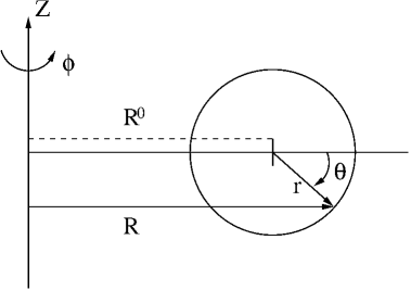
Figure 1: Toroidal Coordinates.

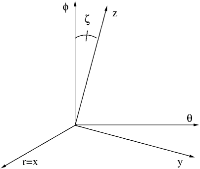
Figure 2: Magnetic Coordinates.

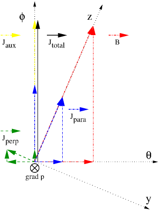
Figure 3: (Color online.) Magnetic Field and the Diamagnetic, Neutralizing, Driven, and Total Currents.

References

- Woods (2006) L. C. Woods, Theory of Tokamak Transport: New Aspects for Nuclear Fusion Reactor Design (Wiley-VCH, 2006).
- Kessel (1994) C. E. Kessel, Nuclear Fusion 34, 1221 (1994), URL http://stacks.iop.org/0029-5515/34/1221.
- Wang (1998) S. Wang, Physics of Plasmas 5, 3319 (1998), URL http://link.aip.org/link/?PHP/5/3319/1.
- Houlberg et al. (1997) W. A. Houlberg, K. C. Shaing, S. P. Hirshman, and M. C. Zarnstorff, Physics of Plasmas 4, 3230 (1997), URL http://link.aip.org/link/?PHP/4/3230/1.
- Dendy (1993) R. Dendy, Plasma Physics: an Introductory Course (Cambridge University Press, Cambridge, England, 1993).
- Dinklage et al. (2005) A. Dinklage, T. Klinger, G. Marx, and L. Schweikhard, eds., Plasma Physics: Confinement, Transport and Collective Effects (Springer, 2005).
- Book (1977) D. L. Book, Tech. Rep. 3332, Naval Research Laboratory (1977).
- Heath and Euclid (1956) T. L. Heath and Euclid, The Thirteen Books of Euclid’s Elements, Books 1 and 2 (Dover Publications, Incorporated, 1956), ISBN 0486600882.
- Ross (1995) D. W. Ross, Tech. Rep. FRCR-473, Fusion Research Center, University of Texas (Austin) (1995).