A thermodynamic model for agglomeration of DNA-looping proteins

Abstract

In this paper, we propose a thermodynamic mechanism for the formation of transcriptional foci via the joint agglomeration of DNA-looping proteins and protein-binding domains on DNA: The competition between the gain in protein-DNA binding free energy and the entropy loss due to DNA looping is argued to result in an effective attraction between loops. A mean-field approximation can be described analytically via a mapping to a restricted random-graph ensemble having local degree constraints and global constraints on the number of connected components. It shows the emergence of protein clusters containing a finite fraction of all looping proteins. If the entropy loss due to a single DNA loop is high enough, this transition is found to be of first order.

I Introduction

Understanding the spatial organization of DNA in the cell / the cellular nucleus and its relation to transcription is one of the big challenges in cell biology Alberts ; Cremer ; Cook ; Kepes ; Segre . In this context, the experimental observation of transcription foci is of great interest: The transcriptional activity is not evenly distributed inside the cell, but it is concentrated in focal points around so-called transcription factories Cook . These factories contain multiple copies of RNA polymerasis, transcription factors and parts of the machinery for post-transcriptional RNA modifications. In order to be transcribed, DNA has to loop back to these transcription factories, it is expected that one factory is surrounded by about 10-20 DNA loops. In this and related phenomenological pictures Kepes ; Segre the formation of transcription factories and DNA looping are considered to be of fundamental importance for the large-scale spatial organization of the transcriptional activity. A sound theoretical understanding grounded on simple physical mechanisms is, however, missing.

The major reason for the increased efficiency of transcription by transcription factories is the following: A locally increased concentration of transcription factors close to target genes enhances recognition of transcription factor binding sites, the volume a transcription factor has to search before finding a target gene is substantially decreased. In bacteria, local concentration effects are partially achieved by the co-localization of genes coding for a transcription factor and their target genes along the one-dimensional chromosome itself mirny . By looping, target genes which are far along the genome can be brought together in cellular / nuclear space. Very recently, it was shown experimantally broek that compact DNA conformations actually enhance target localization compared to stretched conformations. This observation supplies strong support for the importance of coupling transcriptional activity to the spatial DNA organization.

The formation of single DNA loops and its consequences for gene regulation have recently been in the center of interest of many bio-physical research works. These range from precise numerical descriptions of the looping properties of DNA resp. chromatin fibers Bon ; Toan up to the thermodynamic modeling of mechanisms for transcriptional gene-regulation. Both direct looping by bivalent transcription factors (as e.g. the lac repressor) Vilar ; Hwa1 and looping via attractive protein-protein interactions between DNA-bound proteins have been studied Hwa2 ; Saiz . The latter process is important in particular in distal gene regulation in eukaryotic cells Alberts .

In this paper, we assume a more global point of view: May DNA loops and looping proteins agglomerate collectively to give rise to transcriptional foci? What are the thermodynamic ingredients leading to such an agglomeration? In this context, we model the DNA as a string containing many protein binding domains (BD), each one composed of $K$ binding sites (BS). In this work we consider only bivalent DNA-binding proteins which are able to bind simultaneously to two different BDs, introducing thus a DNA loop . Fig. 1 resumes the basic model ingredients. We find that this simple model leads to an effective attraction between DNA loops and thus to the formation of protein agglomerates.

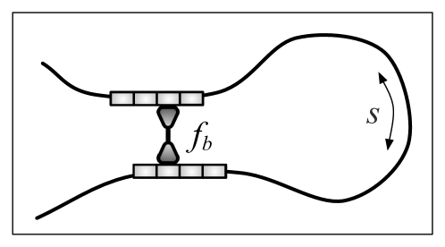
Figure 1: Schematic representation of a single DNA loop with one looping protein: The looping protein binds to single binding sites in two binding domains (each binding domain has $K$ binding sites), leading to a binding free-energy gain of $f_{b}$. A DNA loop leads to an entropy loss $s$.

The role of multiple binding sites for a single loop has already been studied by Vilar et al. Vilar ; Saiz , whereas multiple loops have been considered by Hanke and Metzler Metzler but for BDs with only $K=1$ BS. We will show that only the combination of both is able to introduce the desired emergence of protein agglomerates. This raises an interesting question: given a concentration of looping proteins and an entropy cost of bringing two binding domains in close vicinity, is it possible to get an agglomerate of binding domains? Besides being of interest to transcription factories the question is actually very general and interesting by itself when reformulated differently: If we consider each BD to be a monomer, then the problem is equivalent to understanding the effect of introducing $L$ non nearest neighbour links between $N$ monomers, with global constraints resulting from the entropy loss due to DNA looping, and local constraints due to the structure assumed for the BD.

In the following Sec. II, we first discuss the basic mechanism for protein agglomeration resulting from the combination of these ingredients. Later in this paper, in Sec. III, we introduce a mean-field model which can be mapped to a restricted random-graph ensemble. In Sec. IV, we solve it approximately generalizing a microscopic mean-field approach developed by Engel et al. Engel . In Sec. V, we discuss the results of our mean-field model in the context of factories and compare them with the known results for collapse of randomly linked polymers.

II The basic mechanism

As shown in Fig. 1, there are two competing effects related to DNA looping: First, the binding of a linking protein introduces some free-energy difference $-f_{b}$ (for example in case of lac operon $f_{b}$ is of order 10-15 kcal/mol Vilar2 ). The second contribution comes from the fact that each loop reduces the conformational entropy of the DNA, thus a link leads to a total free-energy difference of $\Delta F=-f_{b}+Ts$, with $T$ being the temperature and $s$ being the entropy loss. In principle $s$ depends on the length of the loop and on the DNA stiffness, cf. Metzler . For this qualitative argument we do not take care of this dependence and use the entropy loss of a typical-length loop.

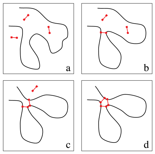
Figure 2: Basic agglomeration mechanism: (a) DNA is represented by a string, binding proteins by linkers. (b) Binding a protein to two BDs leads to a gain of binding free energy, but causes a loss in DNA conformational entropy. (c) The same happens, if a second loop is introduced. (d) Now, if one BD is common to the loops, a next protein may bind to the still unlinked BDs without major entropy losses.

Now, as shown in Fig. 2, we introduce a second loop, and the total free-energy difference to the unlooped configuration becomes $\Delta F=-2f_{b}+2Ts$. There are two possible cases for the relative positions of the two loops: First, the loops are distant, and the binding of another linker protein has to introduce a new loop. Second, loops share one BD. Then also the unconnected BDs of the two loops may be linked, cf. cases (c) and (d) in the figure. In this case, binding free energy is gained, but no new loop is introduced, i.e., no further entropy is lost. We thus have a free energy $\Delta F=-3f_{b}+2Ts$ which is lower than the one achievable by distant loops. This mechanism introduces an effective attraction between binding domains of loops: A cluster of $n$ loops might be connected by $n(n+1)/2$ proteins, so the binding free-energy is growing quadratically with the entropy loss. Note that this picture is based on the simple observation of multiplicity of protein binding sites in a binding domain on DNA.

III A mean-field description via random protein-connection graphs

To gain a first understanding of the action of this effective attraction, we set up a mean-field model. The entropy loss $s$ due to the introduction of a loop is assumed to be independent of the one-dimensional distance between two BDs measured along the DNA chain. Note that this approximation would be exact for monomers in a box.

On this level, BDs can be seen as vertices of a protein-connection graph, and each bound protein between two such vertices forms an edge. We assume $L$ proteins to be bound. The entropy loss due to this linking depends on the component structure of the graph: A connected component (CC) of $n$ vertices contains $n-1$ loops. Denoting the number of CCs of $n$ vertices by $C(n)$, and the total vertex number by $N$, we find that the free-energy difference with respect to the loop-free system is

$$\Delta F = -Lf_{b}+Ts\sum_{n=1}^{N}(n-1)C(n)$$ (1)

$$= -Lf_{b}-TCs+const.$$

with $C=\sum_{n}C(n)$ being the total number of CCs. This free energy has two competing negative contributions. The first term favors large $L$ by binding more proteins, and its ground state would be the fully connected graph which has only one CC. The second contribution in (1) favors many components for positive $s$. Its ground state is thus the empty graph with each of the $N$ isolated vertices as a CC. The global behavior of the model is given by the balance of these two terms, and can be characterized by the partition sum running over all graphs,

$$Z=\sum_{\rm graphs}\exp\{Lf_{b}/T+Cs\}\ .$$ (2)

We note that this partition function describes a modified random-graph ensemble which depends only on the number of links and the number of CCs. In fact, in usual diluted random graphs Erdos each pair of vertices is connected with some probability $0<p<1$, and left unconnected with $1-p$. The probability of a specific graph with $L$ edges is then proportional to $[p/(1-p)]^{L}$, so it is exponential in the number of edges. If, further on, we reweight all graphs by some factor $q^{C}$, we find that the graphs have a probability corresponding to Eq. (2) by identifying $p/(1-p):=e^{f_{b}/T}$ and $q:=e^{s}$. Further more, the sum over all graphs is restricted by the connectivity constraint: At most $K$ proteins can be bound to one BD, for $d$ bound proteins the distinguishable nature of the BS inside the BD results in a combinatorial factor $K!/(K-d)!$. In the next section we give an analytical description of this problem for any $K$.

The main question of this work, i.e. the question if an agglomerate exists or not, translates to the problem of graph percolation: Agglomeration is equivalent to the existence of an extensively large connected component in the graph, i.e. to the existence of a giant component.

IV Analytical description of the graph ensemble

Before coming to the full description of the problem, i.e. to random graphs which have restricted degrees and are reweighted according to their number of CCs, we concentrate a moment on the case $q=1$, i.e. without considering the number of CCs. The basic idea is that the number of CCs can be introduced in a later moment considering large deviations from typical $q=1$-graphs. The approach generalizes the cavity-type calculation of Engel , which is the special case $K=\infty$. We will resort to this limit in order to check correctness of our results.

IV.1 Graphs at $q=1$

First, we describe the graphs without any constraint coming from the number of CCs, i.e. without entropy losses in the DNA-looping model. In this case we have $s=0$, i.e. $q=1$. The graphs have $N$ vertices (or BDs), each of them containing $K$ distinguishable BS (called stubs in the following) which allow vertices to have up to degree $K$. We describe graphs at the level of vertices by their symmetric adjacency matrix $\{J_{ij}\}$ with entries 1 whenever to vertices are connected via any two of their BS, and 0 else. The distinguishable nature of the binding sites is taken into account by a c ombinatorial factor $K!/(K-d)!$ for any vertex of degree $d$. This factor counts the number of non-equivalent way the $d$ edges can be attached to the $K$ BS.

The statistical properties of a graph $G$ with adjacency matrix $\{J_{ij}\}$ can be characterized by its number of links

$$L(G)=\sum_{i<j}J_{ij}$$ (3)

and its degree distribution given via the number $N_{d}$ of vertices of degree $d$,

$$N_{d}(G)=\sum_{i}\delta\left(d,\sum_{j}J_{ij}\right)\ ,\ \ \ d=0,...,K,$$ (4)

with the notation $\delta(\cdot,\cdot)$ for the Kronecker symbol. Obviously these quantities are not independent. We have $\sum_{d}N_{d}=N$ and $\sum_{d}dN_{d}=2L$ since links are counted twice by adding up all degrees. Without reweighting graphs by the number of CCs, the graph ensemble is completely characterized by these quantities. In fact we write

$$P(G|\gamma,K,N) = \frac{1}{Z(\gamma,K,N)}\ \prod_{i<j}\left[\left(1-\frac{\gamma}{K^{2}N}\right)\delta(J_{ij},0)+\frac{\gamma}{K^{2}N}\delta(J_{ij},1)\right]\ \prod_{i=1}^{N}\left[\frac{K!}{(K-\sum_{j}J_{ij})!}\,\Theta(K-\sum_{j}J_{ij})\right]$$ (5)

$$= \frac{1}{Z(\gamma,K,N)}\ \left(\frac{\gamma}{K^{2}N}\right)^{L(G)}\ \left(1-\frac{\gamma}{K^{2}N}\right)^{{N\choose 2}-L(G)}\ \prod_{d=0}^{K}\left[\frac{K!}{(K-d)!}\right]^{N_{d}(G)}\ ,$$

where the last line already takes into account that degrees beyond $K$ are forbidden. In this notation, $\gamma$ acts as a chemical potential for links, and corresponds to the binding free energy in the protein case. Note that the combination $\gamma/(K^{2}N)$ is chosen such that, for $K\to\infty$, we recover normal Erdös-Renyi random graphs with average degree $\gamma$. In this limit, all our results here have to coincide with the ones of Engel .

From this microscopic description by the adjacency matrix of a graph, we can go directly to a coarser description giving the probability of a graph to have some degree distribution $N_{d}=p_{d}N$. We find

$$P(N_{0},...,N_{K}|\gamma,K,N) = \frac{1}{Z(\gamma,K,N)}\ \left(\frac{\gamma}{K^{2}N}\right)^{L}\ \left(1-\frac{\gamma}{K^{2}N}\right)^{{N\choose 2}-L}\ \prod_{d=0}^{K}\left[\frac{K!}{(K-d)!}\right]^{N_{d}}$$ (6)

$$\times\frac{N!}{\prod_{d}N_{d}!}\ (2L-1)!!\ \prod_{d=0}^{K}\left[\frac{1}{d!}\right]^{N_{d}}\ .$$

This equation is obtained by multiplying the probability of a single of these graphs by the number of possible realizations of the degree sequence. The factors are, in the order of appearance, the number of ways to assign degrees to the $N$ vertices, the number of possibilities to wire a set of vertices with given degrees, and a correction of overcounting due to the (at this point) indistinguishable occupied BSs. Note that the factor $(2L-1)!!=(2L)!/2^{L}/L!$ can be easily understood in terms of generating the graph: Once degrees are assigned, each vertex of degree $d$ is assigned $d$ stubs (or half-edges). These are brought into a random permutation, and the first stub becomes connected to the second one, the third to the fourth etc. This procedure overcounts graphs: A factor $2^{-L}$ accounts for possible permutation of the two stubs inside each of the $L$ links, the factor $1/L!$ for permutations of entire links. This procedure does not forbid double links or self-loops, but these are rare and therefore do not influence the global statistical features of the graph ensemble. Using Stirlings formula $\ln N!=N\ln N-N+o(N)$ we can rewrite this as

$$P(N_{0},...,N_{K}|\gamma,K,N) = \frac{1}{Z(\gamma,K,N)}$$ (7)

$$\times\exp\left\{N\left[\ell\ln\left(\frac{\gamma}{K^{2}N}\right)-\frac{\gamma}{2K}+\sum_{d}p_{d}\ln{K\choose d}-\sum_{d}p_{d}\ln p_{d}+\ell\left(\ln[2\ell N]-1\right)\right]+o(N)\right\}$$

$$= \frac{1}{Z(\gamma,K,N)}\ \exp\left\{N\left[-\sum_{d}p_{d}\ln\left({K\choose d}^{-1}p_{d}\right)+\ell\ln\left(\frac{2\gamma\ell}{K}\right)-\ell\right]+o(N)\right\}\ ,$$

where we have used $\ell=L/N=\frac{1}{2}\sum_{d}dp_{d}$. The typical degree distribution, which is realized in this ensemble with probability tending to one in the thermodynamic limit, can be evaluated by the maximum of this expression. Deriving the exponent by $p_{d}$, and using a Lagrange multiplier to ensure normalization of the degree dsitribution, we arrive directly at (overbars always denote typical values)

$$\overline{p}_{d}={K\choose d}\frac{z^{d}}{(1+z)^{K}}\ ,\ \ \ \ z=\sqrt{\frac{2\gamma\overline{\ell}}{K^{2}}}\ .$$ (8)

With the average degree determined from this distribution,

$$\overline{d}=2\overline{\ell}=K\frac{z}{1+z}\ ,$$ (9)

we arrive at two self-consistent equations for $z$ and $\overline{d}$ which are solved by (a second non-physical solution is not shown)

$$z = \frac{1}{2}\left(\sqrt{1+4\frac{\gamma}{K}}-1\right)$$

$$\frac{\overline{d}}{K} = \frac{\sqrt{1+4\frac{\gamma}{K}}-1}{\sqrt{1+4\frac{\gamma}{K}}+1}\ .$$ (10)

Note that, for $K\to\infty$, the degree distribution (8) tends as expected to the Poissonian law $e^{-\gamma}\gamma^{d}/d!$. These results allow us to express also the dominant contribution to the partition function $Z(\gamma,K,N)$ by the exponent in Eq. (7) evaluated at the saddle point:

$$\frac{1}{KN}\ln Z(\gamma,K,N)=-\frac{\overline{d}}{K}\ln\frac{\overline{d}}{K}-\left(1-\frac{\overline{d}}{K}\right)\ln\left(1-\frac{\overline{d}}{K}\right)+\frac{\overline{d}}{2K}\ln\left(\frac{\gamma}{K}\frac{\overline{d}}{K}\right)-\frac{\overline{d}}{2K}+o(1)\ .$$ (11)

IV.2 The case $q\neq 1$

Now we have all results being important for analyzing the full model including entropy losses. In difference to the case discussed so far, the full graph ensemble includes a weight $q^{C(G)}$ depending on the number $C(G)$ of connected components of graph $G$. We therefore consider the modified ensemble

$$P(G|\gamma,q,K,N)=\frac{1}{Z(\gamma,q,K,N)}P(G|\gamma,q,N)q^{C(G)},$$ (12)

where the normalizing partition function is given as

$$Z(\gamma,q,K,N)=\sum_{G}P(G|\gamma,q,N)q^{C(G)}\ .$$ (13)

Note that this partition function fulfills $Z(\gamma,q\!=\!1,K,N)=1$ due to the use of the normalized distribution $P(G|\gamma,q,N)$ in Eq. (12).

Compared to the previous section, this graph ensemble is hard to handle: The distribution depends on the global quantity $C(G)$ which cannot calculated as easily as the degree distribution, which was sufficient to characterize the graph ensemble at $q=1$. To get information, we modify the cavity-type approach of Engel . There, information on the graph ensemble with $C$-dependent weight (but without degree constraint, i.e. the case $q\neq 1$ and $K\to\infty$) was obtained via a simple and intuitive idea: If we add a new vertex to a typical graph of size $N$, and the degree of this vertex is randomly selected according to the typical degree distribution of size-$N$ graphs, the new graph is basically equivalent to a typical graph of size $N+1$. Unfortunately, this argument holds only approximately in our case. The added vertex does not become a typical one of the enlarged graph. However, since it holds for $K\to\infty$ and for $K=1$, so we expect it to be rather precise also for intermediate-large $K$.

Assume therefore that we add a vertex to a graph $G$ of $N$ vertices. The degree $d$ of this vertex is drawn randomly from $\overline{p}_{d}={K\choose d}z^{d}/(1+z)^{K}$ with $z$ given by Eq. (10) (graph ensemble at $q=1$). Now, the number of components changes according to

$$P(C|\gamma,K,N+1)=\sum_{\Delta C}\tilde{D}(\Delta C)P(C+\Delta C|\gamma,K,N)\ .$$ (14)

The kernel $\tilde{D}(\Delta C)$ can be decomposed into various contributions according to the degree $d$ of the new vertex, and the number $d_{0}$ of links this new vertex makes with the giant component of $G$. The change $\Delta C$ of the number of CCs also depends on these two numbers. For positive $d_{0}>0$, we add $d-d_{0}$ small components to the giant one, i.e. we have $\Delta C=d-d_{0}$. For $d_{0}=0$, we unify $d$ small components to a single one, and we have $\Delta C=d-1$. The kernel therefore results in

$$\tilde{D}(\Delta C) = \sum_{K\leq d\leq d_{0}\leq 0}\tilde{D}(\Delta C,d,d_{0})\ ,$$

$$\tilde{D}(\Delta C,d,d_{0}) = \alpha\overline{p}_{d}{d\choose d_{0}}\pi^{d_{0}}(1-\pi)^{d-d_{0}}\delta(\Delta C,d-d_{0}-\delta(d_{0},0))\ ,$$ (15)

with $\pi$ denoting the probability of selecting an end-vertex inside the giant component. Due to the special definition of our ensemble, where we do not select directly vertices but free BS associated to a vertex, the number $\pi$ equals therefore the fraction of all free BS being inside the giant component. It has a simple relation to the fraction $\nu$ of vertices belonging to the giant component:

$$\pi=\frac{K-\overline{d}_{in}}{K-\overline{d}}\nu\ .$$ (16)

Here $\overline{d}_{in}$ denotes the average degree inside the giant component, $\overline{d}$ the one of the full graph.

The reweighting factor $\alpha$ can be calculated exactly in the case $K\to\infty$, cf. Engel . Its precise value is not of interest in our discussion. If we multiply Eq. (14) by $q^{C}$ and sum over $C$, we obtain

$$Z(\gamma,q,K,N+1) = \sum_{\delta C}\tilde{D}(\Delta C)q^{-\delta C}Z(\gamma,q,K,N)$$ (17)

$$= \zeta(\gamma,q,K)\ Z(\gamma,q,K,N)\ .$$

The logarithm of $\zeta(\gamma,q,K)$ can be interpreted as a free-energy shift in the graph ensemble due to adding a new vertex. Using Eq. (15) it can be calculated right away, resulting in

$$\zeta(\gamma,q,K)=\alpha\left[\frac{q+z(1-\overline{\pi})}{q(1+z)}\right]^{K}\left[q-1+\left\{1+\frac{qz\overline{\pi}}{q+z(1-\overline{\pi})}\right\}^{K}\right]\ .$$ (18)

Note that due to the concentration of intensive quantities to their typical values in the summation over all graphs, we have replaced $\pi$ by its saddle-point value $\overline{\pi}$.

The decomposition of $\tilde{D}(\Delta C)$ helps to get more detailled insight into the graph structure. In fact, the quantity

$$\zeta(d,d_{0}|\gamma,q,K) = \sum_{\Delta C}\tilde{D}(\Delta C,d,d_{0})\ q^{-\delta C}$$ (19)

$$= \alpha\overline{p}_{d}{d\choose d_{0}}\overline{\pi}^{d_{0}}(1-\overline{\pi})^{d-d_{0}}q^{-d+d_{0}+\delta(d_{0},0)}$$

describes an effective single-vertex Boltzmann factor, and single-vertex quantities as the probability of belonging to the giant component or the degree distribution can be derived from it.

To start with the giant component size, we remind that for all $d_{0}>0$ the newly added vertex becomes connected to the giant component, and thus is part of it in the $(N+1)$-vertex graph. Therefore the fraction of vertices not belonging to the giant component can be written as

$$1-\overline{\nu} = \frac{1}{\zeta(\gamma,q,K)}\sum_{d=0}^{K}\zeta(d,d_{0}=0|\gamma,q,K)$$ (20)

$$= \frac{q}{q-1+\left\{1+\frac{qz\overline{\pi}}{q+z(1-\overline{\pi})}\right\}^{K}}\ .$$

The degree distribution of the graph results in

$$P(d|\gamma,q,K) = \frac{1}{\zeta(\gamma,q,K)}\sum_{d_{0}=0}^{d}\zeta(d,d_{0}|\gamma,q,K)$$ (21)

$$= {K\choose d}\ \frac{\left[\frac{z(1-\overline{\pi})}{q}\right]^{d}\left[q-1+\left\{1+q\frac{\overline{\pi}}{1-\overline{\pi}}\right\}^{d}\right]}{\left[\frac{q+z(1-\overline{\pi})}{q}\right]^{K}\left[q-1+\left\{1+\frac{qz\overline{\pi}}{q+z(1-\overline{\pi})}\right\}^{K}\right]}\ .$$

For $q\neq 1$, this distribution deviates from a simple binomial distribution. The average vertex degree follows immediately,

$$\frac{\overline{d}}{K} = z\ \frac{(1-\overline{\pi})(q-1)+[1+\overline{\pi}(q-1)]\left\{1+\frac{qz\overline{\pi}}{q+z(1-\overline{\pi})}\right\}^{K-1}}{[q+z(1-\overline{\pi})]\left[q-1+\left\{1+\frac{qz\overline{\pi}}{q+z(1-\overline{\pi})}\right\}^{K}\right]}$$ (22)

$$= \frac{z(1-\overline{\nu})(1-\overline{\pi})}{q[q+z(1-\overline{\pi})]}\left[q-1+\left\{1+\frac{q\overline{\pi}}{1-\overline{\pi}}\right\}\left\{1+\frac{q\overline{\nu}}{1-\overline{\nu}}\right\}^{\frac{K-1}{K}}\right]\ ,$$

where we have used Eq. (20) to simplify the expression in the second line. The degree distribution inside (resp. outside) the giant component can be obtained by restricting sums to $d_{0}>0$ (resp. $d_{0}=0$),

$$P_{\rm in}(d|\gamma,q,K) = \frac{\sum_{d_{0}=1}^{d}\zeta(d,d_{0}|\gamma,q,K)}{\sum_{d=1}^{\infty}\sum_{d_{0}=1}^{d}\zeta(d,d_{0}|\gamma,q,K)}\ ,$$

$$P_{\rm out}(d|\gamma,q,K) = \frac{\zeta(d,d_{0}=0|\gamma,q,K)}{\sum_{d=0}^{\infty}\zeta(d,d_{0}=0|\gamma,q,K)}\ .$$ (23)

For the outside average degree we obtain the particularily simple result

$$\overline{d}_{\rm out}=K\frac{z(1-\overline{\pi})}{q+z(1-\overline{\pi})}\ .$$ (24)

For the inside average degree, we use the fact that the total average degree is the weighted average of the inside and outside degrees, and we find

$$\overline{d}_{\rm in}=\frac{\overline{d}-\overline{d}_{\rm out}(1-\overline{\nu})}{\overline{\nu}}\ .$$ (25)

IV.3 The phase diagram

We have now enough equations to determine self-consistently the phase diagram. Putting together Eqs. (16,20,22,24) and (25), and eliminating directly the expression for $\overline{d}_{\rm in}$, we find a closed set of three equations

$$\overline{\pi} = \frac{1}{K-2\overline{\ell}}\left[K\overline{\nu}-2\overline{\ell}+K\frac{z(1-\overline{\pi})(1-\overline{\nu})}{q+z(1-\overline{\pi})}\right]$$

$$\overline{\ell} = \frac{K}{2}\ \frac{z(1-\overline{\nu})(1-\overline{\pi})}{q[q+z(1-\overline{\pi})]}\left[q-1+\left\{1+\frac{q\overline{\pi}}{1-\overline{\pi}}\right\}\left\{1+\frac{q\overline{\nu}}{1-\overline{\nu}}\right\}^{\frac{K-1}{K}}\right]$$ (26)

$$\overline{\nu} = 1-\frac{q}{q-1+\left\{1+\frac{qz\overline{\pi}}{q+z(1-\overline{\pi})}\right\}^{K}}\ .$$

We had introduced the model in function of the parameter $\gamma$ which can be understood as a chemical potential coupled to the number of edges in the graph. Since this parameter has no very obvious interpretation due to its interaction with the degree-constraints, we prefer to use its conjugate quantity, the link density $\overline{\ell}$ as a control parameter. In this sense, for given $K$, the phase diagram is spanned by $q$ and $\overline{\ell}$, and Eqs. (IV.3) allow to determine the unknown quantities $\overline{\nu},\overline{\pi}$ and $\gamma$.

Eqs. (IV.3) always have the solution $\{\overline{\nu},\overline{\pi},\gamma\}=\{0,0,2\overline{\ell}qK/(K-2\overline{\ell})\}$. It corresponds to a phase without any extensive CC, i.e. to a non-agglomerated phase. For large enough $\overline{\ell}$ and $q=e^{s}$, also other solutions exist. To see this, we expand Eqs. (IV.3) up to second order in $\overline{\nu}$ and $\overline{\pi}$, and find in particular

$$\overline{\pi}=-\frac{K[2\overline{\ell}(K-1)-K]}{2\overline{\ell}^{2}(K-1)[2+K(q-2)]}$$ (27)

which implies a continuous transition to a non-trivial solution at

$$\overline{\ell}_{c}=\frac{K}{2(K-1)},~{}~{}\forall~{}q<q_{c}=2-\frac{2}{K}$$ (28)

Note that, for $K\to\infty$ and $q=1$, this result reproduces the known percolation result in Erdös-Rényi random graphs. For $q<q_{c}$, for all $K$, Eq. (27) implies that $\overline{\pi}\sim(\overline{\ell}-\overline{\ell}_{c})$ near the transition point. At $q=q_{c}$, we can expand Eqs. (IV.3) up to third order in $\overline{\nu}$ and $\overline{\pi}$. We find that there is a percolating point at same value of $\overline{\ell}_{c}$ as for $q<q_{c}$, but with $\overline{\pi}\sim(\overline{\ell}-\overline{\ell}_{c})^{1/2}$. Note that this transition exists for all $K>2$, at $K=2$ itself the transition point would be $\overline{\ell}_{c}=1$ which equals the highest possible degree in this graph (due to $2\overline{\ell}\leq K$).

For $q>q_{c}$, Eq. (27) does not make sense. We find a discontinuous transition at smaller $\overline{\ell}_{c}(q,K)$ which has to be determined from Eqs. (IV.3) via the spinodal point; the transition point can be obtained with good precision using symbolic manipulation software like Mathematica Mathematica . In this case, the largest component jumps from a non-extensive size to a finite fraction of the full system. In Fig. 3, the phase diagram for various values of $K$ is given. It is found to be qualitatively similar for all $K\geq 3$, but agglomeration is favored for higher-order BDs at same number of links. In the inset of the figure we show also the discontinuous nature of the transition: At given number of links the parameter $q$ is changed, and the size of the largest CC is recorded. We find an excellent agreement between MC simulations of random graphs using Metropolis type rewiring steps, and the analytical results obtained from Eqs. (IV.3). This illustrates the quality of approximation done in the analytical approach under vertex addition.

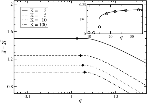
Figure 3: Phase diagram for protein agglomeration in mean-field description for $K=3,5,10,100$: Below the line, no extensive CC exists. Above, a finite fraction of all links and vertices is collected in the largest CC. The transition is continuous on the left, discontinuous on the right side of the diamonds. Inset: Fraction of vertices collected in the largest component as function of $q=e^{s}$, for $\overline{\ell}=0.2$ and $K=20$. The full line is the analytical result of Eqs. (IV.3), the symbols show results of MC simulations for $N=5000$, each symbol is an average over 900 independent equilibrium configurations.

It is very interesting that the phase transition appears at smaller $\overline{\ell}$ for higher entropy losses $s=\ln q$. The reason is that an increased $s$ leads to a compaction of the giant component, where links can be added without loosing further CCs. Therefore, even if the transition appears at lower global average degree, the average degree inside the largest CC always exceeds two. Again, this fact illustrates why $K>2$ is essential for agglomeration.

The left panel of Fig. 4 shows the plot of the average degrees inside and outside the giant component for $q=10$, and for different values of $K$. For all $K\geq 3$, both $\overline{d}_{\rm in}$ and $\overline{d}_{\rm out}$ show clearly a discontinous jump at a critical $K$-dependent value of $\overline{\ell}$. On one hand, $\overline{d}_{\rm in}$ always jumps to a value slightly above two being necessary for the largest component to be connected. The degree outsite the giant component, on the other hand, jumps to values which become smaller and smaller with increasing $K$. In the right panel of Fig. 4, we also show the fraction of vertices resp. edges being in the giant component. For higher $K$ values, the fraction of vertices becomes smaller at the transition point, whereas the fraction of links becomes larger. This illustrates that, for larger $K$, the agglomerate at the threshold becomes smaller but more dense.

Similarly, it is illustrative to look at the properties of the giant component for various values of of $q$. Fig. 5 shows the plots for $K=5$ at $q=5,10$ and $20$. We see that, as $q$ increases, the fraction of vertices inside the giant component goes down (right panel), but the fraction of edges goes up, implying that the agglomerate becomes more and more compact with increasing $q$. Also the difference between the indegree and outdegree goes up as $q$ increases (left panel).

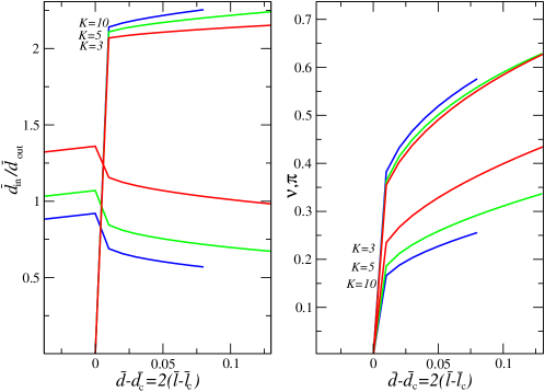
Figure 4: Left panel: Average degrees $\overline{d}_{\rm in}$ inside (upper curves) and $\overline{d}_{\rm out}$ outside the giant component (lower curves), as a function of the total link density $\overline{\ell}$, for values $K=3,5,10$ and fixed $q=10$. Right panel: Fraction $\overline{\nu}$ of vertices (lower curves) and fraction of links (upper curve) for the same parameters as in the left panel.

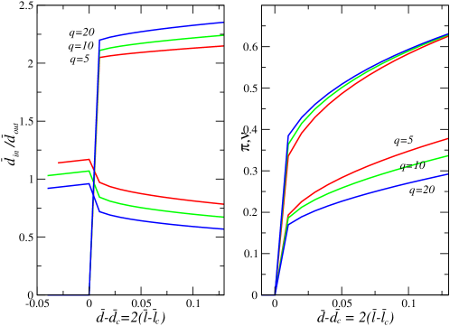
Figure 5: Left panel: Average degrees $\overline{d}_{\rm in}$ inside (upper curves) and $\overline{d}_{\rm out}$ outside the giant component (lower curves), as a function of the shifted link density $\overline{\ell}-\overline{\ell}_{c}$, for fixed $K=5$ and diverse values of $q=5,10,20$. Right panel: Fraction $\overline{\nu}$ of vertices (lower curves) and fraction of links (upper curve) for the same parameters as in the left panel.

V Discussion

The aim of the present paper is to present a minimal model which, on the basis of a thermodynamic approach to DNA-protein interactions, is able to show protein agglomeration. In this sense, it can serve as a minimal model for the mechanism behind the formation of transcription factories, which are observed in transcriptionally active cells. In our paper we show that two ingredients are sufficient: DNA-looping proteins which are able to bind simultaneously to two – also distant – protein binding sites on the DNA, and binding domains on the DNA which contain, on average, more than two binding sites each. In this case, the competition between free-energy gain by protein binding and entropy loss by DNA looping is found to lead to an effective attraction between DNA loops. As a consequence, binding domains and proteins agglomerate collectively.

In its minimal character, the model might miss some important properties of the biological system. As an example, we consider the number of doubly-bound proteins as one important control parameter, whereas the relevant parameter should be the total number of proteins - which would also include free and singly bound molecules. Using biologically reasonable parameters for the binding affinities (ca. 5-15 kcal/mol), we find in simulations that basically none of the proteins stay free and a large majority is doubly bound in the phase-transition region. It would be interesting if we could extend our analytical model accordingly.

Further more, our model did not consider the specificity of interaction between DNA-binding proteins and their binding sites. This specificty may result in the simultaneous agglomeration of various specific transcription factories, which actually is an important ingredient to Cook ; Kepes . Including this possibility into our model would be another interesting generalization, but it would not effect the very basic agglomeration mechanism.

Our model of agglomeration is similar to models of randomly linked polymers studied in the literature. Previous studies mostly considered a Gaussian chain with randomly placed links using variational Bryngelson and numerical methods Kantor . Bryngelson et al Bryngelson in their study based on variational approach and scaling arguments tried to argue that for a Gaussian chain when the links are soft, there is always a transition. They also argued that it is a continuous transition that occurs above a threshold which is a product of the density of links and logarithm of average length of the loop. This result implied that for some arbitrary polymer, it is possible for transition to occur at vanishing density of links ($\sim 1/\ln N$). This result was countered by Kantor et al Kantor . Based on scaling arguments they argued that number of links $M$ necessary for a percolating collapsed phase to exist scale as $N^{\phi}$, with $\phi=1-1/d\nu$, where $\nu$ is the exponent which describes the shape of the polymer (radius of gyration $R_{g}\sim N^{\nu}$). Also, for the probability of looping $p(l)\sim A/l^{\alpha}$, with $1<\alpha<2$, it was shown by Schulman and Newman Schulman that for $M<N/2$ no infinite percolating cluster exists. For $M\geq N/2$, percolation may or may not occur depending on the value of $A$ and $\alpha$.

Our solution correspond to the case where we have ignored length dependence of the entropy cost of the loop ($\alpha=0$) and we find that there would always be a transition from extended phase to collapsed phase, though the nature of transition depends on the entropy cost ($s=-\ln A$) of the loop. Most surprisingly, larger the cost of looping, smaller is the concentration at which the transition happens. Also it is no longer a second order percolation like transition, but a first order transition for low concentration of links.

We did simulations for a Gaussian chain in three dimensions: In our mean-field model we considered entropy losses to be independent of distance between the BDs measured along the DNA. The distance dependence of entropy in vivo is complicated. If we assume that the unlinked DNA behaves on long scales like a Gaussian chain, the entropy loss is monotonously increasing in the the loop length and scales as $q(l)=e^{s(l)}\sim(l/l_{0})^{3/2}$, where $l_{0}$ is the minimum distance between two ends of a loop. If we now look to a connected component of the $n$ vertices $\{i_{1},...i_{n}\}$ with $i_{m}<i_{m+1}$ for all $1\leq m<n$, the entropy loss is given by $s(i_{1},...i_{n})=\sum_{m=1}^{n-1}s(i_{m+1}-i_{m})\,$. In our simulations, we find that there is still a discontinuous transition which depends on the choice of $l_{0}$ (see Fig. 6). Since longer loops are suppressed compared to shorter ones, one could expect CC to be more localized in one-dimensional distance along the DNA. This would correspond to Cook’s picture where DNA loops around a factory form a kind of rosetta, before DNA goes to the next factory. The logarithmic entropy dependence taken into account in our simulations is not sufficient for such a localization.

Based on these simulations, we suggest that even when we take length dependence into account, there is a possibility of first order transition to the agglomerate, at small density of links for high entropy cost. The reason this could be possible would be because of the larger (exponential) contribution of the distribution of links to the entropy in comparision to the lograthimic dependence of entropy on length.

We have ignored the interaction between loops. It is not clear how important that could be. For example, in the case of DNA denaturation Poland , exact results which ignore interaction between loops predict a continuous transition in all dimensions less than four. Whereas using scaling arguments and taking interaction of loop with rest of the chain into account, Kafri et al Kafri showed that the transition becomes first order in $d=2$.

Figure 6: We consider the contribution of entropy loss to the change in free energy for a loop between two BDs to be equal to $s(-\ln l_{0}+\frac{3}{2}\ln l)$. The figure plots the fraction of sites in the giant component for $K\rightarrow\infty$ as a function of $s$ for a chain with $N=5000$ binding domains and $1000$ transcription factors.

The present work can be extended into various directions. First, from biological point of view it would be interesting to go to more realistic modeling schemes (like worm-like chains for the DNA molecule) and to check the proposed picture. Such a simulation would also allow to introduce biologically realistic parameters for protein binding affinities and entropy losses, and to locate such a realistic setting in the simplified mean-field phase diagram. However, current simulations are concentrated to a single loop Bon ; Toan , so this task seems to pose a considerable numerical challenge. It would be interesting to see if self exclusion, depletion effects due to macromolecular crowding or restricted volume would lead to a spatial localization of the agglomerate. A second direction could be the inclusion of diverse looping proteins with specific binding sites on the DNA to see whether equilibrium thermodynamics can drive the creation of transcription factor specific spatial foci. Further, it would be interesting to see perhaps with the help of simulations for Gaussian and self-avoiding chains if one can see a regime of discontinuous transition from extended to collapsed phase.

Acknowledgment — We warmly thank F. Képès and O. Martin for many helpful discussions. We are also thankful to H. Orland for pointing out the reference Bryngelson to us. This work was support by the EC via the STREP GENNETEC (“Genetic networks: emergence and complexity”).

References

- (1) B. Alberts, A. Johnson, J. Lewis, M. Raff, K. Roberts, and P. Walter, Molecular Biology of the Cell (Garland, New York 2002).
- (2) T. Cremer, C. Cremer, Nat. Rev. Gen. 2, 292 (2001); C. Lanctot, T. Cheutin, M. Cremer, G. Cavalli, T. Cremer, Nat. Rev. Gen. 8, 104 (2007).
- (3) P.R. Cook, Science 284, 1790 (1999); P.R. Cook, Nat. Gen. 32, 347 (2002).
- (4) F. Képès, J. Mol. Biol. 329, 859 (2003); F. Képès, C. Vaillant, Complexus 1,171 (2003).
- (5) M.A. Wright, P. Kharchenko, G.M. Church, and D. Segre, Proc. Nat. Acad. Sci. 104, 10559 (2007).
- (6) G. Kolesov, Z. Wunderlich , O.N. Laikova, M.S. Gelfand, and L.A. Mirny, Proc. Nat. Acad. Sci. 104, 13948 (2007).
- (7) B. van den Broek, M.A. Lomholta, S.M.J. Kalisch, R. Metzler, and G.J.L. Wuite, Proc. Nat. Acad. Sci. 105, 15738 (2008).
- (8) M. Bon, D. Marenduzzo, P.R. Cook, Structure 14, 197 (2006).
- (9) N.M. Toan, D. Marenduzzo, P.R. Cook, C. Micheletti, Phys. Rev. Lett. 97, 178302 (2006).
- (10) J.M.G. Vilar and S. Leibler, J. Mol. Biol. 331, 981 (2003).
- (11) L. Bintu, N.E. Buchler, H.G. Garcia, U. Gerland, T. Hwa, J. Kondev, T. Kuhlman, and R. Phillips, Current Opinion in Genetics & Development 15, 125 (2005).
- (12) N.E. Buchler, U. Gerland, and T. Hwa, Proc. Nat. Acad. Sci. 100, 5136 (2003).
- (13) J.M.G Vilar and L. Saiz, Phys. Rev. Lett. 96 238103 (2006).
- (14) A. Hanke, R. Metzler, Biophys. J. 85, 167 (2003).
- (15) A. Engel, R. Monasson, A.K. Hartmann, J. Stat. Phys. 117, 387 (2004).
- (16) J.M.G Vilar and L. Saiz, Current Op. in Gen. and Dev., 15, 136(2005).
- (17) P. Erdös, A. Rényi, Publicationes Mathematicae 6, 290 (1959).
- (18) Mathematica 2005 Wolfram Reseach, htt://www.wolfram.com
- (19) Bryngelson J D and Thirumalai D, Internal Constraints Induce Localization in an Isolated Polymer Molecule, 1996, PRL 76 542.
- (20) Kantor Y and Kardar M, Conformations of randomly linked polymers, 1996, PRE 54 5263.
- (21) Schulman L.S,Long range percolation in one dimension, 1983, J. Phys. A 16, L 639; C.M.Newman and Schulman L.S. …. 1986, Commun. Math. Phys. 104 547.
- (22) Poland D and Scheraga H A, 1966 J. Chem. Phys. 45 1456; Fisher M. E. 1966 J. Chem. Phys. 45 1469.
- (23) Kafri Y, Mukamel D and Peliti L, Why is the DNA Denaturation Transition First Order?,