Decoherence versus disentanglement for two qubits in a squeezed bath.

Abstract

We study the relation between the sudden death and revival of the entanglement of two qubits in a common squeezed reservoir, and the normal decoherence, by getting closer to the Decoherence Free Subspace and calculating the effect on the death and revival times.

I
Introduction

In one-party quantum systems, coherence is destroyed by the action of the environment, a phenomena that is local and occurs asymptotically in time.

On the other hand, there could be multiparty systems, with non-local quantum correlations, often referred to as quantum entanglement. The non-locality and coherence of the quantum entangled states makes them very important in applications such as quantum teleportation t , quantum cryptography cr , dense coding c , etc.

If the environment would act on the various parties the same way it acts on single systems, one would expect that a measure of entanglement, say the concurrence, would also decay exponentially in time.

However, this is not always the case. Recently Yu and Eberly e1 ; e2 ; e3 showed that under certain conditions, the dynamics could be completely different and the quantum entanglement may vanish in a finite time. They called this effect ”entanglement sudden death”. This effect has also been observed experimentally d .

A popular measure of entanglement is the concurrence WO . For pure states is defined as:

$$C(\Psi)=|\langle\Psi|\widetilde{\Psi}\rangle|,$$ (1)

where:

$$|\widetilde{\Psi}\rangle_{12}=(\sigma_{y}^{1}\otimes\sigma_{y}^{2})\otimes|\Psi\rangle_{12},\quad\text{for two qubits.}$$ (2)

For a mixed state, the concurrence is defined as:

$$C(\rho)=max\{0,\sqrt{\lambda_{1}}-\sqrt{\lambda_{2}}-\sqrt{\lambda_{3}}-\sqrt{\lambda_{4}}\},$$ (3)

where the $\sqrt{\lambda_{i}}$ are the eigenvalues($\lambda_{1}$ being the largest one)of a non-Hermitian matrix $\rho\widetilde{\rho}$,  and $\widetilde{\rho}$ is defined as:

$$\widetilde{\rho}=(\sigma_{y}^{1}\otimes\sigma_{y}^{2})\rho^{\ast}(\sigma_{y}^{1}\otimes\sigma_{y}^{2}),$$ (4)

$\rho^{\ast}$ being the complex conjugate of $\rho$.

In this paper we will explore the relation between the sudden death (and revival) of the entanglement between the two two-level atoms in a squeezed bath and the normal decoherence and the decoherence free subspace (DFS), which in this case is a two-dimensional plane.

II The model

In the present work, we consider two two-level atoms that interact with a common squeezed reservoir, and we will focus on the evolution of the entanglement between them, using as a basis, the Decoherence Free Subspace states, as defined in references MO and mo .

The master equation, in the Interaction Picture, for a two-level system in a broadband squeezed vacuum bath is given by MO2 :

$$\frac{\partial\rho}{\partial t} =\frac{1}{2}\gamma(N+1)(2\sigma\rho\sigma^{{\dagger}}-\sigma^{{\dagger}}\sigma\rho-\rho\sigma^{{\dagger}}\sigma){}$$

$${}+\frac{1}{2}\gamma N(2\sigma^{{\dagger}}\rho\sigma-\sigma\sigma^{{\dagger}}\rho-\rho\sigma\sigma^{{\dagger}}){}$$

$${}-\frac{1}{2}\gamma Me^{i\Psi}(2\sigma^{{\dagger}}\rho\sigma^{{\dagger}}-\sigma^{{\dagger}}\sigma^{{\dagger}}\rho-\rho\sigma^{{\dagger}}\sigma^{{\dagger}}){}$$

$${}-\frac{1}{2}\gamma Me^{i\Psi}(2\sigma\rho\sigma-\sigma\sigma\rho-\rho\sigma\sigma),$$ (5)

where $\gamma$ is the spontaneous emission rate and $N=\sinh^{2}r,M=\sqrt{N(N+1)}$ and $\Psi$ are the squeeze parameters of the bath and $\sigma^{\dagger},\sigma$are the usual Pauli raising and lowering matrices.

It is simple to show that the above master equation can also be written in the Lindblad form with a single Lindblad operator S

$$\frac{\partial\rho}{\partial t}=\frac{1}{2}\gamma(2S\rho S^{{\dagger}}-S^{{\dagger}}S\rho-\rho S^{{\dagger}}S),$$ (6)

with

$$S=\sqrt{N+1}(\sigma)-\sqrt{N}e^{i\Psi}(\sigma^{\dagger}){}.$$

For a two two-level system, the master equation has the same structure, but now the S operator becomes:

$$S =\sqrt{N+1}(\sigma_{1}+\sigma_{2})-\sqrt{N}e^{i\Psi}(\sigma_{1}^{{}^{{\dagger}}}+\sigma_{2}^{{}^{{\dagger}}}){}$$

$$=\cosh(r)(\sigma_{1}+\sigma_{2})-\sinh(r)e^{i\Psi}(\sigma_{1}^{{}^{{\dagger}}}+\sigma_{2}^{{}^{{\dagger}}}).$$ (7)

The Decoherence Free Subspace was found in ref MO and consists of the eigenstates of $S$ with zero eigenvalue. The states defined in this way, form a two-dimensional plane in Hilbert Space. Two orthogonal vectors in this plane are:

$$|\phi_{1}\rangle=\frac{1}{\sqrt{N^{2}+M^{2}}}(N|++\rangle+Me^{-i\Psi}|--\rangle),$$ (8)

$$|\phi_{2}\rangle=\frac{1}{\sqrt{2}}(|-+\rangle-|+-\rangle).$$ (9)

We can also define the states $|\phi_{3}\rangle$ and $|\phi_{4}\rangle$ orthogonal to the {$|\phi_{1}\rangle$ , $|\phi_{2}\rangle\}$ plane:

$$|\phi_{3}\rangle=\frac{1}{\sqrt{2}}(|-+\rangle+|+-\rangle),$$ (10)

$$|\phi_{4}\rangle=\frac{1}{\sqrt{N^{2}+M^{2}}}(M|++\rangle-Ne^{-i\Psi}|--\rangle).$$ (11)

To solve the master equation, we are going to use the basis $\{|\phi_{1}\rangle,|\phi_{2}\rangle,|\phi_{3}\rangle,|\phi_{4}\rangle\}$ This solution depends on the initial state. We present the general solution in the Appendix.

In general, for density matrices written in the standard basis of the form:

$$\rho(t)=\begin{pmatrix}\rho_{11}&0&0&\rho_{14}\\ 0&\rho_{22}&\rho_{23}&0\\ 0&\rho_{32}&\rho_{33}&0\\ \rho_{41}&0&0&\rho_{44}\end{pmatrix},$$ (12)

one easily finds wang ; zubairy that the concurrence is given by: $C(\rho)=max\{0,C1(\rho),C2(\rho)\}$, where:

$$C1(\rho) =2(\sqrt{\rho_{23}\rho_{32}}-\sqrt{\rho_{11}\rho_{44}})$$ (13)

$$C2(\rho) =2(\sqrt{\rho_{14}\rho_{41}}-\sqrt{\rho_{22}\rho_{33}}).$$ (14)

III Solutions for initial states in DFS

In this and the next two sections, all density matrices and expressions of concurrences will be referred to the $\{|\phi_{1}\rangle,|\phi_{2}\rangle,|\phi_{3}\rangle,|\phi_{4}\rangle\}$  basis.

1. Consider $|\phi_{1}\rangle$ as the initial state. The solution of master equation is given by:

   $$\rho(t)=\begin{pmatrix}1&0&0&0\\ 0&0&0&0\\ 0&0&0&0\\ 0&0&0&0\end{pmatrix}.$$ (15)

   This corresponds to an invariant state, and its concurrence is given by:$\ C(\rho)=\frac{2\sqrt{N(N+1)}}{2N+1}$, which is a constant in time.

   The concurrence only depends of  $N$. For $N=0$ we have a factorized state at all times, but as we increase $N$ , we get a maximally entangled state in the large N limit.(see, fig.1).

   

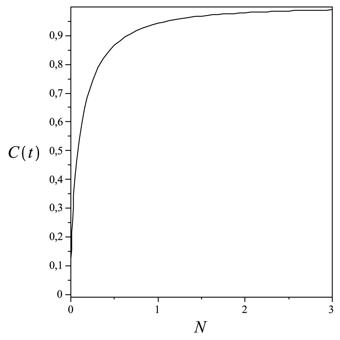
   Figure 1: Concurrence as function of $N$, for $|\phi_{1}\rangle$  as the initial state.

2. If we now consider $|\phi_{2}\rangle$ as the initial state, we get the solution of the master equation given by:

   $$\rho(t)=\begin{pmatrix}0&0&0&0\\ 0&1&0&0\\ 0&0&0&0\\ 0&0&0&0\end{pmatrix}.$$ (16)

   This state is also an invariant state and its concurrence is independent of time: $C(\rho)=1.$

In the following sections we consider, as initial states, $|\phi_{3}\rangle$ or $|\phi_{4}\rangle$ , and also superpositions of the form $\varepsilon$ $|\phi_{1}\rangle+\sqrt{1-\varepsilon^{2}}$ $|\phi_{4}\rangle$ and $\varepsilon$ $|\phi_{2}\rangle+\sqrt{1-\varepsilon^{2}}$ $|\phi_{3}\rangle.$ The idea is to increase $\varepsilon$ and to study the effect of having an increased component in the DFS on the death time of the entanglement. For simplicity, we assume $\gamma=1$, and $\psi=0$.

IV Solutions for $N=0$

1. The third initial state considered is $|\phi_{3}\rangle$. Initially its concurrence is: $C(\phi_{3}(0))=1.$ It  corresponds to a maximally entangled state.

   The solution of master equation for this initial condition and $N=0$ is given by:

   $$\rho(t)=\begin{pmatrix}(e^{2t}-1)e^{-2t}&0&0&0\\ 0&0&0&0\\ 0&0&e^{-2t}&0\\ 0&0&0&0\end{pmatrix}.$$ (17)

   Since the matrix $\rho(t)\widetilde{\rho}(t)$ has only one nonzero eigenvalue, in this case we use the separability criterion PERES . According to this criterion, the necessary condition for separability is that a matrix $\rho^{PT}$, obtained by partial transposition of $\rho$, should have only non-negative eigenvalues. In this particular case, we observe a negative eigenvalue for all times, so the state stays entangled, (Fig.2).

   

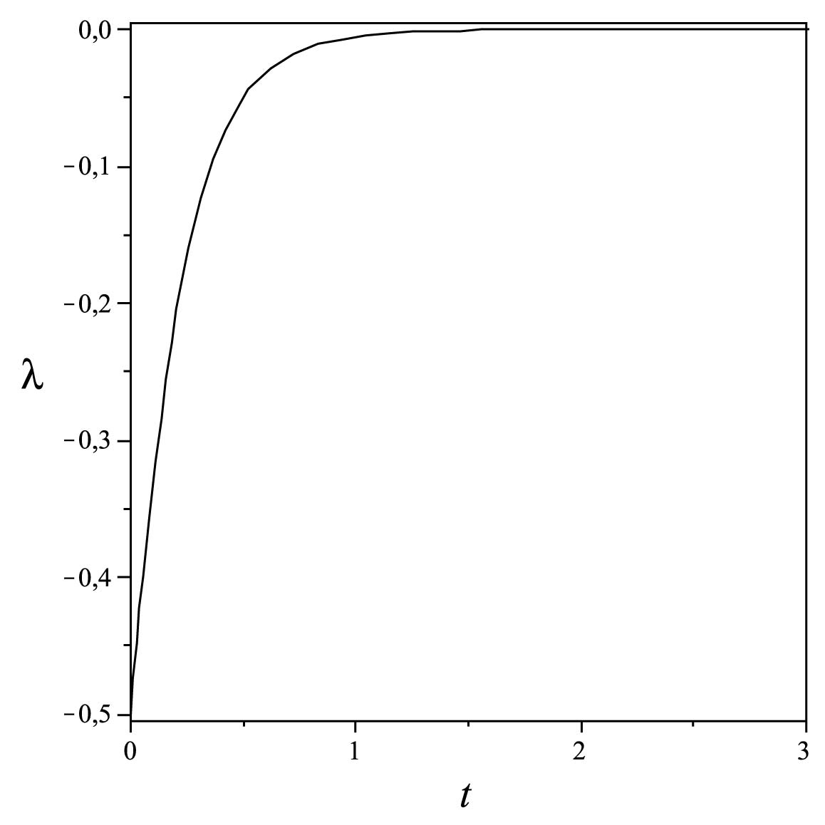
   Figure 2: Negative eigenvalue $(\lambda)$ of $\rho^{PT}$, for the separability criterion, for $|\phi_{3}\rangle$ as the initial state. This eigenvalue is always negative , indicating entanglement at all times.

2. Consider the initial state $|\phi_{4}\rangle$. Since $N=0$, $|\phi_{4}\rangle=|++\rangle$ and $C(\phi_{4}(0))=0$, since is a factorized state.

   The solution of master equation for this initial condition is given by:

   $$\rho(t)=\begin{pmatrix}(-1-2t+e^{2t})e^{-2t}&0&0&0\\ 0&0&0&0\\ 0&0&2te^{-2t}&0\\ 0&0&0&e^{-2t}\end{pmatrix},$$ (18)

   and its concurrence is $C(\rho(t))=0$.

3. Now, we consider an initial superposition of $|\phi_{1}\rangle$ and $|\phi_{4}\rangle$ : $|\Psi_{1}\rangle=\varepsilon$ $|\phi_{1}\rangle+\sqrt{1-\varepsilon^{2}}$ $|\phi_{4}\rangle$.

   As we increase $\varepsilon$, starting from $\varepsilon=0$, we increase the initial projection onto the DFS. For $\varepsilon=1$ the initial state is in the DFS plane.

   For $N=0$  we have: $|\Psi_{1}\rangle=\varepsilon$ $|--\rangle+\sqrt{1-\varepsilon^{2}}$ $|++\rangle$. Its initial concurrence is $C(\Psi_{1}(0))=2\varepsilon\sqrt{1-\varepsilon^{2}}$.

   The solution of master equation for this initial condition with $N=0$ is given by:

   $$\rho(t)=\begin{pmatrix}\frac{(-2t-1+2t\varepsilon^{2}+\varepsilon^{2}+e^{2t})}{e^{2t}}&0&0&\frac{\varepsilon\sqrt{1-\varepsilon^{2}}}{e^{t}}\\ 0&0&0&0\\ 0&0&\frac{2t(1-\varepsilon^{2})}{e^{2t}}&0\\ \frac{\varepsilon\sqrt{1-\varepsilon^{2}}}{e^{t}}&0&0&\frac{(1-\varepsilon^{2})}{e^{2t}}\end{pmatrix},$$ (19)

   and the corresponding concurrence is given by:

   $$C(\rho) =\max\{0,2\rho_{14}-\rho_{33}\}$$ (20)

   $$=\max\{0,2((\varepsilon\sqrt{1-\varepsilon^{2}})e^{-t}-te^{-2t}(1-\varepsilon^{2}))\}$$ (21)

   which is shown in fig.3 for various values of $\varepsilon$:

   

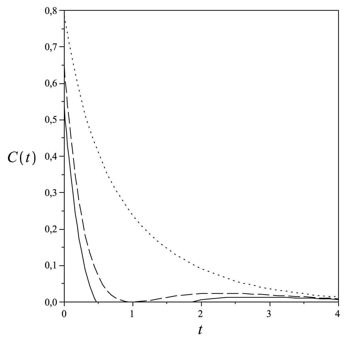
   Figure 3: Time evolution of the concurrence for initial $|\Psi_{1}\rangle$ with : $\varepsilon=0.28$ (solid line), $\varepsilon=0.345$ (dashed line), $\varepsilon=0.9$ (dotted line),

   For $\varepsilon=0$ and $\varepsilon=1$ , its concurrence is zero, therefore we have a non-entangled state. For $\varepsilon>0$ the initial entanglement decreases in time, and the system becomes disentangled (sudden death) at a time satisfying the relation:

   $$te^{-t}=\frac{\varepsilon}{\sqrt{1-\varepsilon^{2}}},$$ (22)

   For $0<\varepsilon<0.34525$  the equation (22) has two solutions, namely, $t_{d}$ when the system becomes separable, and $t_{r}\geq t_{d}$ when the entanglement revives. It should be noted that there is a critical $\varepsilon$ for which $t_{d}=t_{r}$. For $\ 0.34525<\varepsilon<1$ the above equation has no solution and the concurrence vanishes asymptotically in time.

   So, when we are ”not far” from $|\phi_{4}\rangle$ we observe a sudden death  and revival, but when we get ”near” $|\phi_{1}\rangle$  this phenomenon disappears. Fig.4 shows the behavior of the death and revival time as function of $\varepsilon.$

   

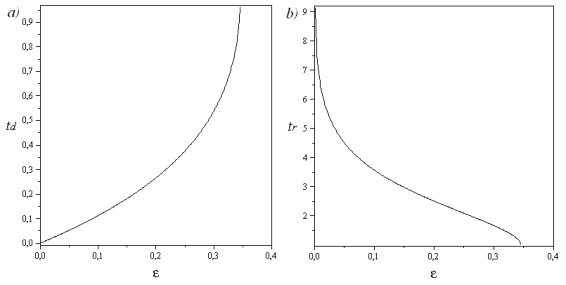
   Figure 4: a) The death time b)The revival time of the entanglement as a function of $\varepsilon$, with initial $|\Psi_{1}\rangle.$

4. Finally, we consider an initial superposition of $|\phi_{2}\rangle$ and $|\phi_{3}\rangle$ : $|\Psi_{2}(0)\rangle=\varepsilon$ $|\phi_{2}\rangle+\sqrt{1-\varepsilon^{2}}$ $|\phi_{3}\rangle$, which is independent of $N$.  So, like in the pervious cases, as we increase $\varepsilon$, starting from $\varepsilon=0$, we increase the initial projection onto the DFS. For $\varepsilon=1$ the initial state is in the DFS plane.

   For $N=0$  we have: $|\Psi_{2}\rangle=\frac{1}{\sqrt{2}}[(\varepsilon+\sqrt{1-\varepsilon^{2}})$ $|-+\rangle-(\varepsilon-\sqrt{1-\varepsilon^{2}})$ $|+-\rangle]$. Its initial concurrence is $C(\Psi_{2}(0))=|2\varepsilon^{2}-1|$.

   The solution of master equation for this initial condition is given by:

   $$\rho(t)=\begin{pmatrix}\frac{(e^{2t}-\varepsilon^{2}e^{2t}-1+\varepsilon^{2})}{e^{2t}}&0&0&0\\ 0&\varepsilon^{2}&\frac{\varepsilon\sqrt{1-\varepsilon^{2}}}{e^{t}}&0\\ 0&\frac{\varepsilon\sqrt{1-\varepsilon^{2}}}{e^{t}}&\frac{(1-\varepsilon^{2})}{e^{2t}}&0\\ 0&0&0&0\end{pmatrix},$$ (23)

   and the corresponding concurrence is:

   $$C(\rho) =\max\{0,|\rho_{33}-\rho_{22}|\}$$ (24)

   $$=\max\{0,e^{-2t}|\varepsilon^{2}e^{2t}-1+\varepsilon^{2}|\},$$ (25)

   which is shown in fig.5.

   

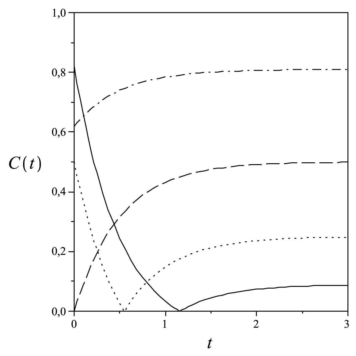
   Figure 5: Time evolution of the concurrence with intial $|\Psi_{2}\rangle$ , for : $\varepsilon=0.3$ (solid line), $\varepsilon=0.5$ (dotted line), $\varepsilon=0.707$ (dashed line), $\varepsilon=0.9$ (dash dotted line)

   For $0<\varepsilon<0.707$ the initial entanglement decreases in time, and the system becomes disentangled instantaneously, at a time given by:

   $$t=\frac{1}{2}\ln(\frac{1-\varepsilon^{2}}{\varepsilon^{2}}).$$ (26)

   However, at the same time, the entanglement revives reaching asymptotically its stationary value.(fig. 6)

   

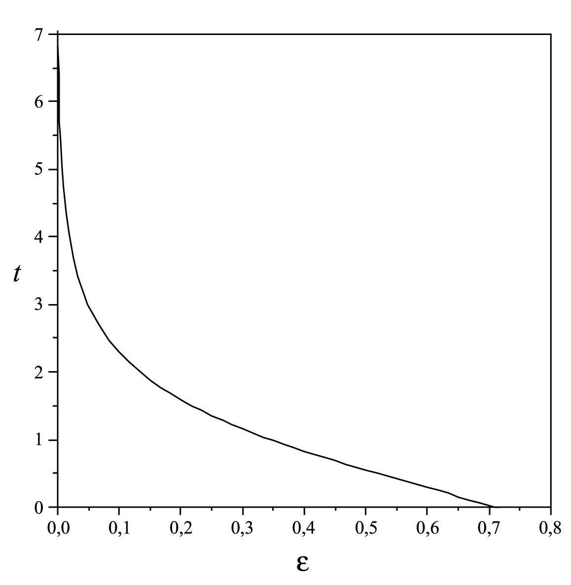
   Figure 6: Death-revival time as given by eq 26 , versus $\varepsilon.$

   When we approach the decoherence free subspace  this phenomenon disappears.

Next, we treat the cases with $N>0.$

V Solutions for $N\neq 0$

In general the solution of master equation for $|\phi_{3}\rangle$ , $|\phi_{4}\rangle$ and $|\Psi_{1}\rangle$  as initial condition and $N\neq 0$, has the following form:

$$\rho(t)=\begin{pmatrix}\rho_{11}&0&0&\rho_{14}\\ 0&0&0&0\\ 0&0&\rho_{33}&0\\ \rho_{41}&0&0&\rho_{44}\end{pmatrix},$$

and written at the standard basis, has the same structure as in  (12). Its concurrence is given by: $C(\rho)=max\{0,C1(\rho),C2(\rho)\}$, with the explicit expressions for $C1(\rho)$ and $C2(\rho)$ are given by:

$$C1(\rho) =2(\frac{\rho_{33}}{2}$$

$$-\sqrt{\frac{(\rho_{11}N+\rho_{44}(N+1)+2\rho 14\sqrt{N(N+1)})}{2N+1}}$$

$$\times\sqrt{\frac{(\rho_{44}N+\rho_{11}(N+1)-2\rho 14\sqrt{N(N+1)})}{2N+1}}),$$ (27)

$$C2(\rho) =2(\frac{|\sqrt{N(N+1)}(\rho_{11}-\rho_{44})+\rho_{14}|}{2N+1}-\frac{\rho_{33}}{2}).$$ (28)

On the other hand, for the initial condition $|\Psi_{2}\rangle$ , the corresponding expressions for the density matrix and concurrence are:

$$\rho(t)=\begin{pmatrix}\rho_{11}&0&0&\rho_{14}\\ 0&\rho_{22}&\rho_{23}&0\\ 0&\rho_{32}&\rho_{33}&0\\ \rho_{41}&0&0&\rho_{44}\end{pmatrix},$$

$$C1(\rho) =|\rho_{33}-\rho_{22}|$$

$$-2\sqrt{\frac{N(\rho_{11}+\rho_{44})+\rho_{44}+2\rho_{14}\sqrt{N(N+1)}}{2N+1}}$$

$$\times\sqrt{\frac{N(\rho_{11}+\rho_{44})+\rho_{11}-2\rho_{14}\sqrt{N(N+1)}}{2N+1}},$$ (29)

$$C2(\rho) =\frac{2}{2N+1}|\sqrt{N(N+1)}(\rho_{11}-\rho_{44})+\rho_{14}|$$

$$-\sqrt{(\rho_{22}-2\rho_{23}+\rho_{33})(\rho_{22}+2\rho_{23}+\rho_{33})}$$ (30)

1. Next, we consider again the case for initial $|\phi_{3}\rangle$ , but for $N\neq 0$. The concurrence is: $C(\rho)=max\{0,C1(\rho),C2(\rho)\}$, with its initial value $C(\phi_{3}(0))=1$.

   In fig.7, we show $C(t)$ versus time for various values of $N$. We observe sudden death in a finite time, then the concurrence remains zero for a period of time until  the entanglement revives, and the concurrence reaches asymptotically its stationary value. Notice that this time period increases with $N.$

   

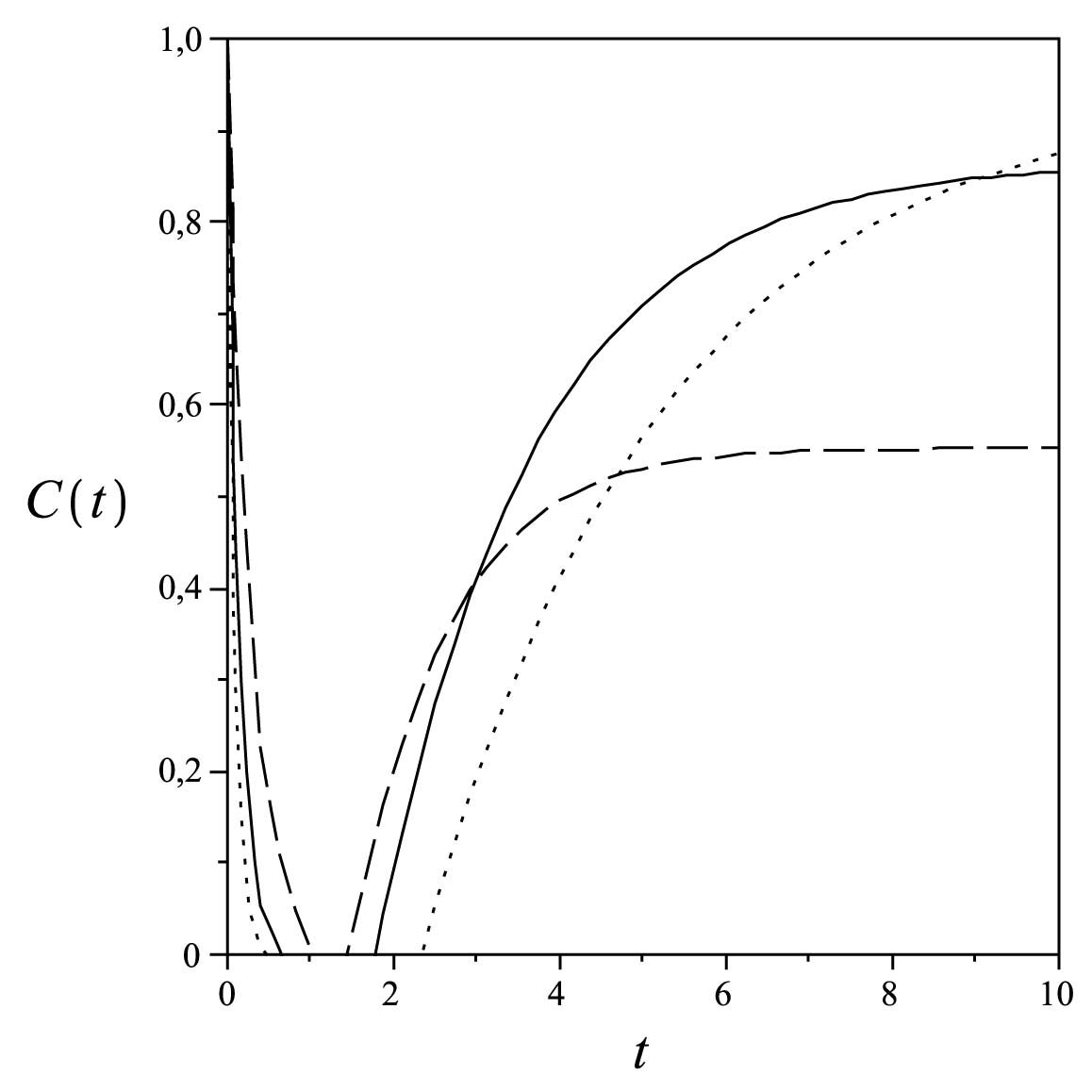
   Figure 7: Time evolution of concurrence for initial $|\phi_{3}\rangle$ , with: N=0.1 (dashed line), N=0.5 (solid line), N=1 (dotted line).

   In the fig.8 we show the death and revival times versus N. They decrease and increase with N respectively.

   

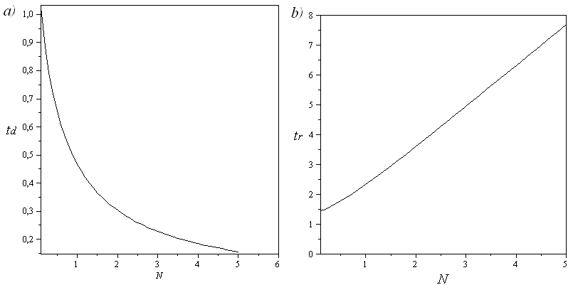
   Figure 8: a)Death time b) Revival time versus N for the initial state $\mid\phi_{3}\rangle.$

2. Consider $|\phi_{4}\rangle$ as an initial state. The concurrence, in this case, is: $C(\rho)=max\{0,C2(\rho)\}$, with $C2(\rho)$ defined by (28). Initially, it takes the value $C(\phi_{4}(0))=\frac{2\sqrt{N(N+1)}}{2N+1}.$ The behavior of concurrence is similar as in $|\phi_{3}\rangle$. The initial entanglement quickly decays to zero, getting disentanglement for a finite time interval , then the entanglement revives and asymptotically it reaches its stationary value.

   However, unlike the case with initial state $|\phi_{3}\rangle$, the death time first increases reaching a critical $N=0.421$, then decreases, as shown in Fig 9. The revival time has the same behavior as in $|\phi_{3}\rangle$.

   

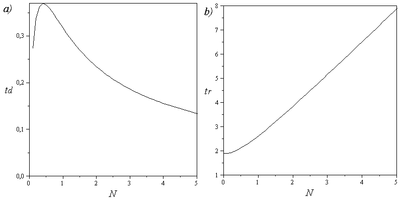
   Figure 9: Death (a) and Revival (b) times versus N for the initial state $\mid\phi_{4}\rangle.$

3. In the following case, we consider the superposition $|\Psi_{1}(t)\rangle=\varepsilon|\phi_{1}\rangle+\sqrt{1-\varepsilon^{2}}|\phi_{4}\rangle$ as the initial state. The solution of master equation for this initial condition depends on $\varepsilon$ and $N$ and also its concurrence, which is: $C(\rho)=\max\{0,C2(t)\}$, where $C2(t)$ is in 28. Since $C1(t)$ is always negative, the only contribution to the concurrence comes from $C2(t)$, . Its initial value being $C(\Psi_{1}(0))=\frac{|2\varepsilon\sqrt{1-\varepsilon^{2}}+4\sqrt{N(N+1)}(\varepsilon^{2}-\frac{1}{2})|}{2N+1}$ , hence is it clear that for certain pairs of $N$ and $\varepsilon$, our initial state will be a non-separable one. In the Fig. 10  we show the time evolution of the concurrence for $N=0.1$ and several values of $\varepsilon$. For $\varepsilon=0$ and $\varepsilon=1$ we retrieve $|\phi_{4}\rangle$ and $|\phi_{1}\rangle$ respectively. For $0<\varepsilon<0.5$  the concurrence dies in a finite time, stays zero for a time interval and subsequently revives, going asymptotically to its stationary value. For values larger than $\varepsilon=0.5,$ there is no more sudden death, since we are getting ”close” to the DFS, and $C(t)$ goes asymptotically to its stationary value.

   

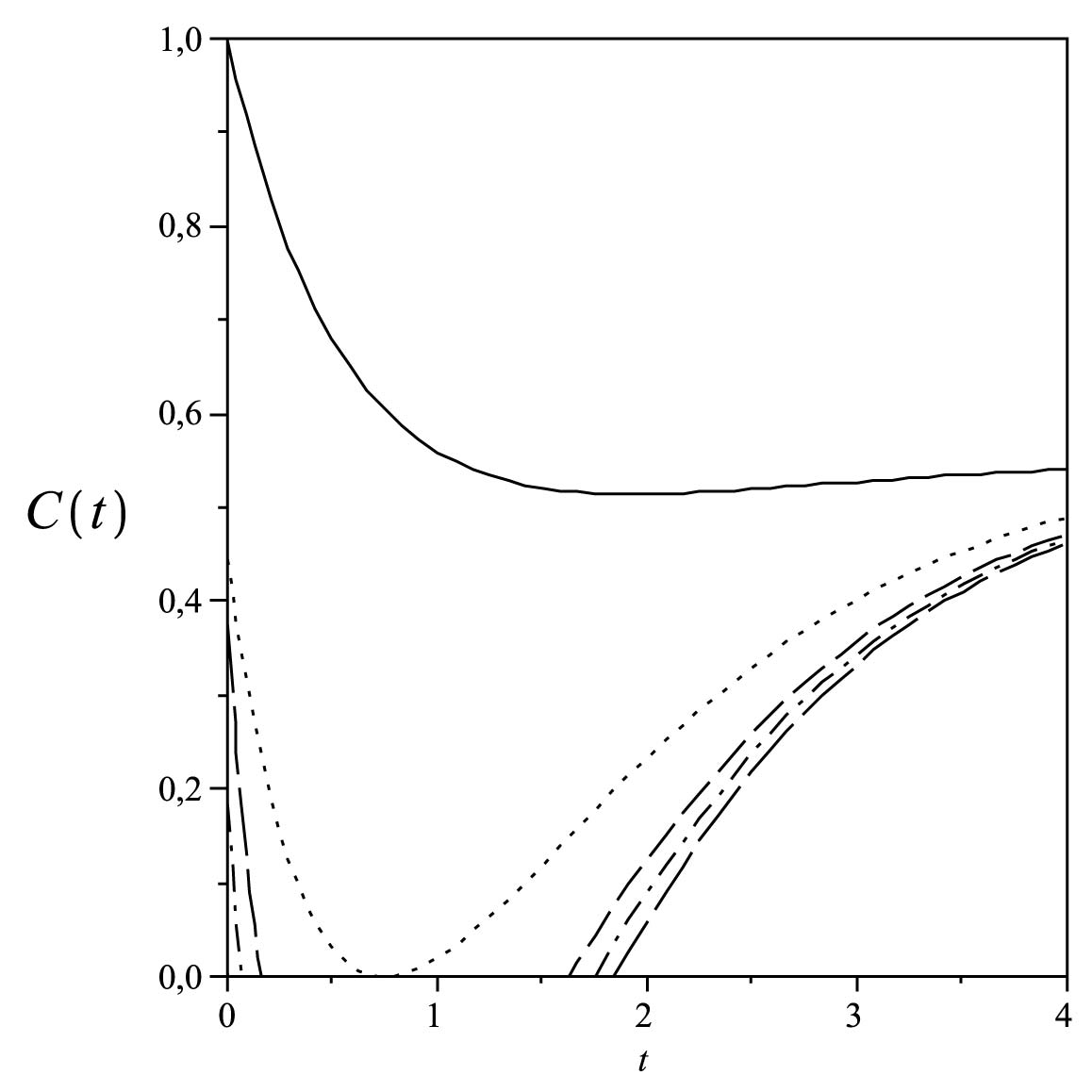
   Figure 10: Time evolution of Concurrence for $|\Psi_{1}(t)\rangle$ as initial state and $N=0.1$: $\varepsilon=0.1$ (long dashed line), $\varepsilon=0.2$ (dash dotted line), $\varepsilon=0.29$ (dashed line), $\varepsilon=0.5$ (dotted line), $\epsilon=0.9$ (solid line).

   The Figure 11 shows the death times versus $\varepsilon$ for $N=\{0,0.1,0.2\}$ . There is a curious effect, that for N$\neq$0, as we increase $\varepsilon,$ the death time first decreases and subsequently it behaves ”normally”, by increasing with $\varepsilon$. In the Fig. 12 we show the revival time as a function of $\varepsilon$ for the same values of $N$. In all cases the revival time decreases with $\varepsilon$.

   

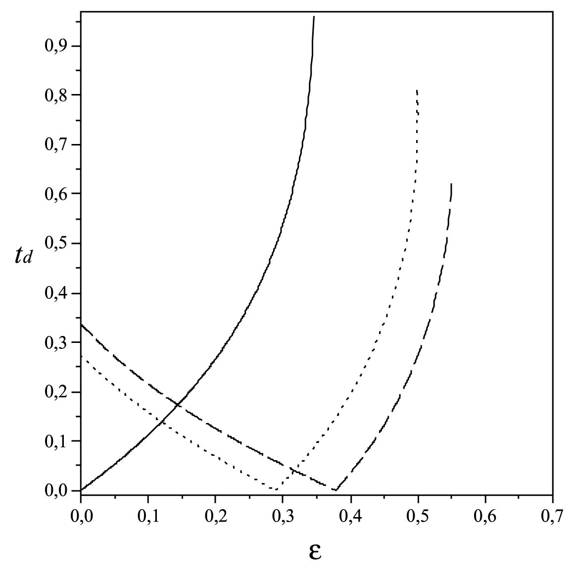
   Figure 11: Death time with initial $|\Psi_{1}\rangle$ and :$N=0$ (solid line), $N=0.1$ (dotted line), $N=0.2$ (dashed line)

   

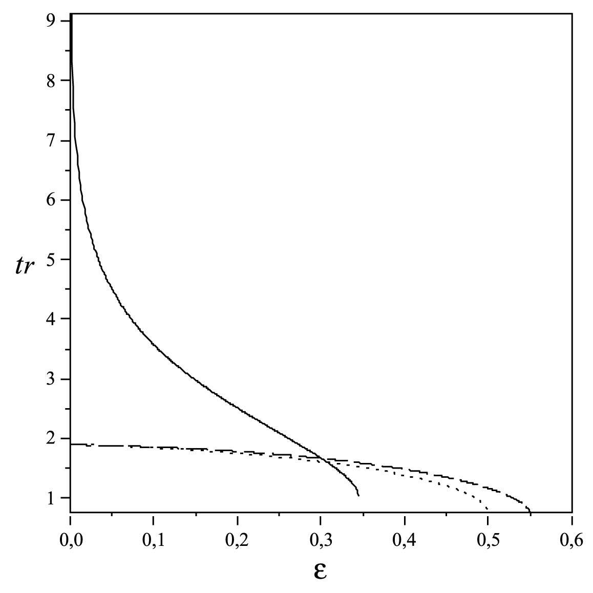
   Figure 12: Revival time with initial $|\Psi_{1}\rangle$ and :$N=0$ (solid line), $N=0.1$ (dotted line), $N=0.2$ (dashed line)

4. Finally, we consider the case with initial $|\Psi_{2}(t)\rangle=\varepsilon|\phi_{2}\rangle+\sqrt{1-\varepsilon^{2}}|\phi_{3}\rangle$ . Its concurrence is: $C(\rho(t))=\max\{0,C1(t),C2(t)\}$, with $C1(t)$ and $C2(t)$ defined in (29,30), and its initial value:$C(\Psi_{2}(0))=|2\varepsilon^{2}-1|$. Fig. 13. shows the time evolution of the concurrence with $N=0.1$ for several values of  $\varepsilon$ .

   

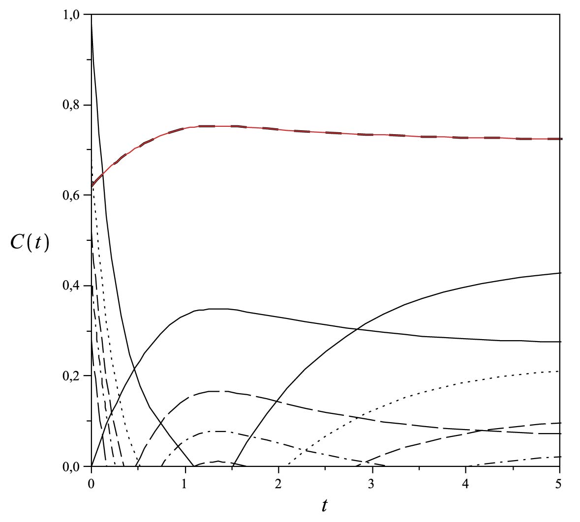
   Figure 13: Time evolution of concurrence for initial $|\Psi_{2}\rangle$ and: $\varepsilon=0.1$ (solid line), $\varepsilon=0.4$ (dotted line), $\varepsilon=0.49$ (dashed line), $\varepsilon=0.54$ (dash dotted line), $\varepsilon=0.6$ (long dashed line), $\varepsilon=0.9$ ( space dashed line),

   As we can see from the Fig. 13, this case is more complex, since there are more than one death and revival before reaching the critical value of $\varepsilon$. Such a situation has been described previously fi ; e4 . Like in the previous cases above a certain critical $\varepsilon$, when we get ”close” to the DFS, these effects disappear and $C(t)$ goes asymptotically to its stationary value.

VI Discussion

The first and most obvious observation is that if we start with an initial state that is in the DFS plane, the local and non-local coherences are not affected by the environment, thus it experiences no decoherence and the concurrence is constant in time. It does increase with the squeeze parameter N (in the case of initial $|\phi_{1}\rangle$), getting maximum entanglement for N$\rightarrow\infty.$ So this reservoir is not acting as a thermal one, in the sense that introduces $\operatorname{rand}$omness. On the contrary, a common squeezed bath tends to enhance the entanglement, as we increase the parameter N.

This is clear if we observe that for N$\rightarrow\infty$, $|\phi_{1}\rangle\rightarrow\frac{1}{\sqrt{2}}(|++\rangle+|--\rangle)$, which is a Bell state. On the other hand, if we start with the initial state $|\phi_{2}\rangle$, this state is independent of N and it is also maximally entangled, so C=1 for all times and all N´s.

Now, we consider other situations with initial states outside the DFS:

For N=0, $|\phi_{1}\rangle\rightarrow|--\rangle;|\phi_{4}\rangle\rightarrow|++\rangle$ while $|\phi_{2}\rangle$ and $|\phi_{3}\rangle$ are independent of N and represent the antisymmetrical singlet and one of the triplet states, respectively.

If our initial state is $|\phi_{3}\rangle$, the initial concurrence is C(t=0)=1, and for the steady state, C(t=$\infty$)=0. On the other hand, from the negativity of the eigenvalues of $\rho^{PT}$ (Peres-Horodecki criteria), we know that the state is entangled for all times, so presumably  the concurrence versus time is a smooth curve starting from 1 and going asymptotically to zero.

For an initial $|\phi_{4}\rangle=|++\rangle$, of course C(t=0)=0, since we have a factorized state. Since this initial state is symmetrical, the steady state is $|\phi_{1}\rangle=|--\rangle$, which is also a factorized state with C(t=$\infty$)=0. Our analysis shows that C(t)=0 for all times.

Finally, if we have initial states of the form $|\Psi_{1}\rangle=\varepsilon|\phi_{1}\rangle+\sqrt{1-\varepsilon^{2}}|\phi_{4}\rangle=\varepsilon$ $|--\rangle+\sqrt{1-\varepsilon^{2}}$ $|++\rangle$ or $|\Psi_{2}\rangle=\varepsilon|\phi_{2}\rangle+\sqrt{1-\varepsilon^{2}}|\phi_{3}\rangle=\frac{1}{\sqrt{2}}[(\varepsilon+\sqrt{1-\varepsilon^{2}})$ $|-+\rangle-(\varepsilon-\sqrt{1-\varepsilon^{2}})$ $|+-\rangle]$, there is sudden death if $0<\varepsilon<0.34525$ and $0<\varepsilon<0.707$ respectively. Obviously, when we get ”near” the DFS, that is $\varepsilon$ gets larger than zero, the sudden death times become larger up to some critical value, for which  the death time becomes infinite and we no longer observe the sudden death. Thus, we have related directly the local decoherence with the disentanglement.

Another interesting feature is the revival. For the $|\Psi_{1}\rangle$ case, after a finite time period, the entanglement ”revives”, and the concurrence reaches asymptotically its steady state value. This time gap becomes smaller for larger $\varepsilon$ until we reach $\varepsilon=0.34525$ . At this point, the two times merge and beyond that, there is no longer sudden death nor revival.

On the other hand, for the $|\Psi_{2}\rangle$ case, the sudden death and revival happen simultaneously, thus the above mentioned time period vanishes. The phenomena of one or periodical revivals have been obtained before, but always in the context of one single reservoir connecting both atoms, like in the present case fi ; fi2 ; e4 .

In the N$\neq 0$ case, we also observe sudden death and revivals, up to a certain ”distance” to the DFS ( or more precisely, up to a certain critical value of $\varepsilon$).

However, there are certain differences with the N=0 case.

For the initial state $|\phi_{4}\rangle$, the death time versus N first increases for small values of N, and for N$\gtrsim 0.421$, it tends to decrease. A possible interpretation of the increase is the following one:

$|\phi_{4}\rangle$=$\frac{1}{\sqrt{N^{2}+M^{2}}}(M|++\rangle-N|--\rangle)=\frac{N}{\sqrt{N^{2}+M^{2}}}(\sqrt{1+\frac{1}{N}}|++\rangle-|--\rangle)$, so that the ratio of the probabilities of the double excited and the ground states goes as $(1+\frac{1}{N}.)$

On the other hand, the squeezed vacuum has only components for the even number of photons, so the interaction between our system and the reservoir goes by pairs of photons. Now, for very small N, the average photon number is also small, so the predominant interaction with the reservoir will be the doubly excited state that would tend to decay via two photon spontaneous emission.. Now in the $|\phi_{4}\rangle$ case, the population of the $|++\rangle$ goes down with N, meaning that the interaction with the reservoir goes also down with N and therefore, the death time will necessarily increase with N, which describes qualitatively the first part of the curve (fig 9-a). On the other hand, as we increase the average photon number N, other processes like the two photon absorption will be favored, and since there will be more photons and the $|--\rangle$  population tends to increase with N, this will enhance the system-bath interaction and therefore the death of the entanglement will occur faster, or the death time will decrease.

In the $|\phi_{3}\rangle$ case, initially there is no $|++\rangle$ component, thus we expect a higher initial death time. However this case is different from the previous one in the sense that the state is independent of N, so there is no initial increase. However, as the state evolves in time, $|++\rangle$ and $|--\rangle$ components will build up and the argument for the decrease of the death time with N follows the same logic as in the previous case.(fig 8-a).

VI.1 Acknowledgements

MH was supported by a Conicyt grant.

M.O was supported by Fondecyt # 1051062.

The authors thank Prof. Sascha Wallentowitz for useful discussions.

VII APPENDIX

In the representation spanned by $\{|\phi_{1}\rangle,|\phi_{2}\rangle,|\phi_{3}\rangle,|\phi_{4}\rangle\}$, the solution of master equation (6) is:

$$\rho_{11}(t) =\frac{4}{\sqrt{N(N+1)}(8N+4)}\{[-(2N+1)(\rho_{44}(0)+\rho_{33}(0))$$

$$\times\sqrt{\frac{N(N+1)}{4}}+(\rho_{44}(0)+\rho_{33}(0)))N^{2}$$

$$+(\rho_{44}(0)+\rho_{33}(0))N+\frac{1}{4}\rho_{44}(0)]e^{-2t(\sqrt{N}+\sqrt{N+1})^{2}}$$

$$+[-(2N+1)(\rho_{44}(0)+\rho_{33}(0))\sqrt{\frac{N(N+1)}{4}}$$

$$-(\rho_{44}(0)+\rho_{33}(0)))N^{2}-(\rho_{44}(0)+\rho_{33}(0))N$$

$$-\frac{1}{4}\rho_{44}(0)]e^{-2t(\sqrt{N}-\sqrt{N+1})^{2}}$$

$$+(2N+1)(\rho_{44}(0)+\rho_{33}(0)+\rho_{11}(0))\sqrt{N(N+1)}\}$$

$$\rho_{12}(t)=\rho_{12}(0)$$

$$\rho_{13}(t) =\frac{12e^{-(2N+1)t}}{\sqrt{N}(24N^{3}+36N^{2}+10N-1)}[-\frac{2}{3}(N+\frac{1}{2})$$

$$\times(N\sqrt{N+1}+\frac{1}{4}\sqrt{2N+1}\sqrt{2N^{2}+N})$$

$$\times(\rho_{43}(0)-e^{i\Psi}\rho_{34}(0))e^{t\frac{(-\sqrt{2N^{2}+N}(2N+1)+4N\sqrt{N+1}\sqrt{2N+1})}{\sqrt{2N^{2}+N}}}$$

$$-\frac{2}{3}(N+\frac{1}{2})(N\sqrt{N+1}-\frac{1}{4}\sqrt{2N+1}\sqrt{2N^{2}+N})$$

$$\times(e^{i\Psi}\rho_{34}(0)+\rho_{43}(0))e^{-t\frac{(\sqrt{2N^{2}+N}(2N+1)+4N\sqrt{N+1}\sqrt{2N+1})}{\sqrt{2N^{2}+N}}}$$

$$+(-\frac{1}{3}(N+\frac{1}{2})\rho_{34}(0)e^{i\Psi}+\rho_{13}(0)(N^{2}+N-\frac{1}{12}))$$

$$\times\sqrt{2N+1}\sqrt{2N^{2}+N}+\frac{4}{3}(N+\frac{1}{2})\sqrt{N+1}\rho_{43}(0)]$$

$$\rho_{14}(t) =\frac{8e^{-(2N+1)t}}{(2N+1)(12N^{2}+12N-1)}[e^{-(2N+1+4\sqrt{N(N+1)})t}$$

$$\times(-\frac{1}{2}(N+\frac{1}{2})(2\rho_{44}(0)+\rho_{33}(0))\sqrt{N(N+1)}$$

$$+(\frac{1}{2}\rho_{44}(0)+\rho_{33}(0))(N^{2}+N)+\frac{1}{8}\rho_{44}(0))$$

$$-e^{-(2N+1-4\sqrt{N(N+1)})t}(\frac{1}{2}(N+\frac{1}{2})$$

$$\times(2\rho_{44}(0)+\rho_{33}(0))\sqrt{N(N+1)}$$

$$+(\frac{1}{2}\rho_{44}(0)+\rho_{33}(0))(N^{2}+N)+\frac{1}{8}\rho_{44}(0))$$

$$+\frac{3}{2}(\sqrt{2N+1}\rho_{14}(0)(N^{2}+N-\frac{1}{12})\sqrt{2N^{2}+N}$$

$$+\frac{2}{3}(N+\frac{1}{2})(2\rho_{44}(0)+\rho_{33}(0))N\sqrt{N+1})]$$

$$\rho_{21}(t)=\rho_{21}(0)$$

$$\rho_{22}(t)=\rho_{22}(0)$$

$$\rho_{23}(t)=\rho_{23}(0)e^{-(2N+1)t}$$

$$\rho_{24}(t)=\rho_{24}(0)e^{-(2N+1)t}$$

$$\rho_{31}(t) =\frac{-8e^{-i\Psi}e^{-(2N+1)t}}{\sqrt{N}(24N^{3}+36N^{2}+10N-1)}[(N\sqrt{N+1}{}$$

$${}-\frac{1}{4}\sqrt{2N+1}\sqrt{2N^{2}+N})(N+\frac{1}{2}){}$$

$${}\times(e^{i\Psi}\rho_{34}(0)+\rho_{43}(0))e^{\frac{-(((2N+1)t+I\Psi)\sqrt{2N^{2}+N}+4tN\sqrt{N+1}\sqrt{2N+1}}{\sqrt{2N^{2}+N}}}{}$$

$${}+e^{i\Psi}(N+\frac{1}{2})(N\sqrt{N+1}+\frac{1}{4}\sqrt{2N+1}\sqrt{2N^{2}+N}){}$$

$${}\times(e^{i\Psi}\rho_{34}(0)-\rho_{43}(0))e^{\frac{-(((2N+1)t+I\Psi)\sqrt{2N^{2}+N}-4tN\sqrt{N+1}\sqrt{2N+1}}{\sqrt{2N^{2}+N}}}{}$$

$${}-\frac{2}{3}\sqrt{2N+1}\sqrt{2N^{2}+N}(\rho_{31}(0)e^{i\Psi}(N^{2}+N-\frac{1}{2}){}$$

$${}-\frac{1}{3}(N+\frac{1}{2})\rho_{43}(0))-(2N+1)N\sqrt{N+1}\rho_{34}(0)e^{i\Psi}]$$

$$\rho_{32}(t)=\rho_{32}(0)e^{-(2N+1)t}$$

$$\rho_{33}(t) =\frac{1}{2}[e^{-2t(\sqrt{N}-\sqrt{N+1})^{2}}(\rho_{33}(0)+\rho_{44}(0)\frac{(N+1)}{\sqrt{N(N+1)}})$$

$$+[e^{-2t(\sqrt{N}+\sqrt{N+1})^{2}}(\rho_{33}(0)-\rho_{44}(0)\frac{(N+1)}{\sqrt{N(N+1)}}]$$

$$\rho_{34}(t) =\frac{1}{2}(\rho_{34}(0)-e^{-i\Psi}\rho_{43}(0))e^{-2t(\sqrt{N}-\sqrt{N+1})^{2}}$$

$$+\frac{1}{2}(\rho_{34}(0)+e^{-i\Psi}\rho_{43}(0))e^{-2t(\sqrt{N}+\sqrt{N+1})^{2}}$$

$$\rho_{41}(t) =\frac{12e^{-(2N+1)t}}{N\sqrt{N+1}(2N+1)(12N^{2}+12N-1)}[\frac{1}{3}N\sqrt{N+1}$$

$$\times(-(2N+1)(\frac{\rho_{33(0)}}{2}+\rho_{44}(0))\sqrt{N(N+1)}$$

$$+(2\rho_{33}(0)+\rho_{44}(0))(N^{2}+N)$$

$$+\frac{\rho_{44}(0)}{4})e^{-(2N+1+4\sqrt{N(N+1)})t}-\frac{1}{3}N\sqrt{N+1}$$

$$\times((2N+1)(\frac{\rho_{33(0)}}{2}+\rho_{44}(0))\sqrt{N(N+1)}$$

$$+(2\rho_{33}(0)+\rho_{44}(0))(N^{2}+N)$$

$$+\frac{\rho_{44}(0)}{4})Ne^{-(2N+1-4\sqrt{N(N+1)})t}$$

$$+\sqrt{N(N+1)}(\sqrt{2N+1}\rho_{41}(0)(N^{2}-\frac{1}{12}+N)$$

$$\times\sqrt{2N^{2}+N}+\frac{4}{3}(N+\frac{1}{2})N\sqrt{N+1}N$$

$$\times(\frac{\rho_{33}(0)}{2}+\rho_{44}(0)))]$$

$$\rho_{42}(t)=\rho_{42}(0)e^{-(2N+1)t}$$

$$\rho_{43}(t) =\frac{1}{2}(\rho_{43}(0)-e^{i\Psi}\rho_{34}(0))e^{-2t(\sqrt{N}-\sqrt{N+1})^{2}}$$

$$+\frac{1}{2}(\rho_{43}(0)+e^{i\Psi}\rho_{34}(0))e^{-2t(\sqrt{N}+\sqrt{N+1})^{2}})$$

$$\rho_{44}(t) =(\frac{\rho_{44}(0)}{2}-\frac{\sqrt{N(N+1)}}{2N+1}\rho_{33}(0))e^{-2t(\sqrt{N}+\sqrt{N+1})^{2}}$$

$$+(\frac{\rho_{44}(0)}{2}+\frac{\sqrt{N(N+1)}}{2N+1}\rho_{33}(0))e^{-2t(\sqrt{N}-\sqrt{N+1})^{2}}$$

References

- (1) C.H.Bennett, G.Brassard, C.Crepeau, R.Jozsa, A.Peres, W.K.Wooters, Phys.Rev.Lett, 70, 1895 (1993)
- (2) A.K.Ekert, Phys.Rev.Lett, 67, 661 (1991); D.Deutsch, A.K.Ekert, R.Jozsa, C.Macchiavello, S.Popescu, A.Sanpera, Phys.Rev.Lett, 77, 2818 (1996)
- (3) C.H.Bennett, S.J.Wiesner, Phys.Rev.Lett, 69, 2881 (1992)
- (4) T.Yu and J.H.Eberly, Phys.Rev.Lett, 93, 140404 (2004)
- (5) T.Yu and J.H.Eberly, Phys.Rev.Lett, 97, 140403 (2006)
- (6) T.Yu and J.H.Eberly, Opt.Commun, 264, 393 (2006)
- (7) M.P.Almeida, F.de Melo, M.Hor-Meyll, A.Salles, S.P.Wallborn, P.H.Souto Ribeiro, L.Davidovich, e-print arXiv:quant-ph/0701184; M.F.Santos, P.Milman, L.Davidovich, N.Zagury, Phys.Rev.A, 73, 040305 (R) (2006)
- (8) D.Mundarain and M. Orszag, Phys. Rev. A 75, 040303(R) (2007).
- (9) D.Mundarain and M. Orszag, J.Stephany, Phys. Rev. A 74, 052107 (2006).
- (10) M.Orszag, Quantum Optics, (2nd ed, Springer Verlag,Berlin, 2007 )
- (11) W.K.Wootters, Phys. Rev. Lett 80, 2245 (1998).
- (12) J.Wang, H.Batelaan, J.Podany, A.F.Starace, J.Phys.B, 39, 4343 (2006)
- (13) M.Ikram, Fu-li Li, S.Zubairy, Phys.Rev.A, 75, 062336 (1007)
- (14) Asher Peres, Phys. Rev Lett 77, 1413 (1996)
- (15) Z.Ficek, R.Tanas, Phys.Rev.A, 74, 024304 (2006)
- (16) R.Tanas, Z.Ficek, J.Opt.B: Quantum.Semiclass, 6, S610 (2004)
- (17) T.Yu, J.H.Eberly, e-print arXiv:quant-ph/0703083