Transmission code optimization method for incoherent scatter radar

Zusammenfassung

When statistical inversion of a lag profile is used to determine an incoherent scatter target, the posterior variance of the estimated target can be used to determine how well a certain set of transmission codes perform. In this work we present an incoherent scatter radar transmission code optimization search method suitable for different modulation types, including binary phase, polyphase and amplitude modulation. We find that the combination of amplitude and phase modulation provides better performance than traditional binary phase coding, in some cases giving better accuracy than alternating codes.

Incoherent scatter radar lag profile measurements can be deconvolved using statistical inversion with arbitrary range and time resolution as shown by Virtanen et al. (2007a). In this case, the transmission does not need to be completely free of ambiguities. The only important factor is the variance of the estimated target autocorrelation function. Even though alternating codes are transmission sequences that are optimal in terms of posterior variance when integrated over the code transmission cycle (Lehtinen, 1986), shorter and only slightly less optimal code groups are beneficial in many cases where an alternating code sequence is too long. Also, a shorter code group offers much more flexibility when designing radar experiments, e.g., making it easier to combine multiple different experiments in the same frequency channel and simplifying ground clutter removal. The use of short transmission codes is described in more detail in the companion paper by Virtanen et al. (2007b) submitted to this same issue.

We have previously studied the target estimation variance of a coherent target where the target backscatter is assumed to stay constant while the transmission travels through the target (Vierinen et al., 2006). We found using an optimization algorithm that a combination of amplitude and arbitrary phase modulation can achieve very close to optimum coding (the order $10^{-4}$ less than optimal in terms of normalized variance). In this study we apply an optimization method, similar to the one used for coherent targets, to find transmission codes that minimize the variance of incoherent target autocorrelation function estimates. We compare results of the optimization algorithm for several different modulation methods.

All formulas in this paper use discrete time, unless otherwise stated. All waveforms discussed are complex valued baseband signals. The ranges will be defined as round-trip time for the sake of simplicity.

1 General transmission code

A code with length $L$ can be described as an infinite length sequence with a finite number of nonzero bauds with phases and amplitudes defined by parameters $\phi_{k}$ and $a_{k}$. These parameters obtain values $\phi_{k}\in[0,2\pi]$ and $a_{k}\in[a_{\mathrm{min}},a_{\mathrm{max}}]$, where $k\in[1,\ldots,L]:k\in\mathbb{N}$. The reason why one might want to restrict the amplitudes to some range stems from practical constraints in transmission equipment. Usually, the maximum peak amplitude is restricted in addition to average duty cycle. Also, many systems only allow a small number of phases. The commonly used binary phase coding allows only two phases: $\phi_{k}\in\{0,\pi\}$.

By first defining $\delta(t)$ with $t\in\mathbb{Z}$ as

$$\delta(t)=\left\{\begin{array}[]{llr}1&\quad\mbox{when}&\quad t=0\\ 0&\quad\mbox{otherwise},&\end{array}\right.$$ (1)

we can describe an arbitrary baseband radar transmission envelope $\epsilon(t)$ as

$$\epsilon(t)=\sum_{k=1}^{L}a_{k}e^{i\phi_{k}}\delta(t-k+1).$$ (2)

We restrict the total transmission code power to be constant for all codes of similar length. Without any loss of generality, we set code power equal to code length

$$L=\sum_{t=1}^{L}|\epsilon(t)|^{2}.$$ (3)

This will make it possible to compare estimator variances of codes with different lengths. It is also possible to compare codes of the same length and different transmission powers by replacing $L$ with the relative transmission power.

2 Lag estimation variance

We will only discuss estimates of the target autocorrelation function $\sigma_{\tau}(r)$ with lags $\tau$ that are shorter than the length of a transmission code (here $r$ is the range in round-trip time, and it is discretized by the baud length). The lags are assumed to be non-zero multiples of the baud length of the transmission code. Autocorrelation function estimation variance is presented more rigorously in the companion paper by Lehtinen et al. (2007) submitted to the same special issue. The variance presented there also includes pulse-to-pulse and fractional lags, taking into account target post-integration as well.

Lag profile inversion is conducted using lagged products for the measured receiver voltage, defined for lag $\tau$ as

$$m_{\tau}(t)\equiv m(t)\,\overline{m(t+\tau)}.$$ (4)

As more than one code is used to perform the measurement, we index the codes with $c$ as $\epsilon^{c}(t)$. For convenience, we define a lagged product of the code as

$$\epsilon_{\tau}^{c}(t)\equiv\epsilon^{c}(t)\,\overline{\epsilon^{c}(t+\tau)}.$$ (5)

With the help of these two definitions, the lagged product measurement can be stated as a convolution of the lagged product of the transmission with the target autocorrelation function

$$m^{c}_{\tau}(t)=(\epsilon_{\tau}^{c}*\sigma_{\tau})(t)+\xi_{\tau}(t),$$ (6)

The equation also contains a noise term $\xi_{\tau}(t)$, which is rather complicated, as it also includes the unknown target $\sigma_{\tau}(r)$. This term is discussed in detail, e.g., by Huuskonen and Lehtinen (1996). In the case of low SNR, which is typical for incoherent scatter measurements, the thermal noise dominates and $\xi_{\tau}(t)$ can be approximated as a Gaussian white noise process defined as

$$\mathbf{E}\,\xi_{\tau}(i)\,\overline{\xi_{\tau}(j)}=\delta(i-j)\,s^{2},$$ (7)

where $s^{2}$ is the variance of the measurement noise.

In this case, the normalized measurement “noise power” of lag $\tau$ can then be approximated in frequency domain as

$$P_{\tau}\approx\int_{0}^{2\pi}\frac{N_{c}(L-\tau)}{\sum_{c=1}^{N_{c}}|\hat{\epsilon}_{\tau}^{c}(\omega)|^{2}}d\omega,$$ (8)

where $\hat{\epsilon}_{\tau}^{c}(\omega)=\mathcal{F}_{D}^{M}\{\epsilon_{\tau}^{c}(t)\}$ is a zero padded discrete Fourier transform of the transmission envelope with transform length $M\gg L$. $N_{c}$ is the number of codes in the transmission group and $L$ is the number of bauds in a code. Each code in a group is assumed to be the same length.

will not

For alternating codes of both Lehtinen (1986) and Sulzer (1993) type, $P_{\tau}=1$ for all possible values of $\tau$. For constant amplitude codes, this is the lower limit. On the other hand, if amplitude modulation is used, this is not the lower limit anymore, because in some cases more radar power can be used on certain lags, even though the average transmission power is the same.

To give an idea of how phase codes perform in general, Fig. 1 shows the mean lag noise power for random code groups at several different code and code group lengths. It is evident that when the code group is short and the code length is large, the average behaviour is not very good. On the other hand, when there is a sufficient number of codes in a group, the performance is fairly good even for randomly chosen code groups. Thus, we only need to worry about performance of short code groups that are sufficiently long.

3 Code optimization criteria

Nearly all practical transmission code groups result in such a vast search space that there is no possibility for an exhaustive search. As we cannot yet analytically derive the most optimal codes, except in a few selected situations, we must resort to numerical means. The problem of finding a transmission code with minimal estimation variance is an optimization problem and there exist a number of algorithms for approaching this problem numerically.

A typical approach is to define an optimization criteria $f(x)$ with a parameter vector $x$. The optimization algorithm then finds $x_{\mathrm{min}}$ that minimizes $f(x)$. In the case of transmission code groups, $x$ will contain the phase $\phi^{c}_{k}$ and amplitude $a^{c}_{k}$ parameters of each code in the code group

$$x=\{a_{1}^{1},...,a_{L}^{N_{c}},\phi_{1}^{1},...,\phi_{L}^{N_{c}}\}.$$ (9)

There are many different ways to define $f(x)$ in the case of transmission code groups, but a trivial one is a weighted sum of the normalized lag power $P_{\tau}$, with weights $w_{\tau}$ selected in such a way that they reflect the importance of that lag

$$f(x)=\sum_{\tau}w_{\tau}\,P_{\tau}.$$ (10)

In this paper, we set $w_{\tau}=1$ for all lags. This gives each lag an equal importance. This is a somewhat arbitrary choice of weights, in reality they should be selected in a way the reflects the importance of the lag in the experiment.

4 Optimization algorithm

As our search method will also have to work with codes that have a finite number of phases, we needed an algorithm that could also work with situations were an analytic or numerical derivative of $f(x)$ cannot be defined. We developed an algorithm for this specific task, which belongs to the class of random local algorithms (Lewis and Papadimitriou, 1997). Another well known algorithm belonging to the same class is simulated annealing (Kirkpatrick et al., 1983), which has some similarities to the optimization algorithm that we used.

The random local optimization algorithm is fairly efficient at converging to a minima of $f(x)$ and it can also to some extent jump out of local minima. In practice, it is faster to restart the optimization search with a different random initial parameter set, in order to efficiently locate the minima of $f(x)$ that can then be compared the different optimization runs.

A simplified description of our code search algorithm that searches for local minima of $f(x)$ is as follows:

1. Randomize parameters in $x$.

2. For a sufficient number of steps, randomize a new value for one of the elements of $x$ and accept the change if $f(x)$ is improved.

3. Randomize all parameters $x$, accept the change if $f(x)$ is improved.

4. If sufficient convergence to a local minima of $f(x)$ has been achieved, save $x$ and goto step 1. Otherwise go to step 2. The location of the minima can be further fine tuned using gradient-based methods, if a gradient is defined for $f(x)$.

In practice, our algorithm also included several tunable variables that were used in determining the convergence of $f(x)$ to a local minima. Also, the number of local minima to search for depends a lot on the number of parameters in the problem. In many cases we are sure that the global minima was not even found as the number of local minima was so vast.

5 Optimization results

In order to demonstrate the usefulness of the optimization method, we searched for code groups that use three different types of modulation: binary phase modulation, polyphase modulation, and the combination of amplitude and polyphase modulation, which we shall refer to as general modulation. In this example, we used $a_{k}=1$ for the constant amplitude modulations and allowed amplitudes in the range $a_{k}\in[0,2]$ for general modulation codes, while still constraining the total transmission code power in both cases to be the same.

The results are shown in Fig. 1. In this case the results are shown in terms of mean lag noise power $P=(L-1)^{-1}\sum_{\tau}P_{\tau}$. It is evident that significant improvement can be achieved when the code group length is short. For longer code groups, the optimized groups do not different that much from random code groups. Also, one can see that optimized polyphase codes are somewhat better than binary phase codes; ultimately general phase codes are better than polyphase codes – in some cases the mean lag noise power is actually better than unity. The reason for this is that amplitude modulation allows the use of more power for measuring some lags, in addition to allowing more freedom in removing range ambiguities. It should also be noted, that when the code or code group length is increased, the difference between modulation methods also becomes less significant.

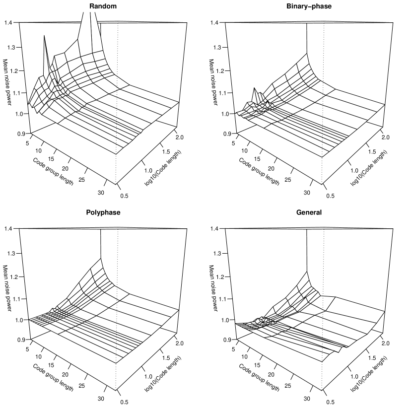
Abbildung 1: The mean lag noise power for random codes, optimized binary phase codes, optimized polyphase codes and optimized amplitude $a_{k}\in[0,2]$ and arbitrary phase modulated (general modulation) codes. The largest improvements are achieved for short code groups. Also, it is clear that the combination of amplitude and phase modulation provides the best lag variance.

We have introduced an optimization method suitable for searching optimal transmission codes when performing lag profile inversion. General radar tranmission coding, i.e., modulation that allows amplitude and arbitrary phase shifts, is shown to perform better than plain binary phase modulation. Amplitude modulation is shown to be even more effective than alternating codes, as the amplitude modulation allows the use of more radar power in a subset of the lags.

For sake of simplicity, we have only dealt with estimation variances for lags that are non-zero multiples of the baud length, with the additional condition that the lags are shorter than the transmission pulse length. It is fairly easy to extend this same methodology for more complex situations that, e.g., take into account target post-integration, fractional or pulse-to-pulse lags. This is done by modifying the optimization criterion $f(x)$.

In the cases that we investigated, the role of the modulation method is important when the code length is short. When using longer codes or code groups, the modulation becomes less important. Also, the need for optimizing codes becomes smaller when the code group length is increased.

Further investigation of the high SNR case would be beneficial and the derivation of variance in this case would be interesting, albeit maybe not as relevant in the case of incoherent scatter radar.