Personal Recommendation via Modified Collaborative Filtering

Abstract

In this paper, we propose a novel method to compute the similarity between congeneric nodes in bipartite networks. Different from the standard cosine similarity, we take into account the influence of node’s degree. Substituting this new definition of similarity for the standard cosine similarity, we propose a modified collaborative filtering (MCF). Based on a benchmark database, we demonstrate the great improvement of algorithmic accuracy for both user-based MCF and object-based MCF.

PACS numbers: 89.75.Hc, 87.23.Ge, 05.70.Ln

Key words: recommendation system, bipartite network, similarity, collaborative filtering

I Introduction

Recently, recommendation systems are attracting more and more attentions, because it can help users to deal with information overload, which is a great challenge in the modern society, especially under the exponential growth of the Internet 1 and the World-Wide-Web 2 . Recommendation algorithm has been used to recommend books and CDs at Amazon.com, movies at named Netflix.com, and news at VERSIFI Technologies (formerly AdaptiveInfo.com) 3 . The simplest algorithm we can use in these systems is global ranking method (GRM) 15 , which sorts all the objects in the descending order of degree and recommends those with highest degrees. GRM is not a personal algorithm and its accuracy is not very high because it does not take into account the personal preferences. Accordingly, various kinds of personal recommendation algorithms are proposed, for example, the collaborative filtering (CF) 4 ; 5 , the content-based methods 6 ; 7 , the spectral analysis 8 ; renjie , the principle component analysis 9 , the diffusion approach 15 ; 16 ; 18 ; ljg , and so on. However, the current generation of recommendation systems still requires further improvements to make recommendation methods more effective 3 . For example, the content analysis is practical only if the items have well-defined attributes and those attributes can be extracted automatically; for some multimedia data, such as audio/video streams and graphical images, the content analysis is hard to apply. The collaborative filtering usually provides very bad predictions/recommendations to the new users having very few collections. The spectral analysis has high computational complexity thus infeasible to deal with huge-size systems.

Thus far, the widest applied personal recommendation algorithm is CF 3 ; 10 . The CF has two categories in general, one is user-based (U-CF), which recommends the target user the objects collected by the users sharing similar tastes; the other is object-based (O-CF), which recommends those objects similar to the ones the target user preferred in the past. In this paper, we introduce a modified collaborative filtering (MCF), which can be implemented for both object-based and user-based cases and achieve much higher accuracy of recommendation.

II Method

We assume that there is a recommendation system which consists of $m$ users and $n$ objects, and each user has collected some objects. The relationship between users and objects can be described by a bipartite network. Bipartite network is a particular class of networks 15 ; 17 , whose nodes are divided into two sets, and connections among one set are not allowed. We use one set to represent users, and the other represents objects: if an object $o_{i}$ is collected by a user $u_{j}$, there is an edge between $o_{i}$ and $u_{j}$, and the corresponding element $a_{ij}$ in the adjacent matrix A is set as 1, otherwise it is 0.

In U-CF, the predicted score $v_{ij}$ (to what extent $u_{j}$ likes $o_{i}$), is given as :

$$v_{ij}=\sum^{m}_{l=1,l\neq{i}}s_{il}a_{jl},$$ (1)

where $s_{il}$ denotes the similarity between $u_{i}$ and $u_{l}$. For any user $u_{i}$, all $v_{ij}$ are ranked by values from high to low, objects on the top and have not been collected by $u_{i}$ are recommended.

How to determine the similarity between users? The most common approach taken in previous works focuses on the so-called structural equivalence. Two congeneric nodes (i.e. in the same set of a bipartite network) are considered structurally equivalent if they share many common neighbors. The number of common objects shared by users $u_{i}$ and $u_{j}$ is

$$c_{ij}=\sum^{n}_{l=1}a_{li}a_{lj},$$ (2)

which can be regarded as a rudimentary measure of $s_{il}$. Generally, the similarity between $u_{i}$ and $u_{j}$ should be somewhat relative to their degrees 11 . There are at least three ways previously proposed to measure similarity, as:

$$s_{ij}=\frac{2c_{ij}}{k(u_{i})+k(u_{j})},$$ (3)

$$s_{ij}=\frac{c_{ij}}{\sqrt{k(u_{i})k(u_{j})}},$$ (4)

$$s_{ij}=\frac{c_{ij}}{min(k(u_{i}),k(u_{j}))}.$$ (5)

The Eq.(3) is called Sorensen’s index of similarity (SI) 12 , which was proposed by Sorensen in 1948; the Eq.(4), called the cosine similarity, was proposed by Salton in 1983 and has a long history of the study on citation networks 11 ; the Eq.(5) is called Pearson correlation. Both the Eq.(4) and Eq.(5) are widely used in recommendation systems 3 ; 15 .

A common blemish of Eqs. (3)-(5) is that they have not taken into account the influence of object’s degree, so the objects with different degrees have the same contribution to the similarity. If user $u_{i}$ and $u_{j}$ both have selected object $o_{l}$, that is to say, they have a similar taste to the object $o_{l}$. Provided that object $o_{l}$ is very popular (the degree of $o_{l}$ is very large), this taste (the favor for $o_{l}$) is a very ordinary taste and it does not means $u_{i}$ and $u_{j}$ are very similar. Therefore, its contribution to $s_{ij}$ should be small. On the other hand, provided that object $o_{l}$ is very unpopular (the degree of $o_{l}$ is very small), this taste is a peculiar taste, so its contribution to $s_{ij}$ should be large. In other words, it is not very meaningful if two users both select a popular object, while if a very unpopular object is simultaneously selected by two users, there must be some common tastes shared by these two users. Accordingly, the contribution of object $o_{l}$ to the similarity $s_{ij}$ (if $u_{i}$ and $u_{j}$ both collected $o_{l}$) should be negatively correlated with its degree $k(o_{l})$. We suppose the object $o_{l}$’s contribution to $s_{ij}$ being inversely proportional to $k^{\alpha}(o_{l})$, with $\alpha$ a freely tunable parameter. The $s_{ij}$, consisted of all the contributions of commonly collected objects, is measured by the cosine similarity as shown in Eq. (4). Therefore, the proposed similarity reads:

$$s_{ij}=\frac{1}{\sqrt{k(u_{i})k(u_{j})}}\sum^{n}_{l=1}\frac{a_{li}a_{lj}}{k^{\alpha}(o_{l})}.$$ (6)

Note that, the influence of object’s degree can also be embedded into the other two forms, shown in Eq. (3) and Eq. (5), and the corresponding algorithmic accuracies will be improved too. Here in this paper, we only show the numerical results on cosine similarity as a typical example.

Figure 1: The degree distributions of users (left panel) and objects (right panel) in linear-log plot, where $P(k)$ denotes the cumulative degree distribution.

For any user-object pair $u_{i}$-$o_{j}$, if $u_{i}$ has not yet collected $o_{j}$, the predicted score can be obtained by using Eq. (1). Here we do not normalize Eq. (1), because it will not affect the recommendation list, since for a given target user, we need sort all her uncollected objects, and only the relative magnitude is meaningful. Note that, if two objects have exactly the same score, their order is randomly assigned. We call this method a modified collaborative filtering (U-MCF), for it belongs to the framework of U-CF.

III Numerical results

Using a benchmark data set namely MovieLens 13 , we can evaluate the accuracy of the current algorithm. The data consists of 1682 movies (objects) and 943 users. Actually, MovieLens is a rating system, where each user votes movies in five discrete ratings 1-5. Hence we applied a coarse-graining method used in Refs. 15 ; 16 : A movie has been collected by a user if and only if the giving rating is at least 3 (i.e. the user at least likes this movie). The original data contains $10^{5}$ ratings, 85.25$\%$ of which are $\geq 3$, thus the data after the coarse gaining contains 85250 user-object pairs. The current degree distributions of users and objects were presented in Fig. 1. Clearly, the degree distributions of both users and objects obey an exponential form. To test the recommendation algorithms, the data set is randomly divided into two parts: The training set contains 90$\%$ of the data, and the remaining 10$\%$ of data constitutes the probe. Of course, we can divided it in other proportions, for example, 80$\%$ vs. 20$\%$, 70$\%$ vs. 30$\%$, and so on. The training set is treated as known information, while no information in probe set is allowed to be used for prediction.

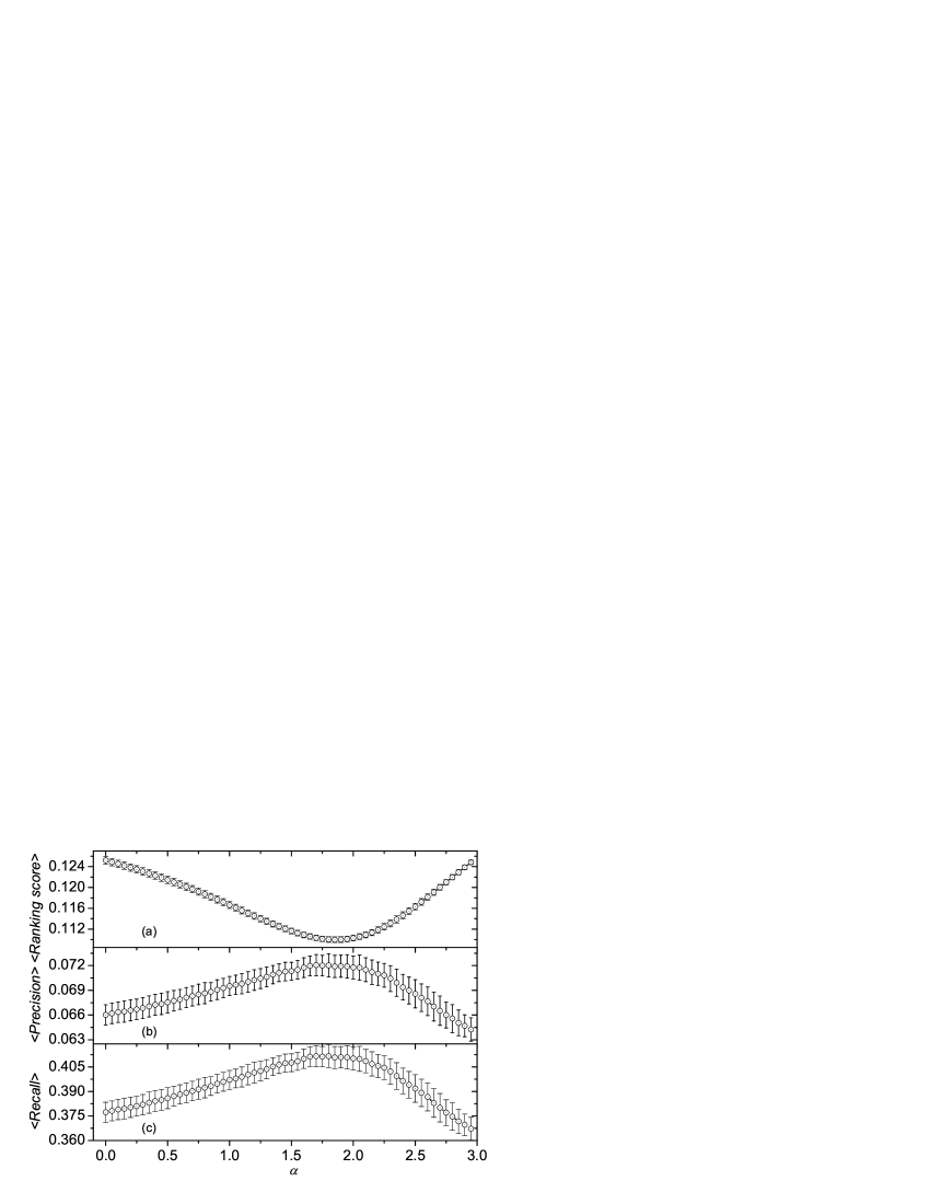
Figure 2: The effect of parameter $\alpha$ in U-MCF. The ranking score has its minimal at about $\alpha$ = 1.85, at almost the same point, the recall and precision achieve their maximums. Present results are obtained by averaging over four independent 90$\%$ vs. 10$\%$ divisions. The error bars denote the standard deviations.

A recommendation algorithm could provide each user a recommendation list which contains all her/his uncollected objects. There are several measures for evaluating the quality of these recommendation lists generated by different algorithms. In this paper, we use ranking score, recall and precision to measure the effectiveness of a given recommendation approach. Good overview of these measures can be found in Ref 5 .

Ranking score. For an arbitrary user $u_{i}$, if the relation $u_{i}$-$o_{j}$ is in the probe set (according to the training set, $o_{j}$ is an uncollected object for $u_{i}$), we measure the position of $o_{j}$ in the ordered queue. For example, if there are 1000 uncollected movies for $u_{i}$, and $o_{j}$ is the 10th from the top, we say the position of $o_{j}$ is the top 10/1000, denoted by $r_{ij}$ = 0.01. Since the probe entries are actually collected by users, a good algorithm is expected to give high recommendations to them, thus leading to small $r$. Therefore, the mean value of the position value $\langle{r}\rangle$ (called ranking score 15 ), averaged over all the entries in the probe, can be used to evaluate the algorithmic accuracy. The smaller the ranking score, the higher the algorithmic accuracy, and vice verse. The definition of ranking score here is slightly different from that of the Ref. 15 . It is because if a movie or user in the probe set has not yet appeared in the training set, we automatically remove it from the probe and the number of total movies was counted only for the ones appeared in the the training set; while the Ref. 15 takes into account those movies only appeared in the probe via assigning zero score to them. This slight difference in implementation does not affect the conclusion.

Recall is defined as the ratio of number of recommended objects appeared in the probe to the total number of objects. The larger recall corresponds to the better performance. Recall is also called hitting rate in literature 15 .

Precision is defined as the ratio of number of recommended objects appeared in the probe to the total number of recommended objects. The larger precision corresponds to the better performance. Recall and precision depend on the length of recommendation list L, we set L as 50 in our numerical experiment (in real e-commerce systems, the length of recommendation list usually ranges from 10 to 100 Schafer2001 ), therefor the total number of recommended objects is $mL$ = 47150.

Fig. 2 reports the algorithmic accuracy of U-MCF, which has a clear optimal case around $\alpha$ = 1.85. Fig. 3 (a) reports the distribution of all the position values, $r_{ij}$, which are sorted from the top position ($r_{ij}$$\rightarrow$0) to the bottom position ($r_{ij}$$\rightarrow$1). Fig. 3 (b) and (c) report the recall and precision for different lengths of recommendation lists respectively. Fig. 4 reports the algorithmic accuracies of the standard case ($\alpha$ = 0) and the the optimal cases ($\alpha$ = 1.85) for different sizes of training sets. All these numerical results strongly demonstrate that to depress the contribution of common selected popular objects can further improve the algorithmic accuracy.

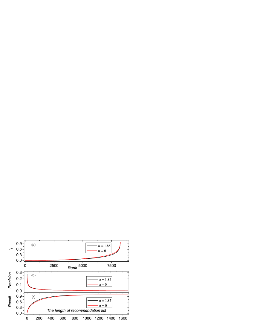
Figure 3: (Color online) (a): The predicted position of each entry in the probe ranked in the ascending order. (b): The precision for different lengths of recommendation lists. (c): The recall for different lengths of recommendation lists.

Figure 4: (color online) The standard CF (SCF) (i.e. $\alpha$ = 0 ) vs. the optimal case for different sizes of training sets.

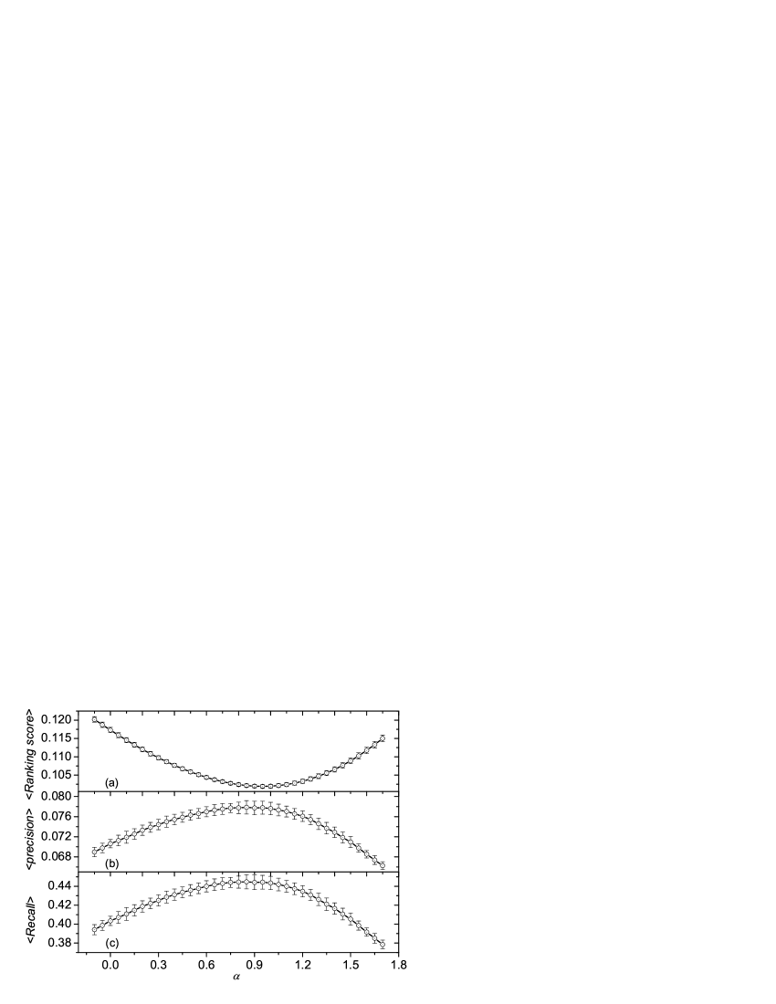
Figure 5: The effect of parameter $\alpha$ in O-MCF. The ranking score has its minimal at about $\alpha$ = 0.95, at almost the same point, the recall and precision achieve their maximums. Present results are obtained by averaging over four independent 90$\%$ vs. 10$\%$ divisions. The error bars denote the standard deviations.

Similar to the U-CF, the recommendation list can also be obtained by object-based collaborative filtering (O-CF), that is to say, the user will be recommended objects similar to the ones he/she preferred in the past Sarwar2001 . By using the cosine expression, the similarity between two objects, $o_{i}$ and $o_{j}$, can be written as:

$$s_{ij}=\frac{1}{\sqrt{k(o_{i})k(o_{j})}}\sum^{m}_{l=1}a_{il}a_{jl}.$$ (7)

The predicted score, to what extent $u_{i}$ likes $o_{j}$, is given as:

$$v_{ij}=\sum^{n}_{l=1,l\neq{i}}s_{jl}a_{li}.$$ (8)

Table 1: Three measures for different algorithms with probe set containing 10$\%$ data. For precision and recall, $L=50$. Present results are obtained by averaging over four independent divisions. The values corresponding to U-MCF and O-MCF are the optimal ones.

method	$<$Ranking score$>$	$<$Precision$>$	$<$Recall$>$
GRM	0.1502	0.3077	0.0540
O-CF	0.1173	0.4035	0.0706
U-CF	0.1252	0.3773	0.0660
O-MCF	0.1019	0.4443	0.0777
U-MCF	0.1101	0.4108	0.0719

Analogously, taking into account the influence of user degree, a modified expression of object-object similarity reads:

$$s_{ij}=\frac{1}{\sqrt{k(o_{i})k(o_{j})}}\sum^{m}_{l=1}\frac{a_{il}a_{jl}}{k^{\alpha}(u_{l})},$$ (9)

where $\alpha$ is a free parameter. The modified object-based collaborative filtering (O-MCF for short) can be obtained by combining Eq. (8) and Eq. (9). Fig. 5 reports the algorithmic accuracy of O-MCF, which has a clear optimal case around $\alpha=0.95$. Fig. 6 (a) reports the distribution of all the position values, $r_{ij}$, which are sorted from the top position ($r_{ij}$$\rightarrow$0) to the bottom position ($r_{ij}$$\rightarrow$1), Fig. 6 (b) and (c) report the recall and precision for different lengths of recommendation lists respectively. Fig. 7 reports the algorithmic accuracies of the standard case ($\alpha$ = 0) and the the optimal case ($\alpha$ = 0.95) for different sizes of training sets. All these results, again, demonstrate that to depress the contribution of users with high degrees to object-object similarity can further improve the algorithmic accuracy of object-based method.

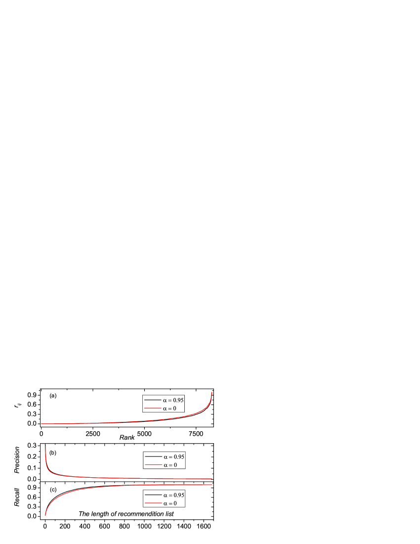
Figure 6: (color online) Similar to Fig.3. But for O-MCF.

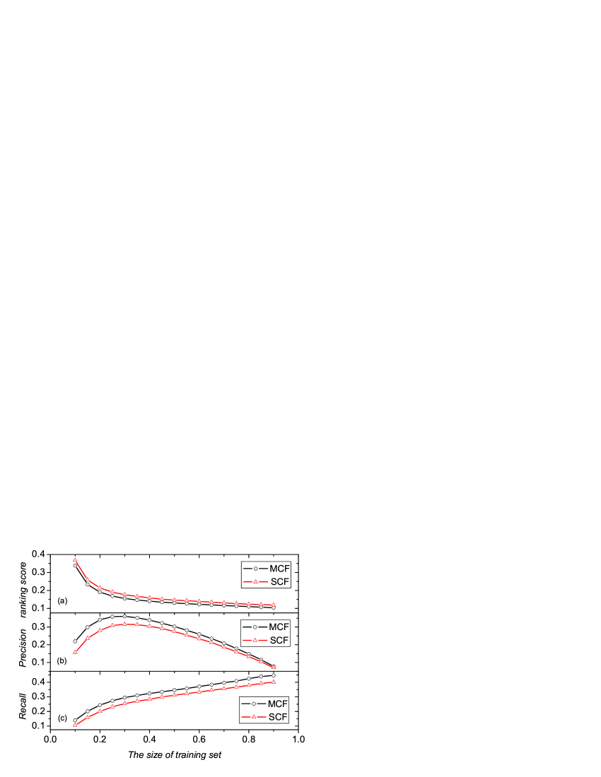
Figure 7: (color online) Similar to Fig.4. But for O-MCF.

IV conclusion

We compare the MCF, standard CF and GRM in Tab. I. Clearly, MCF is the best method and GRM performs worst. Compared with the standard CF, the modified object-based algorithm and the modified user-based method improve the accuracy in different extent in three measures. Ignoring the degree-degree correlation in user-object relations, the algorithmic complexity of U-MCF is $O(m^{2}\langle{k_{u}}\rangle+mn\langle{k_{o}}\rangle)$, the O-MCF is $O(n^{2}\langle{k_{o}}\rangle+mn\langle{k_{u}}\rangle)$, respectively. Here $\langle{k_{u}}\rangle$ and $\langle{k_{o}}\rangle$ denote the average degree of users and objects. Therefore, one can choose either O-MCF or U-MCF according to the specific property of data source. For example, if the user number is much larger than the object number (i.e. $m\gg n$), the O-MCF runs much faster. On the contrary, if $n\gg m$, the U-MCF runs faster. Furthermore, the remarkable improvement of algorithmic accuracy also indicates that our definition of similarity is more reasonable than the traditional one.

References

- (1) M. Faloutsos, P. Faloutsos, and C. Faloutsos, Comput. Commun. Rev. 29, 251 (1999).
- (2) A. Broder, R. Kumar, F. Moghoul, P. Raghavan, S. Rajagopalan, R. Stata, A. Tomkins, J.Wiener, Comput. Netw. 33, 309 (2000).
- (3) G. Adomavicius, and A. Tuzhilin, IEEE Trans. Know. Data Eng. 17, 734 (2005).
- (4) T. Zhou, J. Ren, M. Medo, and Y.-C. Zhang, Phys. Rev. E 76, 046115 (2007).
- (5) J. A. Konstan, B. N. Miller, D. Maltz, J. L. Herlocker, L. R. Gordon, and J. Riedl, Commun. ACM 40, 77 (1997)
- (6) J. L. Herlocker, J. A. Konstan, L. G. Terveen, and J. T. Riedl, ACM Trans. Inform. Syst. 22, 5 (2004).
- (7) M. Balabanovi and Y. Shoham, Commun. ACM 40, 66 (1997).
- (8) M. J. Pazzani, Artif. Intell. Rev. 13, 393 (1999).
- (9) S. Maslov, and Y.-C. Zhang, Phys. Rev. Lett. 87, 248701 (2001).
- (10) J. Ren, T. Zhou, Y.-C. Zhang, Europhys. Lett. 82, 58007 (2008).
- (11) K. Goldberg, T. Roeder, D.Gupta, and C. Perkins, Inform. Ret. 4, 133 (2001).
- (12) T. Zhou, L.-L. Jiang, R.-Q. Su and Y.-C. Zhang, Europhys. Lett. 81, 58004 (2008).
- (13) Y.-C. Zhang, M. Medo, J. Ren, T. Zhou, T. Li, and F. Yang, Europhys. Lett. 80, 68003 (2007).
- (14) J.-G Liu, arXiv:0712.3807.
- (15) Z. Huang, H. Chen, and D. Zeng, ACM Trans. Inform. Syst. 22, 116 (2004).
- (16) P. Holme, F. Liljeros, C. R. Edling, and B. J. Kim, Phys. Rev. E 68, 056107 (2003).
- (17) E. A. Leicht, P. Holme, and M. E. J. Newman, Phys. Rev. E 73, 026120 (2006).
- (18) T. Sorenson, Biol. Skr. 5, 1 (1948).
- (19) The MovieLens data can be downloaded from the website of GroupLens Research (http://www.grouplens.org).
- (20) J. B. Schafer, J. A. Konstan, and J. Riedl, Data Mining and Knowledge Discovery 5, 115 (2001).
- (21) B. Sarwar, G. Karypis, J. Konstan, and J. Riedl, Proc. 10th Int. Conf. WWW, pp. 285-295, 2001.