Longest increasing subsequences, Plancherel-type measure
and the Hecke insertion algorithm
Abstract.
We define and study the Plancherel-Hecke probability measure on Young diagrams; the Hecke algorithm of [Buch-Kresch-Shimozono-Tamvakis-Yong ’06] is interpreted as a polynomial-time exact sampling algorithm for this measure. Using the results of [Thomas-Yong ’07] on jeu de taquin for increasing tableaux, a symmetry property of the Hecke algorithm is proved, in terms of longest strictly increasing/decreasing subsequences of words. This parallels classical theorems of [Schensted ’61] and of [Knuth ’70], respectively, on the Schensted and Robinson-Schensted-Knuth algorithms. We investigate, and conjecture about, the limit typical shape of the measure, in analogy with work of [Vershik-Kerov ’77], [Logan-Shepp ’77] and others on the “longest increasing subsequence problem” for permutations. We also include a related extension of [Aldous-Diaconis ’99] on patience sorting. Together, these results provide a new rationale for the study of increasing tableau combinatorics, distinct from the original algebraic-geometric ones concerning -theoretic Schubert calculus.
1. Introduction and main results
1.1. Overview
Let denote the set of words of length generated using the alphabet . Let denote the length of the longest strictly increasing subsequence of , i.e., the largest with a subsequence such that . Similarly, we consider the length of the longest strictly decreasing subsequence of . Our main goal is to introduce and study a discrete probability measure on Young diagrams, in connection with the study of the distributions of LIS and LDS on uniform random words. An additional goal is to provide a novel motivation for the -theoretic Schubert calculus combinatorics of [BuKrShTaYo06, ThYo07].
There are analogies with the study of LIS and LDS in the permutation case, i.e., when is chosen uniformly at random from the symmetric group . The latter topic has attracted considerable attention; we refer the reader to the surveys [AlDi99, St06] and the references therein. In the permutation case, random Young diagrams are distributed according to the Plancherel measure (on irreducible representations) of . This discrete probability measure is the push-forward of the uniform distribution on , under the Robinson-Schensted correspondence. Schensted [Sc61] established that this correspondence encodes and symmetrically in the shape associated to . In [VeKe77, LoSh77], these ideas are applied to determine the asymptotics of the expectation of over (solving the old “longest increasing sequences problem”), via a study of the “limit typical shape” under the Plancherel measure.
As a continuation of this theme, we apply the Hecke (insertion) algorithm of [BuKrShTaYo06] to define the Young diagram for each ; using this we define Plancherel-Hecke measure. Our belief that this measure should actually be worthy of analysis was initially guided by our theorem that Hecke symmetrically encodes and for , a generalization of Schensted’s theorem. During the course of our investigation, we found that many other aspects of the Plancherel-Hecke measure (conjecturally) also resemble those of the Plancherel measure. This paper records these results, both theoretical and computational, as a justification for further study.
Briefly, this is how the two aforementioned measures compare: Let . Sending , we conjecture that for , our measure is concentrated around the limit typical shape under Plancherel measure. This Plancherel curve plays an important role in [VeKe77, LoSh77]. On the other hand, for we conjecture the measure is concentrated near the “staircase shape”. In particular, a “phase transition” is suggested at . As we tune , a symmetric deformation of the Plancherel curve occurs. In view of the above mentioned result on the Hecke algorithm, this transition phenomenon is further evidenced by computations (with contributions by O. Zeitouni) of the expectation of and as varies; see Section 5 and the Appendix.
There have been earlier extensions of the permutation case to . The limit distribution of the length of the longest weakly increasing/decreasing subsequence (LwIS/LwDS) on was found in work of [TrWi01], following the breakthrough [BaDeJo99] on the limit distribution of on . See also the more recent work [HoLi06]. However, analogous understanding of the distribution of LIS and LDS on appears to be less developed; see, e.g., [Bi01, BoOl07, TrWi01] for contributions.
As a point of comparison and contrast with our approach, previous work on , and utilizes the combinatorics of the Robinson-Schensted-Knuth correspondence, which asymmetrically encodes and . We offer an alternative viewpoint on the relationship between Young diagrams and LIS, LDS. New questions and conjectures are raised, stemming from the Coxeter-theoretic viewpoint of [BuKrShTaYo06] (which in turn generalizes ideas of [EdGr87]).
This text expresses our desire to point out a natural link between the probabilistic combinatorics of LIS, LDS and the combinatorial algebraic geometry of -theoretic Schubert calculus. In particular, we apply and further develop the jeu de taquin for increasing tableaux from [ThYo07], thereby giving another perspective on that work, distinct from the original one. In summary, we believe that the availability of these two disparate interpretations for [BuKrShTaYo06, ThYo07] provides something atypical to recommend -theoretic tableau combinatorics, among the large array of interesting generalizations of the classical Young tableau and symmetric function theories known today.
1.2. Plancherel-Hecke measure
We identify a partition with its Young diagram (in English notation); set . Let denote the set of all Young diagrams. A filling of a shape with a subset of the labels is an increasing tableau if it is strictly increasing in both rows and columns. Let be the set of all increasing tableaux of shape .
We also need set-valued tableaux [Bu02a], which are fillings of assigning to each box a nonempty subset of such that the largest entry of a box is smaller than the smallest entry in the boxes directly to the right of it, and directly below it. We call a set-valued tableau standard if each label is used precisely once. Let denote the set of all standard set-valued tableaux. See Figure 1.
The Plancherel measure on assigns to the probability
Let .
Definition 1.1.
The Plancherel-Hecke probability measure on is defined by letting be a random (non-uniform) Young diagram with distribution
Proposition 1.2.
The Plancherel-Hecke measure is well-defined as a probability distribution; i.e., the following identity holds:
| (1) |
where
| (2) |
There is an exact polynomial-time sampling algorithm
terminating in operations, that induces from the uniform distribution on .
The core technical result of this paper is a generalization of the aforementioned theorem of Schensted [Sc61]:
Theorem 1.3.
Heckeshape simultaneously and symmetrically encodes and as the size of the first row and column of , respectively.
Theorem 1.3 is obtained by establishing another new result, connecting to the “-infusion” operation defined in [ThYo07]. This latter result is an analogue of the classical fact that connects the Robinson-Schensted correspondence to the (ordinary) jeu de taquin rectification procedure.
We prove of Proposition 1.2 in Section 2, after recalling the Hecke algorithm of Buch-Kresch-Shimozono-Tamvakis-Yong [BuKrShTaYo06] (originally constructed to study degeneracy loci of vector bundles). is the Young diagram associated to under . The proof of Theorem 1.3 is given in Section 4.
Example 1.4.
We illustrate the identity (1) for and . There are nine partitions satisfying (2). These are
Then (1) reads
where the products on the righthand side of the equality are listed in order corresponding to the above partitions. Thus, the “typical shape” is , possessing nearly of the distribution. The remainder of the above results will be illustrated in Section 2, after we define Heckeshape.
Theorem 1.3 has some immediate consequences, familiar from the permutation case.
Corollary 1.5.
Under the uniform measure on , we have
| (3) |
In addition,
1.3. Remarks on Proposition 1.2 and Theorem 1.3
In our experiments, Heckeshape was reasonably efficient as a sampling algorithm.111Software available at the authors’ websites. For example, when sampling one Young diagram takes on the order of seconds to minutes on current technology. For larger , we could sample one Young diagram when in several hours on the same technology. A sample when took about one and a half days. The memory demands were modest. In view of the apparent “concentration” suggested below, one sample was enough to be of interest for our purposes, when is large.
There are classical antecedents of Theorem 1.3. As stated earlier, Schensted [Sc61] proved the analogous conclusion about the shape coming from the Robinson-Schensted correspondence for a permutation . In contrast, Knuth [Kn70] proved that the first row of the Robinson-Schensted-Knuth algorithm (RSK) encodes the length of the longest weakly increasing subsequence () of a word .
What is perhaps less well-known is that RSK also encodes as the length of the first column of the shape it associates to . However, unlike Heckeshape, it is asymmetric: is not encoded by the length of the first row (as in general). Thus, the symmetry of Hecke(shape) makes it natural to analyze, as it seems desirable to simultaneously capture the statistics of and .
However, we do not have handy formulas for , or , such as the hook-length formula for . (In the permutation case, the hook-length formula plays a crucial role, see [VeKe77, LoSh77].) In small examples large prime factors appear, showing that such a formula is unlikely. For instance, . This issue is closely related to the open question of finding “good” determinantal expressions for Grothendieck polynomials [LaSc82]. That being said, special cases exhibit connections to work of Stanley [St96] on polygonal dissections, and of [FoGr98] on generalized Littlewood-Richardson rules (further discussion may appear elsewhere). Thus, the enumerative combinatorics of these numbers might of interest in their own right.
It is not difficult to give recursions to calculate and that are useful in moderately large cases. Are there efficient (possibly randomized or approximate) counting algorithms?
Objectively, the lack of simple formulas to compute makes it trickier to apply standard approaches directly; this is an admitted defect of our setting. Nevertheless, we believe the framework of problems described here is tractable. In addition to the results below, in the Appendix one gains useful and nontrivial information about the Plancherel-Hecke measure by exploiting the related work of [Bi01]. In this way, the techniques of [LoSh77, VeKe77] can be applied to the present context.
1.4. Analysis of and the limit typical shape
We organize our analysis by first setting
| (4) |
and considering the limit behavior of when , as . (The case is trivial.) As is explained below, we conjecture that there is a critical value of , denoted : the behavior of is qualitatively different in the intervals and . At , further refinement of the analysis is needed, as we transition from one state to the other.
In the permutation case, to study the Plancherel measure, it is useful to consider the most likely, or “typical” shape. There, three facts are true. First, in the large limit (and after rescaling), a well-defined typical shape exists. Second, the expectation of the LIS and LDS of a large random permutation is encoded respectively in the length of the first row and column of the limit shape. Third, the Plancherel measure is concentrated near the typical shape.
We conjecture that analogues of all three of the aforementioned features also hold for the Plancherel-Hecke measure.
To be more precise, let the typical shape be the shape (contained in ) maximizing . This Young diagram can be interpreted as a step-function. It can furthermore be associated to a piecewise linear approximation . Finally, rescale by
Conjecture 1.6.
-
(I)
For any , there is a unique continuous function
such that for any ,
as . We call this the limit typical shape.
-
(II)
A “phase transition” occurs at :
For , is the line
(5) - (III)
We have reasonable support for the cases (I) and (II) of Conjecture 1.6. Heuristically, part (II) of the conjecture says that when is large, and thus is “close” to , a random word is “close to” being a random permutation. For a permutation, Schensted and Hecke behave the same. Hence the Plancherel and Plancherel-Hecke measures ought to be maximized on the same shape. When is small, the limit typical shape is a rescaling of the “staircase shape” which plays a distinguished role in the Edelman-Greene algorithm [EdGr87] and the Hecke algorithm; see Theorem 1.8 and its proof.
Conjecture 1.6(III) is more speculative, since we did not have as much computational evidence for the shape of . There appears to be a continuous “flattening” of the Plancherel curve to a line as we tune from to . Our data was insufficient to rule out the possibility that is simply a rescaling of the Plancherel curve by a factor of .
Problem 1.7.
Explicitly describe the deformation of when , as varies.
Our best estimate is that (probably just ). However, the values of for relatively small can be experimentally estimated. The table below was based on Monte Carlo estimates of for and and the estimates were stable throughout this range. They closely agree with the conjecture for given above.
| 0.5 | 1 | 2 | 4 | 10 | |
|---|---|---|---|---|---|
| estimate | 0.25 | 0.50 | 0.74 | 0.86 | 0.94 |
Notice that since where is the conjugate shape of we know that if exists and is unique, then is symmetric. This is consistent with the limit curves we predict.
We prove in Section 5 that:
Theorem 1.8.
Conjecture 1.6 is true for . More precisely, in this range, a random shape under satisfies almost surely, as .
The proof of this theorem depends on the analysis of a certain random walk on the symmetric group. Our analysis is not sharp enough to extend to the range , although a refinement might be possible.
Empirically, one finds that the first row and column of are approximations of and that improve as . Therefore, it makes sense to study the asymptotics of and as a means to understand the characteristics of . From this point of view, the following result supports the phase transition phenomena asserted in Conjecture 1.6.
Theorem 1.9 (With O. Zeitouni).
If then , whereas if then . The same statements hold when replaces .
The proof for is a variation on the approach we use to prove Theorem 1.8. We also conjectured the answer for ; after showing O. Zeitouni our guess during an early stage in the project, he communicated to us a proof, and kindly allowed us to reproduce his argument here.
In private communication, E. Rains offered a proof that in the and case. Afterward, in the appendix for this paper, O. Zeitouni and the second author present a simple proof that , for all , in the case, thereby closing the gap in Theorem 1.9. The proof builds on work of [Bi01] (see further discussion in Section 1.5). These results further support the belief that in Conjecture 1.6(III).
In addition, we have the following conjecture about the fluctuation of and .
Conjecture 1.10.
Let denote the standard deviation of . For then
whereas if then
The same statements hold for .
Note that Theorem 1.8 implies Conjecture 1.10 holds for . Tables 3 and 3 give numerical evidence for Conjecture 1.10 and are consistent with Theorem 1.9.
| estimate | 0.45 | 0.50 | 0.55 | 0.60 | 0.75 | 1.00 |
|---|---|---|---|---|---|---|
| 130.00 | 222.50 | 311.06 | 368.38 | 422.48 | 436.36 | |
| 0.00 | 0.63 | 2.86 | 4.01 | 5.07 | 5.09 |
| estimate | 0.45 | 0.50 | 0.55 | 0.60 | 0.75 | 1.00 |
|---|---|---|---|---|---|---|
| 177.00 | 315.43 | 448.2 | 523.63 | 603.78 | 619.64 | |
| 0.00 | 0.67 | 3.52 | 4.62 | 5.90 | 6.29 |
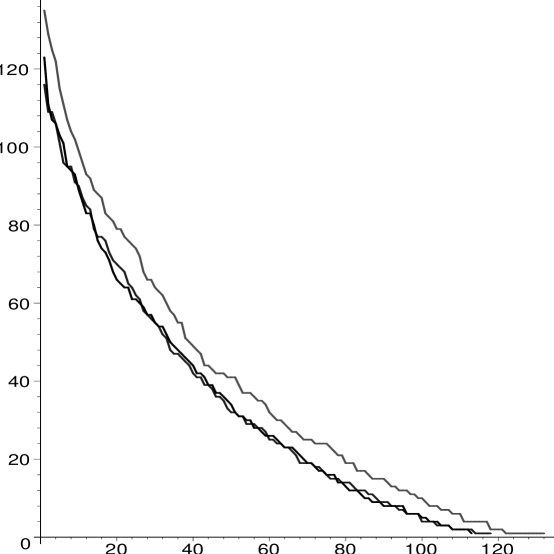
The bulk of appears “concentrated” near , i.e., the probability of sampling a random shape differing, in the sup-norm, from after rescaling, by some fixed , goes to as . See Figure 2: already at we see that two random samples are visibly “close” to one another, and are similar in shape to the third curve which is an approximation of the Plancherel curve. By the curves appear undeniably to be rescalings of one another, with a rescaling factor of about in our experiments. Naturally, as gets larger, the empirical convergence of the curves occurs faster.
1.5. Further comparisons with the literature
As mentioned earlier, the limit distribution of on permutations, and that of on words is well understood.
The study of LIS on was considered, e.g., in [TrWi01]. In addition, the study of the distribution of LIS, in the critical case is implicit in [Bi01, BoOl07]. In [Bi01], an alternative measure on Young diagrams is studied: Schur-Weyl duality implies that one has the decomposition
where here is the irreducible Specht module and is the irreducible Schur module. Now taking dimensions one defines a probability measure that assigns to the likelihood . Biane explicitly determines the rescaled limit typical shape in this context. Combinatorially, Biane’s measure arises from the RSK algorithm. Since we know that encodes the in the first column (by reading backwards), one expects, by analogy with [LoSh77, VeKe77] that a certain rescaling of the first column of Biane’s limit shape is the of Conjecture 1.6. However, to justify this conclusion rigorously one needs more work. Further, the fluctuations around Biane’s curve have been studied, in the case, by Borodin-Olshanski [BoOl07].
Hecke was originally developed in [BuKrShTaYo06] as a generalization of the Edelman-Greene correspondence which bijects Coxeter reduced words in the symmetric group to pairs of tableaux [EdGr87]. Our proof of Theorem 1.3 implies that this algorithm encodes the LIS of such words, although the study of LIS of reduced words appears unmotivated. On the other hand, the Coxeter-theoretic viewpoint on words will be useful in our analysis of LIS, LDS and .
1.6. Summary and organization
In Section 2 we recall the Hecke algorithm and give an additional example of the results of Section 1.2. We then prove Proposition 1.2. In Section 3, we include two consequences of Theorem 1.3. We split our remaining proofs according to the main flavor of technique used: in Section 4 we explain the increasing tableau theory we need from [ThYo07] and prove Theorem 1.3. In Section 5, we utilize probabilistic-combinatorial techniques, combined with our main results, to prove Theorems 1.8 and 1.9.
2. The Hecke algorithm
2.1. The -Hecke monoid
We need to recall some notions used in [BuKrShTaYo06]. The -Hecke monoid is the quotient of the free monoid of all finite words in the alphabet by the relations
| (7) | for all | |||||
| (8) | for all | |||||
| (9) | for . |
There is a bijection between and the symmetric group . Given any word there is a unique permutation such that for any reduced word of ; see, e.g., the textbook [BjBr05] for basic Coxeter theory for the symmetric group. In this case, we write and say that is a Hecke word for . Indeed, the reduced words for are precisely the Hecke words for that are of the minimum length , the Coxeter length of (after identifying the label with the simple reflection ). Given an additional permutation with Hecke word , the Hecke product of and is defined as the permutation .
The (row reading) word of a tableau , denoted , is obtained by reading the rows of the tableau from left to right, starting with the bottom row, followed by the row above it, etc. We also define . So for example, if is the increasing tableau of Figure 1, then .
The Hecke algorithm defined in [BuKrShTaYo06] identifies pairs of words
where is a Hecke word and satisfies
with pairs of tableaux of the same shape, where is an increasing tableau such that and the content (i.e., multiset of labels) of matches the content of . We refer to the -tableau as the insertion tableau and the -tableau as the recording tableau. (We point out that the “column” convention in [BuKrShTaYo06] differs slightly from the “row” one used here.)
2.2. Description of Hecke and Heckeshape
The following description of Hecke was originally given in [BuKrShTaYo06]:
Description of Hecke: In this algorithm, one inserts an integer into an increasing tableau . We denote this by . The output is a triple where is a modification of (possibly ), is a corner of and is a parameter. Initially, we attempt to insert into the first row of , and an output integer is possibly created which is inserted into the next row and so on, until no output integer is created. We refer to this final insertion as the terminating step, and the previous insertions as bumping steps.
Suppose is a row that we are attempting to insert into. If is larger than or equal to all the entries of , then no output integer is generated and the algorithm terminates: if adjoining to the end of results in an increasing tableau , then set and to be the new corner added. Otherwise end with the present , without modification; and is the corner that is at the end of the column containing the rightmost box of . On the other hand, if contains boxes strictly larger than , let be the smallest such box. If replacing with results in an increasing tableau, then do so. In either case, is the output integer to be inserted into the next row.
Inserting a word using this algorithm terminates with an increasing tableau
The tableau is obtained by placing each in the -corner resulting from the insertion of .∎
We also have the following reverse insertion algorithm .
Description of : Let be an increasing tableau, a corner of , and . Reverse insertion applied to the triple produces a pair of an increasing tableau and a positive integer as follows. Let be the integer in the cell of . If , remove . In any case, reverse insert into the row above the corner .
Whenever a value is reverse inserted into a row , let be the largest entry of such that . If replacing with results in an increasing tableau, then this is done. In any case, the integer is passed up. If is not the top row, this means that is reverse inserted into the row above of ; otherwise becomes the final output value, along with the modified tableau.
We now complete the description of . Locate the bottom-most corner with the largest label, in the tableau, and remove the label. If it was the only entry in its corner, remove the corner, set . Otherwise set . Set to be this corner. Then reverse insert . Repeat until all the entries of (and ) have been removed. ∎
Hecke is a generalization of the Robinson-Schensted correspondence in the sense that it agrees with that correspondence whenever is a permutation in . In that case the and tableaux are both standard Young tableaux.
In this paper, we are only concerned with the case . Therefore, we also set and define
by setting to be the common shape of and under . (An alternative description of this map is given in Theorem 4.2 in Section 4.)
Example 2.1.
Let . Then the reader can check that Hecke produces the following steps:
Here and indeed the length of the first row of this shape equals , whereas the length of the first column equals .
2.3. Proof of Proposition 1.2
The claim that is a probability distribution follows if Hecke extends to provide a bijection between:
where satisfies (2).
Associate to each word the pair . Clearly injectively maps these pairs into .
To prove surjectivity, let . Then under , corresponds to some pair . Now since that is the only possible sequence that can arise from a standard tableau . Also, since , must use some subset of . Thus . Hence . The claim (2) is then clear from the properties of Hecke.
Finally, from the above discussion it is immediate that Heckeshape is a sampling algorithm for . The bottleneck of the algorithm is the insertion process (a random uniform word can be generated in time). By (2) we know that each of the insertions demand at most operations. Hence operations are needed. This completes the proof of Proposition 1.2.∎
3. Some further consequences of Theorem 1.3
3.1. A generalization of the Erdős-Szekeres theorem
The following classic result is due to Erdős-Szekeres [ErSz35]:
Theorem 3.1.
Let . If then or .
It is known that this result can be readily deduced from Schensted’s results, see, e.g., [St06, Section 2]. Theorem 1.3 similarly leads to an extension of Theorem 3.1 that relates LIS and LDS to Coxeter length.
Proposition 3.2.
Let . Suppose and
| (10) |
then or ; recall is the permutation identified with .
Proof.
Example 3.3.
If and then if then or . This inequality is tight in the sense that the bound cannot be reduced: consider . This is already a reduced word of Coxeter length , viewed as an element of , and .
3.2. Patience sorting for decks with repeated values
In [AlDi99], the Schensted correspondence was connected to the one-person (solitaire) card game patience sorting. We include a generalization of this connection, which in particular is a refinement of the LIS claim of Theorem 1.3.
In this game, a deck of cards labeled is shuffled and the cards are turned up one at a time and dealt into piles on the table: a lower card may be placed on top of a higher card, or put into a new pile to the right of the existing piles. The goal of the game is to finish with as few piles as possible.
For example, if and the deck is shuffled in the order
then the top card is dealt onto the table. The can either be placed to the right of the or on top of it – suppose we chose the latter scenario. Next the must be placed to the right of the pile containing the and , starting a new pile. At this stage, we have .
The greedy strategy is to always place the new card in the leftmost pile possible. If we complete the game using this strategy, we would obtain, successively:
It is easy to prove that the top cards increase from left to right throughout the game; Mallows [Ma73] and later independently Hammersley [Ham72, p. 362] observed that the number of piles at the end equals , where is the permutation defining the shuffled deck. Finally, Aldous-Diaconis note that the first row of the insertion tableau under Robinson-Schensted agrees with the top cards.
Aldous-Diaconis [AlDi99, Section 2.4]) consider two variants of patience sorting where the deck has repeated entries, i.e., where all cards of the same rank (e.g., all Jacks) are equal. The two rules they consider are “ties forbidden” and “ties allowed”, depending on whether or not a Jack can be placed on top of another Jack. They provide an analysis of the former case, relating it to the Robinson-Schensted-Knuth correspondence.
For example, if the shuffled deck is given by , then the result of playing patience (using the greedy strategy) with ties forbidden and allowed, respectively, are:
Proposition 3.4.
Assume patience sorting is played with ties allowed, on a deck of cards with distinct types of cards (viewed as a word ). Then
-
(I)
The top cards of each pile at the termination of the game, using the greedy strategy, as read from left to right, agree with the top row of the insertion tableau of .
-
(II)
The optimal strategy (minimizing the number of piles created) is the greedy strategy, and piles are created.
Proof.
The proof of (I) is an easy induction, comparing the description of Hecke with the “tied allowed” rules of patience sorting.
Briefly, probabilistic and statistical analysis on the “tied allowed” case of patience sorting is possible, in analogy to the work of [AlDi99]. Below we have tabulated the results of a Monte Carlo simulation with trials on a standard -card deck. Typically, the number of piles is between and . The average number of piles is which, naturally, is less than the average number of piles when the deck is totally ordered, which is as reported by Aldous-Diaconis. So a deck ordering is “lucky” if the number of piles is less than , which occurs only about of the time.
| number of piles | 6 | 7 | 8 | 9 | 10 | 11 | 12 | 13 |
|---|---|---|---|---|---|---|---|---|
| frequency | 82 | 2993 | 20336 | 39039 | 27843 | 8489 | 1166 | 52 |
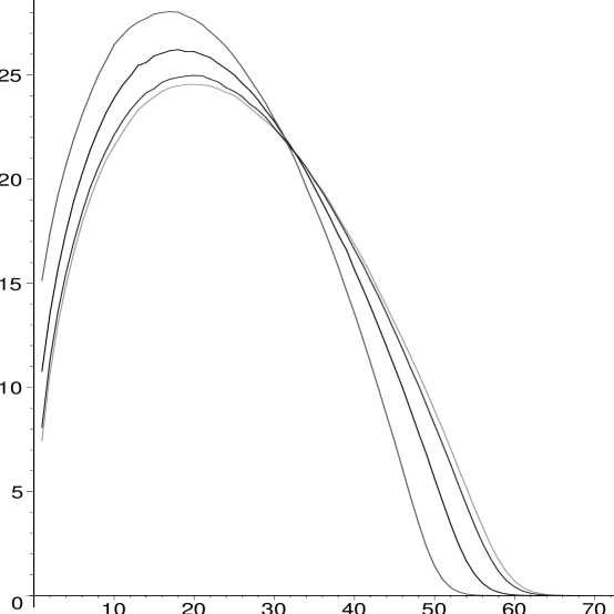
Figure 3 shows that there is a definite shape describing the mean pile sizes as varies. Questions about the structure of this shape may be interpreted as enriched questions related to LIS. One can analyze such questions using the dichotomy of Section 1.4; we do not pursue this here.
4. Increasing tableau theory and the proof of Theorem 1.3
Now we show that the size of the first row of computes . Let be the largest index such that the longest strictly increasing subsequence ending at has length . For example, if then , and . We now in fact prove the following claim, which is stronger than the LIS assertion of Theorem 1.3 (cf. [St99, Prop. 7.23.10]):
Proposition 4.1.
Suppose , and is the insertion tableau of . Then the first row of is given by .
Proof.
By induction on . The base case is trivial.
Suppose that the claim holds for . Thus if is the insertion tableau of then by induction, the first row is given by
where .
We consider the possibilities of what happens as we insert into the first row of . We prove the desired conclusion holds for the case that for some maximally chosen ; other cases are similar. So after inserting , the first row of is
The assumption shows that the longest increasing subsequence in using is of length at least , since we can adjoin to the length subsequence ending at . On the other hand, is of length at most since if it were, say, of length , there must be a length increasing subsequence in ending at with and . But this is a contradiction of the definition of since we would then have a length increasing subsequence ending at .
Since we have just shown , it is now clear that for . Thus, the first row of satisfies the desired claim, and the induction follows. ∎
In order to prove that the first column of computes , we need to draw a connection to [ThYo07], where we developed a -theoretic jeu de taquin theory. Rather than repeat the setup in full here, for brevity, we refer the reader to that paper for the complete background on -rectification and -infusion used below.
Although what follows also constitutes a proof of our LIS claims, we felt that including the direct proof via the stronger claim of Proposition 4.1 was worthwhile. However, a similarly direct proof of our LDS claim seems harder.
Let
be the staircase shape. Also, let be the permutation shape consisting of single boxes arranged along an antidiagonal. Given , define to be the tableau where is arranged from southwest to northeast. Also let be the superstandard Young tableau, i.e., the one whose first row is labeled , the second row is labeled by etc. This latter tableau determines a particular -rectification of , which by definition is -, see [ThYo07, Section 3]. (An important subtlety in -theoretic jeu de taquin is that -rectification depends on the order in which it is performed, unlike the rectification of classical jeu de taquin. However, the order defined by is particularly nice.)
The following result is an analogue of a classical result linking the Robinson-Schensted algorithm to the (ordinary) rectification of :
Theorem 4.2.
Let . Then - is the insertion tableau of .
Proof.
We induct on . The base cases are easy. We may assume that the steps of the that are defined by the “inner” labels results in a skew shape of the form , as depicted below:
| (11) |
The induction hypothesis is that is the insertion tableau obtained by Hecke inserting . (In the depiction of from (11), some of the boxes with labels may be empty.) The non-underlined labels occupy the boxes of , whereas the underlined labels dictate the remaining steps to perform to complete the - computation (these steps are recalled below).
Hence it remains to show that the tableau obtained by the Hecke-insertion is the same as carrying out the - indicated by (11), i.e., the operation
| (12) |
To do this, we first develop a technical fact. In [ThYo07, Section 1.1], we defined the procedure switch, which we restate now (in a more convenient form). Let be the set of mixed tableaux, which, by definition, are tableaux of shape , each of whose boxes is filled with an entry from one of two alphabets, and , such that, within each row or column, the entries for each alphabet appear at most once. (No increasingness condition is demanded.) We also include the null tableau , as a special element of .
Define an operator
as follows. Given , consider the subshape of consisting of boxes whose entry is either or . For each non-singleton connected component of , interchange the ’s and the ’s. If this results in a (non null) mixed tableau, then the result is that tableau. Otherwise the result is . By definition .
Example 4.3.
Let and . Then is given below, together with two different switch computations applied to it:
On the other hand,
The following lemma is easy to verify from the definitions:
Lemma 4.4.
If and then the operators and commute, i.e.,
is a relation in the algebra generated by switch operators on .
The procedure described in [ThYo07, Section 3] for computing - is to consider the entries of as being underlined, where the maximum entry of is , say, and the entries of as not underlined, where the maximum entry of is . Now perform the following sequence of operations, from left to right, as indexed by:
| (13) |
We refer to this sequence of pairs (interchangeably, the corresponding sequence of switch operators) as the standard switch sequence.
The technical fact we need is that - can in fact be computed differently: a switch sequence is called viable if it is a “shuffling” of (13), in the following sense:
-
•
every occurs exactly once, for and ;
-
•
for any , the pairs occur in that relative order; and
-
•
for any the pairs occur in that relative order.
This definition is explained by the proof of the following proposition:
Proposition 4.5.
Any viable switch sequence can be used to calculate -infusion.
Proof.
Thus, in view of Proposition 4.5, to complete the induction it suffices to construct a viable switch sequence whose result is the same as . (A caution: in [ThYo07] it was shown that the standard switch sequence necessarily maintains increasingness along rows and columns of the members of each alphabet. We will not prove that a viable switch sequence also achieves this during the intermediate steps of a -infusion. However, this does not play a logical role in how we apply Proposition 4.5 below.)
Let , and for , let be the number which is inserted in row according to Hecke insertion of into . During a bumping step of Hecke insertion, let be the smallest number already in row which is greater that .
We say that a mixed tableau, obtained after some number of switch operations applied to , is in row normal form if:
-
•
the -th row is of the form
where has not yet moved from its initial position in column , or
depending, respectively, on whether the Hecke insertion terminates at row or after, or strictly earlier. Here the -th row of has length ; and
-
•
all non-underlined symbols in rows and below have not moved from their initial positions.
Having explained our general strategy, what remains is some tedious but straightforward case analysis to describe the viable switch sequence we use: Our initial mixed tableau is in row normal form. Now, suppose we have arrived, after some sequence of applications of (A), (B) and (C) below, at a mixed tableau in row normal form. There are three possibilities for a bumping step of Hecke insertion of .
(A) is inserted, bumping : Consider the switch sequence that moves to the left along row : specifically, using
| (14) |
until it is directly above the in row , and then, starting from the right, swaps each box in row having an underlined label with the one directly below, which has a non-underlined label (this can always be done since no label numerically equal to appears among the latter boxes, by assumption). The result is therefore in row normal form since doesn’t move in this process, it is the unique box with a non-underlined label in row , and , as demanded.
Note that the non-underlined labels of the -th row of the mixed tableau we obtain after this process is the same as the -th row of , with replaced by , as desired.
Example 4.6.
If and we started with
|
|
so that and , then we begin by moving above :
|
|
We conclude with , and then finally , resulting in
which is in row () normal form. Moreover, the non-underlined labels in row of this mixed tableau, namely agrees with the first row of , as desired.
(B) is not inserted because of a horizontal violation: (That is, a label numerically equal to already appears in the row that we are Hecke inserting into.) Proceed as in (A) by moving to the left, until it is directly above , i.e., apply (14). Now, “locally” the situation in the column containing and the column to its left is:
for some . The former case shows rows and when does not appear in row , while the latter case also includes row if it does. To the right of the column containing , we swap boxes with underlined and non-underlined labels, as in (A). Then we perform the transformation
| (15) |
respectively. After this transformation, we complete by swapping, right to left, the boxes to the left of the , as in (A). The result is in the demanded row normal form.
Note that unlike (A), row still has a box with an underlined label in it. However, when we work on the row normal form, the reader can check that our descriptions will force that box to be filled by : e.g., if we apply case (A) next, this will occur when we execute the switches (14), if we apply case (B) next, this will occur when we execute either the switches (14) or (15), whereas if we apply (C) next, the replacement will occur during the switches (16) below. Hence, in the end, we find that the non-underlined labels in row are the same as the -th row of the Hecke insertion of into , as desired.
Example 4.7.
If and we started with
|
|
then moving the “” in row to the left, as in (A), gives
The remaining swaps give
and the latter is in row normal form. The mild complication of this case, as suggested above, is that row is not yet the same as the first row of the insertion tableau of Hecke.
However, as we begin to work on this row normal form, we start by using (beginning to move the in row to the left), giving:
Hence row now does agree with Hecke insertion.
(C) will not be inserted because of a vertical violation (and a horizontal violation does not occur): While Hecke inserting into row of , is directly below a label (numerically equal to) that is in row . This prevents one from replacing by the we are inserting. (Note that this case can only occur if .) Moreover, since there is no horizontal violation, the number immediately to the left of , say , satisfies . Notice, in order for a vertical violation to occur, the previous step of Hecke inserting must have been an instance of case (B) or (C) (since we are Hecke inserting a number into row which also appears in row ). Hence the box directly above and to the left of the contains an underlined label .
Now we begin by switching all the boxes with underlined labels in row to the right of , with the non-underlined labels directly below them. The remaining switches, which involve the rows to , in the column of and the column to its immediate left, are as given as follows:
| (16) |
As in (B), we finish by completing a sequence of swaps involving the columns to the left of the . The result of this process is a tableau in row normal form.
As at the conclusion of (B), row of the resulting row normal form mixed tableau, still contains an underlined label. As in that case, this label will be switched with , as desired, during the forthcoming switches.
Example 4.8.
To give an example of (C), the previous insertion must have been of type (B) or (C), so consider the following example:
After the first step, an insertion of type (B), we reach row 2 normal form:
As compelled by the conditions of a viable switch sequence, we switch with before we switch with 5, and as a result, as described above, we get to row 3 normal form:
The final result is:
Again, this tableau agrees with .
Note that after each of (A), (B) and (C), when we reach row normal form, is necessarily in a column weakly to the left of , because is an increasing tableau and together with the rows strictly below row are, at this point, still unaltered. This observation guarantees that the switches as described above can actually be executed, i.e., the above descriptions are well-defined.
Using similar analysis one can give switch sequences for the terminating steps of Hecke insertion, such that one maintains row normal form for all , where is the number of rows of . We leave the straightforward details to the reader.
These constructions then show, by induction on the number of rows , that we have a sequence of switch operations transforming into .
Conclusion of the proof of Theorem 4.2: by the fact that is an increasing tableau, and by the definition of normal form, it is easy to see that the sequence of operations used forms a viable sequence, after suitable insertions of any trivial operators (that is to say, switch operations which do not have any effect on the tableau). We can therefore apply Proposition 4.5 as we claimed earlier. ∎
Example 4.9.
Continuing Example 4.8, the switch sequence we obtain, by following the descriptions of the cases (B) and (C) that are needed is:
This is not quite a viable sequence: although our constructions guarantee that it satisfies the second and third conditions to be a viable sequence, it fails the first, since, e.g., doesn’t appear in the sequence, since this switch is never needed. However, clearly we can simply insert this trivial switch, along with the others that are missing, giving the viable sequence:
The action of this viable sequence on the original mixed tableau is therefore the same as the original switch sequence, which we highlight in boldface. This viable sequence also happens to be the standard switch sequence, although it needn’t be in general. Hence
in agreement with Theorem 4.2.
In [ThYo07, Theorem 6.1] we showed that the first row of - has length , for any increasing tableau of shape . So by Theorem 4.2, the first row of has length . By symmetry, [ThYo07, Theorem 6.1] also implies that the first column of - has length . Hence the LDS claim follows. This completes the proof of Theorem 1.3. ∎
Given , define . The following is symmetry statement is immediate from Theorem 1.9, since :
Corollary 4.10.
Let and . Then and where and are the conjugate shapes of and respectively.
A warning is needed: unlike Robinson-Schensted correspondence setting, with Hecke, one cannot conclude that the insertion tableaux associated to and differ only by a reflection across the main diagonal. A counterexample is . (In [Sc61], the symmetry property of the Robinson-Schensted correspondence, was applied to prove the LDS claim in the classical version of Theorem 1.3.)
Problem 4.11.
Give an explicit description of in terms of .
Finally, Greene [Gr74] has given an explanation of the other rows of the shape associated to a permutation under the Robinson-Schensted correspondence: equals the maximal size of a union of disjoint increasing subsequences of .
However, we could not find any extension of Greene’s theorem in the Hecke context. The naive tries do not work: Since , the simplest case to analyze is when . The example corresponds to ; this shows that it is not valid to merely replace “increasing” by “strictly increasing” in Greene’s theorem, since that would predict .
5. Probabilistic combinatorics and proofs of Theorems 1.8 and 1.9
Proof of Theorem 1.8: Let be the word in of maximal Coxeter length. Hence . This is the unique permutation in with this length.
We need the following lemma, which characterizes when is maximized.
Lemma 5.1.
For , if and only if .
Proof.
First suppose . Under , the insertion tableau satisfies . Hence the shape of has at least boxes and so by Proposition 1.2 it must be .
Conversely, if , then note that there is a unique increasing filling of that shape (using in the first row, in the second row, etc). Then it is well-known that . ∎
In view of the Lemma 5.1, the Theorem will follow if we can show that
| (17) |
(We conjecture this to be true whenever . This would imply Conjecture 1.6 for this entire range.)
Set . Then either
depending on whether the simple reflection (say equal to ) is an ascent of or not. (An ascent occurs at a position for a permutation if .)
Provided that , has at least one ascent. Thus when , the probability that ’s introduction increases the Coxeter length is at least .
Let
Related to this, let be Bernoulli distributed with parameter . Set
Clearly,
| (18) |
We now show that when
the righthand side of the inequality (18) goes to zero as .
This is a simple application of (a special case of) Bennet’s large deviation inequality, see, e.g., [DeZe02, Cor. 2.4.7]: suppose are independent, mean zero random variables with . Set . Then for we have
| (19) |
To apply this to our setting, let . Hence . Then with
The result then follows. ∎
In the above argument, we interpreted as a random walk in that begins at the identity and works its way up in the weak Bruhat order to . At each step the probability of going up is at least (as we have used), but is larger in general. However, since this probability varies, even for permutations with the same Coxeter length, a more refined analysis is needed to push the argument we have used further, up towards .
Given let
Let and set
Provided occurs, then
with probability , and is equal to otherwise.
Let and be discrete random variables, where is Bernoulli distributed with parameter . Now,
Thus it will be enough to show that when then
This is another application of the large deviation inequality (19).
For we use a proof provided for us by O. Zeitouni: , the expected length of the longest weakly increasing subsequence of (with ) is known to satisfy
see [Joh01, Theorem 1.7]. The argument shows that the difference between the LIS and LwIS of is typically small.
Let be the random variable for the value of of a random uniform word where is the integer part of , etc. Similarly define where replaces .
Fix and let be large enough such that
| (20) |
We need a “graphical” representation of a word in : consider a rectangle subdivided into unit squares. In each of the columns, one places a single “dot” in one of the rows. The set of such configurations is in obvious bijection with words in .
Given , draw smaller rectangles of dimension along an antidiagonal inside the rectangle, as depicted in Figure 4 below.
Label the -th southwest most box . Let be the random variable giving the number of dots in . Notice that the ’s are independent. Also, the dots inside define a word, and we can speak of and , the length of the longest strictly (respectively, weakly) increasing subsequence of that word.
Say that is good if the following conditions simultaneously hold:
-
(a)
;
-
(b)
; and
-
(c)
no two dots in have the same height (hence ).
Now, we have
and we claim for an sufficiently large, for , and for all large, we have:
The proof is a standard argument: let be the indicator random variable which evaluates to if column has a dot that lies in the box that occupies that column (hence with probability ), and evaluates to otherwise. Hence
where the previous line is an application of Chebyshev’s inequality. Now take sufficiently large (bigger than some ) so .
Assuming , if the event (a) occurs, then with probability at least , when is large, (b) holds, because of the definition of using (20).
The probability of the event (c) not occurring is bounded above (using a union bound) by
because .
So,
for and large.
Another standard argument with Chebyshev’s inequality shows with high probability, say at least , and for large, the number of good boxes is
Hence, with that probability, for
Since
the case follows by taking , completing the proof of the theorem. ∎
6. Appendix (by A. Yong and O. Zeitouni)
The goal of this appendix is to present a proof of the following result:
Theorem 6.1.
Let . Then
where
However, in order to prove this statement, we need to work with another variant of Plancherel measure, utilized, e.g., by [Bi01] and alluded to in Section 1.5 of the main text. Our approach parallels the one developed in [LoSh77, VeKe77] to prove in the permutation case, by utilizing work of [Bi01].
6.1. Preliminaries
A semistandard Young tableau of shape with labels from is a filling of the Young shape with these labels so that the entries weakly increase along rows, and strictly increase along columns. For example, if and there are two such tableaux: and . Let denote the number of such tableaux.
Define the Plancherel-RSK measure on the set of Young diagrams with boxes, by declaring that a random Young shape occurs with probability
We make no claims of originality in this definition. Indeed, this is the same measure studied in, e.g., [Bi01]; although there the measure is defined in terms of dimensions of irreducible and modules associated to ; the equivalence is well-known. The fact that is in fact a probability distribution follows from either Schur-Weyl duality, as in Section 1.5, or by the RSK algorithm, see, e.g.,[St99, Section 7.11].
A crucial advantage of for the purposes of understanding , in comparison to Plancherel-Hecke measure, is that both and have simple multiplicative formulas. This makes it more readily analyzed using ideas of [LoSh77, VeKe77], which we modify to the present setting.
Given a box , define the hook-length associated to to be where is the number of boxes strictly to the right of , and in the same row, and is the number of cells strictly below and in the same column. Then we have [St99, Chapter 7], the hook-length formula and hook-content formulas, respectively:
where in the second formula is the content of , the column index of minus the row index of . So for example, if , the contents are given by
6.2. Plancherel-RSK as a Markov measure
Young’s lattice is the poset structure on where if the shape of is contained in the shape of . We write to denote a covering relation in this poset, i.e., where is obtained from by adding a single box at a corner.
Define a Markov process on with the transition probabilities
We need the following lemma, that in particular shows that Plancherel-RSK measure is a Markov measure with the above transition probabilities.
Lemma 6.2.
-
(I)
-
(II)
Proof.
The claim (I) is equivalent to
This follows from the following Pieri rule for Schur polynomials
See [St99, Theorem 7.15.7]. Here
is the Schur polynomial, where the sum is over all semistandard Young tableaux of shape with entries from , , and is the number ’s used in . In particular, (I) is immediate from .
For (II), the claim is
that is, , which is well-known (and straightforward from the definitions). ∎
6.3. Conclusion of Proof of Theorem 6.1
Work of Biane [Bi01, Theorem 3] describes the typical shape under Plancherel-RSK after the rescaling . Biane’s theorem implies that
| (21) |
but not
| (22) |
Briefly, we explicate how his work applies to our situation (the reader is directed to the original source for details): Biane works with the coordinate axes rotated -degrees counterclockwise, as in, e.g., [VeKe77, VeKe85]. His aforementioned theorem states that if is any sequence of (rescaled and rotated) Young diagrams, then for any we have
| (23) |
where the probability is computed with respect to . Also, is Biane’s limit shape, which has the property that it meets the line at a distance from the origin. In other words, the “first column” of satisfies
| (24) |
For each , let be the length of the first column of . From (23) it follows that for any ,
| (25) |
Moreover, since it is known that for any the first column of the Young diagram associated to equals , (21) follows immediately from (24) and (25) combined.
Note that the above argument does not also prove (22) since (23) does not rule out the possibility that consists of Young diagrams with “tails” along the axis that both “lengthen” and “thin out” as . Therefore, it remains to verify (22).
To do this, we modify an argument found in [VeKe85], which establishes the analogous assertion in the permutation case: consider the set of all sequences of Young diagrams
where for .
For a Young diagram , let denote the diagram obtained by adding a single box to , in the first column. For each integer , define the indicator function by setting if , and setting otherwise.
Studying the expectation of we have:
where we have just used
Let
Note that by the hook-content formula we have
where is the length of the first column of .
Summarizing, we have
| (26) |
where denotes the expectation of , i.e., the expected length of the first column of a random shape with boxes, drawn under the Plancherel-RSK measure.
Notice also that since is an indicator random variable, we have
| (27) |
Therefore, combining (26) and (27) we obtain, by the Cauchy-Schwarz inequality, the following difference inequality:
| (28) |
We claim that .
To prove this, note the following facts about :
-
(a)
; and
-
(b)
.
Now define a linear interpolation: for , set
| (29) |
Note that for such , . Therefore, combining equations (28) and (29) we obtain
| (30) |
Since we have , hence the above differential inequality is equivalent to
Hence it follows that
That is,
Now we care about . We always have (trivially), but for we have the better inequality . Therefore,
for and
for . The result then follows.∎
Acknowledgments
HT was supported by an NSERC Discovery Grant. AY was supported by NSF grant DMS 0601010 and a U. Minnesota DTC grant during the Spring 2007; he also utilized the resources of the Fields Institute, and of Algorithmics Incorporated, in Toronto, while a visitor. We would like to thank Ofer Zeitouni for allowing us to include his proof for the case of Theorem 1.9 and for his extensive help during this project. We also thank Alexander Barvinok, Nantel Bergeron, Alexei Borodin, Sergey Fomin, Christian Houdré, Nicolas Lanchier, Igor Pak, Eric Rains, Mark Shimozono, Richard Stanley, Dennis Stanton, Craig Tracy and Alexander Woo for helpful correspondence.
References
- [AlDi99] D. Aldous and P. Diaconis, Longest increasing subsequences: from patience sorting to the Baik-Deift-Johansson theorem, Bull. Amer. Math. Soc. 36(1999), 413–432.
- [BaDeJo99] J. Baik, P. Deift and K. Johansson, On the Distribution of the Length of the Longest Increasing Subsequence of Random Permutations, J. Amer. Math. Soc., 12(1999), 1119–1178.
- [Bi01] P. Biane, Approximate factorization and concentration for characters of symmetric groups, Inter. Math. Res. Notices 2001(2001), no. 4, 179–192.
- [BjBr05] A. Björner and F. Brenti, Combinatorics of Coxeter Groups, Graduate Texts in Mathematics 231, Springer, New York, 2005.
- [BoOkOl00] A. Borodin, A. Okounkov and G. Olshanski, Asymptotics of Plancherel measures for symmetric groups, J. Amer. Math. Soc., 13(2000), 481–515.
- [BoOl07] A. Borodin and G. Olshanski, Asymptotics of Plancherel-type random partitions, J. Algebra 313(2007), 40–60.
- [Bu02a] A. Buch, A Littlewood-Richardson rule for the -theory of Grassmannians, Acta Math., 189 (2002), 37–78.
- [BuKrShTaYo06] A. Buch, A. Kresch, M. Shimozono, H. Tamvakis and A. Yong, Stable Grothendieck polynomials and -theoretic factor sequences, Math. Ann., to appear, 2008. math.CO/0601514.
- [DeZe02] A. Dembo and O. Zeitouni, Large deviations and applications, Handbook of stochastic analysis and applications, 351–416, Statist. Textbooks Monogr., 163, Dekker, New York, 2002.
- [EdGr87] P. Edelman and C. Greene, Balanced tableaux, Adv. Math. 63(1987), no. 1, 42–99.
- [ErSz35] P. Erdős and G. Szekeres, A combinatorial problem in geometry, Composito Math. 2(1935), 463–470.
- [FoGr98] S. Fomin and C. Greene, Noncommutative Schur functions and their applications, Discrete Math. 193(1998), no. 1-3, 179–200, Selected papers in honor of Adriano Garsia (Taormina, 1994).
- [Gr74] C. Greene, An extension of Schensted’s theorem, Adv. Math. 14(1974), 254–265.
- [Ham72] J. M. Hammersley, A few seedlings of research. In Proc. Sixth Berkeley Symp. Math. Statist. and Probability, Volume 1, pp. 345–394. University of California Press, 1972.
- [HoLi06] C. Houdré and T. Litherland, On the longest increasing subsequence for finite and countable alphabets, preprint arXiv:math/0612364.
- [Joh01] K. Johansson, Discrete orthogonal polynomial ensembles and the Plancherel measure, Ann. Math. (2) 153(2001), no. 1, 259–296.
- [Kn70] D. E. Knuth, Permutations, matrices and generalized Young tableaux, Pacific J. Math. 34(1970), 709–727.
- [LaSc82] A. Lascoux and M. -P. Schützenberger, Structure de Hopf de l’anneau de cohomologie et de l’anneau de Grothendieck d’une variété de drapeaux, C. R. Acad. Sci. Paris Sér. I Math. 295 (1982), no. 11, 629–633.
- [LoSh77] B. F. Logan and L. A. Shepp, A variational problem for random Young tableaux, Adv. Math. 26(1977), 206–222.
- [Ma73] C. L. Mallows, Patience sorting, Bull. Inst. Math. Appl. 9(1973), 216–224.
- [Sc61] C. Schensted, Longest increasing and decreasing subsequences, Canad. J. Math. 13(1961), 179–191
- [St06] R. P. Stanley, Increasing and decreasing subsequences and their variants, Proceedings of the International Congress of Mathematicians, Madrid, Spain, 2006.
- [St99] by same author, Enumerative Combinatorics, Volume 2 (with an appendix by S. Fomin), Cambridge University Press, 1999.
- [St96] by same author, Polygon dissections and standard Young tableaux, J. Combin. Theory ser. A 76(1996), 175–177.
- [ThYo07] H. Thomas and A. Yong, A jeu de taquin theory for increasing tableau, with applications to -theoretic Schubert calculus, preprint arXiv:math.CO/0705.2915.
- [TrWi01] C. Tracy and H. Widom, On the distributions of the lengths of longest monotone subsequences in random words, Probab. Theory Relat. Fields 119(2001), 350–380.
- [VeKe77] A. M. Vershik and S. V. Kerov, Asymptotic behavior of the Plancherel measure of the symmetric group and the limit form of Young tableaux, Dokl. Akad. Nauk SSSR 223 (1977) 1024–1027; English translation: Soviet Math. Dokl. 233(1977), 527–531.
- [VeKe85] by same author, Asymptotic behavior of the maximum and generic dimensions of irreducible representations of the symmetric group, Funktsional. Anal. i Prilozhen. 19 (1985), no. 1, 25–36.