Discontinuous condensation transition
and nonequivalence of ensembles
in a zero-range process

Abstract

We study a zero-range process where the jump rates do not only depend on the local particle configuration, but also on the size of the system. Rigorous results on the equivalence of ensembles are presented, characterizing the occurrence of a condensation transition. In contrast to previous results, the phase transition is discontinuous and the system exhibits ergodicity breaking and metastable phases. This leads to a richer phase diagram, including nonequivalence of ensembles in certain phase regions. The paper is motivated by results from granular clustering, where these features have been observed experimentally.

keywords. zero range process; discontinuous phase transition; equivalence of ensembles; metastability; ergodicity breaking; granular clustering

1 Introduction

The zero-range processes is an interacting particle system introduced in [29], which has recently attracted attention due to the possibility of a condensation transition. A prototype model with space homogeneous jump rates that exhibits condensation has been introduced in [9]. When the particle density $\rho$ in the system exceeds a critical value $\rho_{c}$, the system phase separates in the thermodynamic limit into a homogeneous background with density $\rho_{c}$ and a condensate, that contains all the excess particles. This phase transition is by now well understood on a mathematically rigorous level for general zero-range processes [17], and has been applied to model clustering phenomena in various fields (see [10] and references therein). In one dimension, a mapping to exclusion models gives rise to a criterion for non-equilibrium phase separation [19]. Further rigorous results on the zero-range process include a proof of condensation even on finite lattices [12], and a refinement of the results in [17], which implies a limit theorem for typical density profiles in case of condensation [24]. Regarding the background density as order parameter, it has been shown in a general context (including different particle species) that in spatially homogeneous zero-range processes with a stationary product measure condensation is always a continuous phase transition [16]. Recently, investigations have been further extended to open boundaries where particles are injected and extracted [21] and heuristically to various generalized models. Those include a non-conserving zero-range process that exhibits generic critical phases [2], zero-range processes with non-monotonic jump rates leading to multiple condensate sites [28], or mass transport models with pair-factorised stationary measures that give rise to a spatially extended condensate [11].

In this paper we study the condensation transition in a generalized zero-range process where the jump rates depend on the system size. The motivation for this study comes from experiments on granular media reported in [26, 34, 32]. Granular particles are distributed uniformly in a container which is divided in several compartments. When shaking the container, the particles start clustering in some of the compartments and after equilibration, almost all particles form a ”condensate” in one of the compartments. The phenomenon is robust for a variety of shaking strengths and a gas-kinetic approach lead to a simplified model equivalent to a zero-range process where the hopping rates depend on the number of compartments [7, 34, 32, 33]. In an alternative activated-process approach it can be modeled by a zero-range type process, where the jump rates depend on the total number of particles in the system [23, 4], and both approaches have been summarized in [30]. A heuristic analysis of the behaviour of the order parameter agrees with experimental observations and shows that generically the transition is discontinuous and the system exhibits hysteresis and metastability. This analysis suggests that the discontinuity is due to the dependence of the jump rates on the total number of particles or the number of compartments, respectively.

To treat this phase transition on a rigorous level, we present a detailed analysis of a simple prototype model with system-size dependent jump rates, for which we derive results in the context of the equivalence of ensembles analogous to [17, 16]. From a mathematical viewpoint our system provides an interesting example, since the origin of the phase transition is due to a non-standard behaviour of the grand-canonical measures, in particular the lack of a law of large numbers. This leads to a richer behaviour than in previous models, which can be fully understood only by studying the canonical measures as well, which is not the case for zero-range processes with fixed jump rates [16]. The mathematical structure is also different from standard results on systems with bounded Hamiltonians [8, 31]. We also show how our findings can be directly generalized to a process where the jump rates depend on the total number of particles, rather than the size of the lattice. To establish the link between the stationary distribution and dynamics we include a discussion of metastability and the life times of metastable phases, which are compared to Monte Carlo simulation data. Our results can be generalized heuristically to a large class of systems, including models of granular clustering, as is explained in a forthcoming publication [18].

The paper is organized as follows. In the next section we introduce the model and show its phase diagram, which summarizes our results. In Section 3 we study canonical and grand-canonical stationary measures and the equivalence of ensembles is discussed in Section 4. In Section 5 we present results on metastability and in Section 6 on the extension to a dependence on the number of particles in the system. In the discussion in Section 7 we give a detailed comparison with previous results.

2 Model and results

We consider a zero-range process on a translation invariant lattice $\Lambda_{L}$ of size $|\Lambda_{L}|=L$. The state space is given by the set of all particle configurations,

$$X_{L}=\big{\{}{\boldsymbol{\eta}}=(\eta_{x})_{x\in\Lambda_{L}}\,:\,\eta_{x}\in{\mathbb{N}}\big{\}}\ ,$$ (1)

where the number of particles per site can be any non-negative integer number. With rate $g_{R}(\eta_{x})$ one particle leaves site $x\in\Lambda_{L}$, and jumps to another site $y$ with probability $p(y-x)$. To avoid degeneracies, we require the jump probabilities $\big{\{}p(x)\,\big{|}\,x\in\Lambda_{L}\big{\}}$ to be irreducible and of finite range, i.e. $p(x)=0$ if $|x|>C$ for some $C>1$. Under these conditions our main results are independent of the actual choice of $p$. Since they cover the basic novelties of the paper, we restrict ourselves to the jump rates of the form

$$g_{R}(k)=\left\{\begin{array}[]{cl}c_{0}&,\ k\leq R\\ c_{1}&,\ k>R\end{array}\right.\quad\mbox{for }k\geq 1\ ,\quad g(0)=0\ ,$$ (4)

where $c_{0}>c_{1}>0$. The rates are piecewise constant and the location of the jump is given by the parameter $R\geq 0$, which depends on the system size $L$, such that

$$R\to\infty\quad\mbox{and}\quad R/L\to a\quad\mbox{as }L\to\infty\ ,$$ (5)

where $a\geq 0$ is a system parameter. The most interesting case we will consider is $a>0$, but we will also discuss $a=0$ which depends on the asymptotic behaviour of $R$ as $L$ tends to $\infty$. The same model has already been mentioned in [9] for fixed $R$. There is no phase transition in this case, but for large $R$ one observes a large crossover, i.e. convergence in the thermodynamic limit is very slow.

The generator of the process is given by

$$\mathcal{L}f({\boldsymbol{\eta}})=\sum_{x,y\in\Lambda_{L}}g_{R}(\eta_{x})\,p(y-x)\,\big{(}f({\boldsymbol{\eta}}^{x,y}-f({\boldsymbol{\eta}})\big{)}\ .$$ (6)

It is defined for all continuous cylinder functions $f\in C(X_{L})$. Since we define the process only on finite lattices, there are no further restrictions on initial conditions or the domain of the generator as opposed to zero-range processes on infinite lattices (cf. [1]). We do not specify the geometry or the dimension of the lattice, since our main results on the stationary distribution do not depend on these details. The only requirement is that the lattice is translation invariant, or more generally, $\phi_{x}=const.$ is the only positive solution to the difference equation

$$\phi_{x}=\sum_{y\in\Lambda_{L}}\phi_{y}p(x-y)\ .$$ (7)

Note that no particles are created or annihilated and the number of particles is a conserved quantity. Under our assumptions on $p$ and $g$ there are no other conservation laws that would lead to degeneracies in the time evolution.

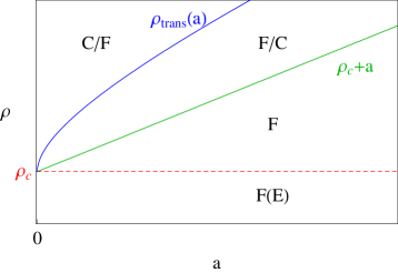
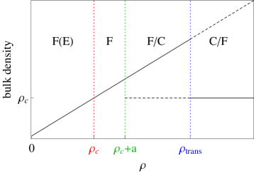
Figure 1: Stationary phase diagram for generic values of $c_{0}>c_{1}$. The four phases $F(E)$ ($\rho\leq\rho_{c}$), $F$ ($\rho_{c}<\rho\leq\rho_{c}+a$), $F/C$ ($\rho_{c}+a<\rho<\rho_{trans}$) and $C/F$ ($\rho\geq\rho_{trans}$) are explained in the text.
Left: Phase diagram in terms of $a$ (5) and the particle density $\rho$. Right: Background density as a function of $\rho$ for $a=0.5$. Full lines are stable, broken lines metastable.

For fixed $L$, also $R$ is a fixed parameter and known results on stationary measures for zero-range processes apply (see e.g. [10] and references therein). The stationary weight $w_{R}^{L}({\boldsymbol{\eta}})$ for this process is of product form,

$$w_{R}^{L}({\boldsymbol{\eta}})=\prod_{x\in\Lambda_{L}}w_{R}({\boldsymbol{\eta}}_{x}),$$ (8)

where the single-site marginal is given by

$$w_{R}(k)=\prod_{i=0}^{k}g_{R}^{-1}(i)=\left\{\begin{array}[]{cl}c_{0}^{-k}&,\ k\leq R\\ c_{0}^{-R}c_{1}^{R-k}&,\ k>R\end{array}\right.\ .$$ (11)

Here the empty product (for $k=0$) is understood to be unity.

The results we derive in the following sections are summarized in the stationary phase diagram in Figure 1 in terms of the conserved particle density $\rho$ and the parameter $a$ (5). In the fluid phases $F(E)$, $F$ and $F/C$ the stationary measure concentrates on homogeneous configurations with bulk density $\rho$. In phase $F(E)$ for $\rho\leq\rho_{c}$ the canonical and grand-canonical ensembles are equivalent (see Section 4), and in phase $F/C$ for $\rho_{c}+a<\rho\leq\rho_{trans}$ there exists an additional metastable condensed phase, which has a lifetime exponential in the system size (see Section 5). Typical condensed configurations have a $\rho$-independent homogeneous bulk distribution with density $\rho_{c}<\rho$, where the excess particles condense on a single lattice site. In phase $C/F$, i.e. for $\rho>\rho_{trans}$, the condensed phase becomes stable and the corresponding fluid phase metastable. On top of metastability the order parameters are discontinuous as a function of the density $\rho$, and therefore the condensation transition is discontinuous.

3 Stationary measures

3.1 Grand-canonical measures

Since the state space $X_{L}$ is discrete we will identify measures $\mu\big{(}\{{\boldsymbol{\eta}}\}\big{)}$ with their mass functions $\mu({\boldsymbol{\eta}})$ in the following to simplify notation. For each $R$ and $L$ there exists a family of stationary product measures $\nu_{\phi,R}^{L}$ with single site marginal

$$\nu^{1}_{\phi,R}(k)=\frac{1}{z_{R}(\phi)}\,w_{R}(k)\,\phi^{k}\ .$$ (12)

The marginal is well defined for fugacities $\phi\in[0,c_{1})$, since the tail behaviour of the stationary weight (11) is $w_{R}(k)\sim c_{1}^{-k}$ for all fixed $R$. The single site normalization is given by the partition function

$$z_{R}(\phi)=\sum_{k=0}^{\infty}w_{R}(k)\,\phi^{k}=\frac{c_{0}}{c_{0}-\phi}\bigg{(}1+\Big{(}\frac{\phi}{c_{0}}\Big{)}^{R+1}\frac{c_{0}-c_{1}}{c_{1}-\phi}\bigg{)}$$ (13)

and the expected particle density under the measure $\nu_{\phi,R}^{L}$ is given by

$$\rho_{R}(\phi) = \big{\langle}\eta_{x}\big{\rangle}_{\nu_{\phi,R}^{1}}=\phi\,\partial_{\phi}\big{(}\log z_{R}(\phi)\big{)}=$$ (14)

$$= \frac{\phi}{c_{0}-\phi}+\Big{(}\frac{\phi}{c_{0}}\Big{)}^{R+1}\frac{R+1+\phi/(c_{1}-\phi)}{\frac{c_{1}-\phi}{c_{0}-c_{1}}+(\phi/c_{0})^{R+1}}\ .$$

Note that $\rho_{R}(\phi)$ is strictly increasing in $\phi$ and that for every fixed $R$, $\rho_{R}(\phi)\to\infty$ as $\phi\to c_{1}$. So for all densities $\rho\geq 0$ there exists $\phi_{R}(\rho)$ such that the measure $\nu_{\phi_{R}(\rho),R}^{L}$ has density $\rho$, i.e. product measures exist for all densities. But the single site marginals of these measures still depend on $R$ and therefore on the system size $L$. Since $R\to\infty$ as $L\to\infty$, the marginal (12) converges pointwise to a simple geometric distribution, i.e. for each $k\in{\mathbb{N}}$,

$$\nu^{1}_{\phi,R}(k)\to\nu^{1}_{\phi,\infty}(k)=\frac{1}{z_{\infty}(\phi)}(\phi/c_{0})^{k}\quad\mbox{with}\quad z_{\infty}(\phi)=\frac{c_{0}}{c_{0}-\phi}\ .$$ (15)

This convergence holds for each fixed $\phi<c_{1}$, but it is not uniform in $\phi$. The limiting product measure $\nu_{\phi,\infty}$ is defined for all $\phi<c_{0}$. We denote the particle density with respect to this measure by

$$\rho_{\infty}(\phi):=\big{\langle}\eta_{x}\big{\rangle}_{\nu_{\phi,\infty}^{1}}=\phi\,\partial_{\phi}\big{(}\log z_{\infty}(\phi)\big{)}=\frac{\phi}{c_{0}-\phi}\ ,$$ (16)

and its inverse is given by

$$\phi_{\infty}(\rho)=c_{0}\,\frac{\rho}{1+\rho}\ .$$ (17)

Since convergence (15) only holds for $\phi<c_{1}$ we define the critical density

$$\rho_{c}:=\rho_{\infty}(c_{1})=\frac{c_{1}}{c_{0}-c_{1}}<\infty\ .$$ (18)

Note that with this definition $\phi_{\infty}(\rho_{c})=c_{1}$. In the following we summarize some straightforward consequences of these definitions.

Proposition 1

For all $\phi<c_{1}$, $\nu^{L}_{\phi,R}\to\nu_{\phi,\infty}$ weakly or, equivalently,

$$\langle f\rangle_{\nu^{L}_{\phi,R}}\to\langle f\rangle_{\nu_{\phi,\infty}}\quad\mbox{as }L\to\infty\mbox{ for all }f\in C_{0,b}(X)\ ,$$ (19)

and $\rho_{R}(\phi)\to\rho_{\infty}(\phi)$. For all $\rho\geq 0$ we have

$$\phi_{R}(\rho)\to\left\{\begin{array}[]{cl}\phi_{\infty}(\rho)&,\ \rho{<}\rho_{c}\\ c_{1}&,\ \rho{\geq}\rho_{c}\end{array}\right.\quad\mbox{and}\quad\nu_{\phi_{R}(\rho),R}^{L}\to\left\{\begin{array}[]{cl}\nu_{\phi_{\infty}(\rho),\infty}&,\ \rho{<}\rho_{c}\\ \nu_{c_{1},\infty}&,\ \rho{\geq}\rho_{c}\end{array}\right.\ ,$$ (24)

where $\phi_{R}$ is the inverse of (14) and the second convergence holds in the weak sense as in (19).

Proof. (15) implies pointwise convergence of arbitrary $n$-point marginals $\nu_{\phi,R}^{n}$ and in general this is equivalent to convergence of expected values of cylinder test functions, as long as they are bounded. This does not directly imply convergence of the unbounded test function $\eta_{x}$ which yields the density, but $\rho_{R}(\phi)\to\rho_{\infty}(\phi)$ follows by direct computation from (14).
Since $\rho_{R}(\phi)$ and its inverse are continuous for $\phi<c_{1}$ or equivalently $\rho<\rho_{c}$, we have $\phi_{R}(\rho)\to\phi_{\infty}(\rho)$. Since $\phi_{\infty}(\rho)<c_{1}$ and $z_{\infty}$ is a continuous function, inserting $\phi_{R}(\rho)$ in (13) yields as $L\to\infty$

$$z_{R}\big{(}\phi_{R}(\rho)\big{)}=z_{\infty}\big{(}\phi_{R}(\rho)\big{)}\bigg{(}1{+}\Big{(}\frac{\phi_{R}(\rho)}{c_{0}}\Big{)}^{R+1}\frac{c_{0}-c_{1}}{c_{1}{-}\phi_{R}(\rho)}\bigg{)}\to z_{\infty}\big{(}\phi_{\infty}(\rho)\big{)}\,.$$ (25)

Therefore, we have pointwise convergence of the marginals as in (15) and $\nu_{\phi_{R}(\rho),R}^{L}\to\nu_{\phi_{\infty}(\rho),\infty}$ weakly for $\rho<\rho_{c}$ analogous to above. For $\rho>\rho_{c}$ to leading order

$$\phi_{R}(\rho)\simeq c_{1}-\Big{(}\frac{c_{1}}{c_{0}}\Big{)}^{R/2}\frac{c_{1}}{\sqrt{z_{\infty}(c_{1})(\rho-\rho_{c})}}\to c_{1}\quad\mbox{as }L\to\infty\ .$$ (26)

For $\rho=\rho_{c}$ the correction has a different power $\big{(}\frac{c_{1}}{c_{0}}\big{)}^{R/4}$ which leads to the same behaviour as for $\rho>\rho_{c}$. Inserting in (13) this yields analogous to (25)

$$z_{R}\big{(}\phi_{R}(\rho)\big{)}=z_{\infty}\big{(}\phi_{R}(\rho)\big{)}\bigg{(}1+\Big{(}\frac{c_{1}}{c_{0}}\Big{)}^{R/2}\sqrt{\frac{\rho-\rho_{c}}{z_{\infty}(c_{1})}}\bigg{)}\to z_{\infty}(c_{1})\quad\mbox{as }L\to\infty$$ (27)

so that $\nu^{L}_{\phi_{R}(\rho),R}\to\nu_{c_{1},\infty}$ weakly. $\Box$

Note that by Proposition 1 the density does not converge if $\rho>\rho_{c}$ since

$$\rho_{R}\big{(}\phi_{R}(\rho)\big{)}=\rho\not\to\rho_{c}=\rho_{\infty}(c_{1})\ ,$$ (28)

and the variance of $\eta_{x}$ even diverges as

$$Var(\eta_{x})=\phi\,\partial_{\phi}\rho_{R}(\phi)\big{|}_{\phi=\phi_{R}(\rho)}\simeq 2c_{1}\Big{(}\frac{c_{0}}{c_{1}}\Big{)}^{R/2-1}$$ (29)

Therefore there is no standard law of large numbers for the measures $\nu^{L}_{\phi_{R}(\rho),R}$ when $\rho>\rho_{c}$. In particular one can show the following.

Proposition 2

For each $L$ let $\eta_{1}^{L},\ldots,\eta_{L}^{L}$ be iid random variables with distribution $\nu^{1}_{\phi_{R}(\rho),R}$ and assume that $R\gg\log L$. Then

$$\frac{1}{L}\sum_{x\in\Lambda_{L}}\eta_{x}^{L}\to\left\{\begin{array}[]{cl}\rho&,\ \rho<\rho_{c}\\ \rho_{c}&,\ \rho\geq\rho_{c}\end{array}\right.\quad\mbox{almost surely}\ .$$ (32)

Proof. see appendix

Note that for $\rho>\rho_{c}$ (28) holds due to very large values $\eta_{x}\sim\big{(}\frac{c_{0}}{c_{1}}\big{)}^{R/2}$ having very small probabilities $\big{(}\frac{c_{1}}{c_{0}}\big{)}^{R/2}$, which also leads to divergence of the variance (29). In turn, the small probabilities lead to almost sure convergence of the sample mean to $\rho_{c}<\rho$, which is a non-standard strong law of large numbers. The breakdown of the standard strong law coincides with the region of nonequivalence of ensembles, as has been observed also in the context of spin systems [8, 31].

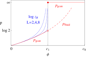
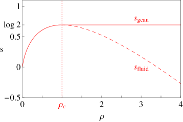
Figure 2: Properties of fluid and grand-canonical measures for $c_{0}=2$, $c_{1}=1$ as given in (33) to (40). Left: Pressure $p_{gcan}$ (full red line), $p_{fluid}$ (broken red line) and $\log z_{R}$ for $L=2,4,8$ (dashed blue lines), demonstrating the fast convergence to $p_{gcan}$. Right: Entropy densities $s_{gcan}$ (full red line) and $s_{fluid}$ (broken red line).

As noted before, the limiting product measures $\nu_{\phi,\infty}$ (15) exist for all $\phi<c_{0}$ and for reasons explained below, we call the family of measures $\big{\{}\nu_{\phi_{\infty}(\rho),\infty}\,:\,\rho\geq 0\big{\}}$ the fluid phase. The pressure of the fluid phase is given by

$$p_{fluid}(\phi):=\lim_{L\to\infty}\frac{1}{L}\log z_{\infty}^{L}(\phi)=\log z_{\infty}(\phi)=\log\frac{c_{0}}{c_{0}-\phi}$$ (33)

and we define the entropy density by the negative Legendre transform

$$s_{fluid}(\rho) := -\sup_{\phi\geq 0}\big{(}\rho\,\log\phi-p_{fluid}(\phi)\big{)}=p\big{(}\phi_{\infty}(\rho)\big{)}-\rho\log\phi_{\infty}(\rho)=$$ (34)

$$= (1+\rho)\log(1+\rho)-\rho(\log c_{0}+\log\rho)\ ,$$

where the supremum is attained for $\phi=\phi_{\infty}(\rho)$ (17). Note that the fluid pressure and entropy density are different from the grand-canonical quantities, because $z_{R}(\phi)=\infty$ for $\phi\geq c_{1}$ (13). This yields

$$p_{gcan}(\phi):=\lim_{L\to\infty}\frac{1}{L}\log z_{R}^{L}(\phi)=\left\{\begin{array}[]{cl}p_{fluid}(\phi)&,\ \phi<c_{1}\\ \infty&,\ \phi\geq c_{1}\end{array}\right.$$ (37)

and the negative Legendre transform of the pressure is given by

$$s_{gcan}(\rho)=\left\{\begin{array}[]{cl}s_{fluid}(\rho)&,\ \rho\leq\rho_{c}\\ s_{fluid}(\rho_{c})-(\rho-\rho_{c})\log c_{1}&,\ \rho>\rho_{c}\end{array}\right.\ .$$ (40)

Note that the Legendre transform of the pressure is usually called the free energy density. In thermodynamics, the free energy $F$ is related to the entropy $S$ via $F=U-TS$, where $U$ is the internal energy and $T$ the temperature. Since there is no energy and temperature in our case, we define the entropy density as the negative free energy density. The functions (33) to (40) are illustrated in Figure 2. In analogy to previous results [17, 16] we expect a condensation transition for $\rho>\rho_{c}$. But the non-standard behaviour of the grand-canonical measures, in particular the lack of a law of large numbers (32), will lead to a richer behaviour than in previous studies, which can be fully understood only in the context of the equivalence of ensembles. In particular, the grand-canonical approach alone does not provide a complete picture of the phase transition.

3.2 Canonical measures

The canonical measures are given by

$$\pi_{L,N}:=\nu_{\phi,R}^{L}(\,.\,|\,\Sigma_{L}=N)\quad\mbox{where}\quad\Sigma_{L}({\boldsymbol{\eta}}):=\sum_{x\in\Lambda_{L}}\eta_{x}\ ,$$ (41)

i.e. they are given by a grand-canonical measure conditioned on a fixed number $N$ of particles. Their mass functions are independent of $\phi$ and given in terms of the stationary weights (8) by

$$\pi_{L,N}({\boldsymbol{\eta}})=\frac{1}{Z_{L,N}}\,w_{R}^{L}({\boldsymbol{\eta}})\,\delta(\Sigma_{L}({\boldsymbol{\eta}}),N)\ ,$$ (42)

concentrating on configurations

$$X_{L,N}=\big{\{}{\boldsymbol{\eta}}\in X_{L}\,\big{|}\,\Sigma_{L}({\boldsymbol{\eta}})=N\big{\}}\ .$$ (43)

The partition function is now given by the finite sum

$$Z_{L,N}=w_{R}^{L}(X_{L,N})=\sum_{{\boldsymbol{\eta}}\in X_{L,N}}w_{R}^{L}({\boldsymbol{\eta}})\ .$$ (44)

In the following we analyze the limiting behaviour of this quantity. In the discussion configurations with many particles on a small number of sites turn out to play an important role. Therefore we define the disjoint sets of configurations

$$X_{L,N}^{m}=\big{\{}{\boldsymbol{\eta}}\in X_{L,N}\,\big{|}\,\eta_{x}>R\mbox{ for exactly }m\mbox{ sites }x\in\Lambda_{L}\big{\}}\$$ (45)

with more than $R$ particles on exactly $m$ sites.

Theorem 1

Suppose $R\gg\log L$, i.e. $\frac{\log L}{R}\to 0$ as $L\to\infty$. Then the limit

$$s_{can}(\rho):=\lim_{L\to\infty}\frac{1}{L}\log Z_{L,N}\ ,\quad\mbox{where }N/L\to\rho\ ,$$ (46)

exists and is called the canonical entropy density. It is given by

$$s_{can}(\rho)=\left\{\begin{array}[]{cl}s_{fluid}(\rho)&,\ \rho\leq\rho_{trans}\\ s_{fluid}(\rho_{c})+s_{cond}(\rho,\rho_{c})&,\ \rho>\rho_{trans}\end{array}\right.\ ,$$ (49)

where

$$s_{cond}(\rho,\rho_{c})=\lim_{L\to\infty}\frac{1}{L}\log w_{R}\big{(}(\rho-\rho_{c})L\big{)}\ .$$ (50)

The transition density $\rho_{trans}(a)$ is given by the unique solution of

$$a=\Big{(}s_{fluid}(\rho_{c})-(\rho-\rho_{c})\log c_{1}-s_{fluid}(\rho)\Big{)}\Big{/}\log\frac{c_{0}}{c_{1}}\ ,$$ (51)

where $\rho_{trans}(a)\geq\rho_{c}+a$ with equality if and only if $a=0$.

Note that with (50) and (11) the contribution of the condensate to the canonical entropy is given by

$$s_{cond}(\rho,\rho_{c})=-(\rho-\rho_{c})\log c_{1}-a\log\frac{c_{0}}{c_{1}}\ .$$ (52)

As a special case, taking $a=0$ we have $\rho_{trans}=\rho_{c}$ as the unique solution of (51), and comparing (49) with (40) yields

$$s_{can}(\rho)=s_{gcan}(\rho)\quad\mbox{for all }\rho\geq 0\ .$$ (53)

On the other hand, both entropies are different whenever $a>0$.

Proof of Theorem 1. Using (45) we decompose the state space $X_{L,N}=\bigcup_{m=0}^{M}X_{L,N}^{m}$. The maximal number $M$ of sites containing more than $R$ particles is certainly bounded by $M=:\lceil N/R\rceil$. Notice that $M\to\rho/a\in(0,\infty]$ as $L\to\infty$, and in particular $M/L\to 0$. We can estimate the number of “uncondensed” configurations where no site has more than $R$ particles by the following Lemma, which is proved in the appendix.

Lemma 1

For all $L,N\geq 1$ and $M$ as above we have

$$\frac{|X_{L,N}|}{1+{L+M\choose M}\big{/}(L-M)^{R}}\leq|X_{L,N}^{0}|\leq|X_{L,N}|\ .$$ (54)

This includes for all $\rho\geq 0$ and $N/L\to\rho$

$$\lim_{L\to\infty}\frac{1}{L}\log|X_{L,N}^{0}|=\lim_{L\to\infty}\frac{1}{L}\log|X_{L,N}|=\chi(\rho)\ ,$$ (55)

where $\chi(\rho):=(1+\rho)\log(1+\rho)-\rho\log\rho$.
Furthermore, if $R\gg\sqrt{L}$, then $\lim\limits_{L\to\infty}|X_{L,N}^{0}|/|X_{L,N}|=1$ for all $\rho\geq 0$.

Now we split the partition function accordingly

$$Z_{L,N}=\sum_{m=0}^{M}Z_{L,N}^{m}\ ,\quad\mbox{where}\quad Z_{L,N}^{m}=w_{R}^{L}(X_{L,N}^{m})\ .$$ (56)

For the term $m=0$ we get with Lemma 1

$$\frac{1}{L}\log Z_{L,N}^{0}=\frac{1}{L}\log\big{(}c_{0}^{-N}|X_{L,N}^{0}|\big{)}\to\chi(\rho)-\rho\log c_{0}=s_{fluid}(\rho)\ .$$ (57)

The contributions of the other terms are given by

$$Z_{L,N}^{m}{=}{L\choose m}c_{0}^{-mR}\!\!\!\sum_{k=m(R+1)}^{N}\!\!\!c_{0}^{-(N-k)}\,c_{1}^{-(k-mR)}\,\big{|}X_{L-m,N-k}^{0}\big{|}{k{-}mR{-}1\choose m{-}1}.$$ (58)

Here we have chosen $m$ sites on which we distribute $k$ particles such that each site contains at least $R+1$ particles, giving rise to the first and last combinatorial factor. The $N-k$ remaining particles are distributed on $L-m$ sites such that none contains more than $R$ particles. The sum can be approximated by an integral and evaluated by the saddle point method. The saddle point equation reads

$$\log\frac{c_{0}}{c_{1}}-\frac{L}{L-m}\ \chi^{\prime}\Big{(}\frac{N-k}{L-m}\Big{)}+\log\frac{k-mR-1}{k-m(R+1)}=0\ .$$ (59)

This has a solution if and only if

$$N-(L-m)\rho_{c}\geq m(R+1)\quad\mbox{or, equivalently}\quad\rho\geq\rho_{c}+m\,a\ .$$ (60)

In this case, to leading order the solution to (59) is given by

$$k\simeq N-(L-m)\rho_{c}$$ (61)

where we have used that $m/L\to 0$ for all $m\leq M$. On the other hand, for $\rho<\rho_{c}+m\,a$ the sum in (58) is maximized for the boundary value $k=m(R+1)$. We get in leading exponential order

$$Z_{L,N}^{m}\simeq\left\{\begin{array}[]{cl}0&,\ \rho\leq m\,a\\ {L\choose m}\big{(}\frac{c_{0}}{c_{1}}\big{)}^{m}c_{0}^{-N}e^{(L-m)\chi(\rho-ma)}&,\ m\,a{<}\rho{<}\rho_{c}{+}m\,a\\ {L\choose m}\big{(}\frac{c_{1}}{c_{0}}\big{)}^{mR+(L-m)\rho_{c}}c_{1}^{-N}e^{(L-m)\chi(\rho_{c})}&,\ \rho\geq\rho_{c}+m\,a\end{array}\right.\ .$$ (65)

For $\rho>\rho_{c}+a$ we get a rough estimate by adding both cases,

$$\sum_{m=2}^{M}Z_{L,N}^{m}\leq Z_{L,N}^{1}{L\choose M}\bigg{(}\frac{M}{L}\Big{(}\frac{c_{1}}{c_{0}}\Big{)}^{N-M-R-(L-1)\rho_{c}}{+}\Big{(}\frac{c_{1}}{c_{0}}\Big{)}^{R}CL^{M-2}\bigg{)}\,,$$ (66)

where $C=\exp\Big{(}(c_{0}/c_{1})^{\rho_{c}}e^{-\chi(\rho_{c})}\Big{)}$. Now, to leading order

$$\frac{1}{L}\log\Bigg{(}{L\choose M}\Big{(}\frac{c_{1}}{c_{0}}\Big{)}^{R}C\,L^{M-2}\Bigg{)}\simeq-\frac{M}{L}\Big{(}1+\log\frac{M}{L}+\frac{M}{L}\Big{)}-\frac{\log L}{L}$$ (67)

$$\quad-\frac{R}{L}\log\frac{c_{0}}{c_{1}}+\frac{M}{L}\log L\ \to\ -a\log\frac{c_{0}}{c_{1}}\leq 0\quad\mbox{as }L\to\infty\ ,$$

since $M/L\to 0$, $R/L\to a\geq 0$. This holds only if $M\ll L/\log L$ or, equivalently, $R\gg\log L$. Since $\rho>\rho_{c}+a$ the first summand on the right-hand side of (66) vanishes with an analogous argument. Therefore

$$\frac{1}{L}\log\bigg{(}1+\sum_{m=2}^{M}Z_{L,N}^{m}\Big{/}Z_{L,N}^{1}\bigg{)}\to 0\ ,$$ (68)

and the only exponential contribution to (66) is given by $Z_{L,N}^{1}$. Thus we have, using (65),

$$\lim_{L\to\infty}\frac{1}{L}\log\sum_{m=1}^{M}Z_{L,N}^{m}=\lim_{L\to\infty}\frac{1}{L}\log Z_{L,N}^{1}=$$ (69)

$$\quad=\lim_{L\to\infty}\frac{1}{L}\log\bigg{(}L\Big{(}\frac{c_{1}}{c_{0}}\Big{)}^{R+(L-1)\rho_{c}}c_{1}^{-N}\big{|}X^{0}_{L-1,(L-1)\rho_{c}}\big{|}\bigg{)}=$$

$$\quad=(a+\rho_{c})\log\frac{c_{1}}{c_{0}}-\rho\log c_{1}+\chi(\rho_{c})=s_{fluid}(\rho_{c})+s_{cond}(\rho,\rho_{c})\ .$$

This is a linear function in $\rho$ with the same slope $-\log c_{1}$ as $s_{gcan}(\rho)$ (40). Note that for $\rho\to\infty$ the first term (57) behaves as

$$s_{fluid}(\rho)\simeq-\rho\log c_{0}+\log(1+\rho)+1\ .$$ (70)

Therefore, whereas for small $\rho$ (57) dominates the partition function, (69) dominates for large $\rho$, since it has larger asymptotic slope $-\log c_{1}>-\log c_{0}$. The transition density $\rho_{trans}$ as a function of $a$ is found by equating both contributions which leads directly to (51). Differentiating the right-hand side of this equation yields

$$a^{\prime}(\rho)=1-\log\frac{1+\rho}{\rho}\Big{/}\log\frac{c_{0}}{c_{1}}\ .$$ (71)

Thus $a^{\prime}(\rho_{c})=0$ and $a^{\prime}(\rho)\in(0,1)$ for all $\rho>\rho_{c}$. Since also $a(\rho_{c})=0$, (51) has a unique solution $\rho_{trans}(a)\geq\rho_{c}$ for all $a\geq 0$. Further we have

$$\rho^{\prime}_{trans}(a)=\frac{1}{a^{\prime}(\rho_{trans}(a))}>1\quad\mbox{for all}\quad\rho\geq\rho_{c}\ ,$$ (72)

and thus $\rho_{trans}(a)\geq\rho_{c}+a$ with equality if and only if $a=0$. $\Box$

Now, if $a>0$ then $M$ as defined after (45) is bounded and converges to $\rho/a$, and thus (66) implies that

$$\sum_{m=2}^{M}Z_{L,N}^{m}\Big{/}Z_{L,N}^{1}\to 0\quad\mbox{as}\quad L\to\infty\ .$$ (73)

This is significantly stronger than (67) and it is easy to see that it still holds for $a=0$, as long as $R\gg\sqrt{L\log L}$. Thus for $L\to\infty$ the canonical measure concentrates on certain parts of the state space, and from the proof of Theorem 1 (66) the rate of convergence is faster than polynomial in $L$. Therefore we can immediately deduce the following.

Corollary 1

For $R\gg\sqrt{L\log L}$ we have

$$\rho<\rho_{trans}\quad \Rightarrow \quad\pi_{L,N}\big{(}X_{L,N}^{0}\big{)}\to 1\ ,\quad L^{n}\pi_{L,N}\big{(}X_{L,N}\setminus X_{L,N}^{0}\big{)}\to 0\ ,$$

$$\rho>\rho_{trans}\quad \Rightarrow \quad\pi_{L,N}\big{(}X_{L,N}^{1}\big{)}\to 1\ ,\quad L^{n}\pi_{L,N}\big{(}X_{L,N}\setminus X_{L,N}^{1}\big{)}\to 0\ ,$$ (74)

for all $n\in{\mathbb{N}}$ as $L\to\infty$ and $N/L\to\rho$.

This implies in analogy to (49), that for $\rho>\rho_{trans}$ a typical configuration consists of a homogeneous background with density $\rho_{c}$ and the $(\rho-\rho_{c})L$ excess particles concentrate in a single lattice site. We expect this kind of behaviour actually already for $R\gg\log L$, since $w_{R}$ has an exponential tail and maximal fluctuations under $w_{R}^{L}$ in the occupation number are of order $\log L$. Our estimates are not strong enough to deduce this, but we are primarily interested in $a>0$, which is covered by the above result. The same is true for the last statement of Lemma 1.
For $\rho=\rho_{trans}$ the contributions of condensed and fluid configurations to the canonical entropy are equal (49). This is true on the exponential scale and to deduce the behaviour on the transition line we need a finer estimate, given in the following Theorem.

Theorem 2

For $N/L\to\rho_{trans}$ and $a>0$ we have

$$w_{R}^{L}(X_{L,N}^{1})/w_{R}^{L}(X_{L,N}^{0})=O(L^{3/2})\to\infty\quad\mbox{as }L\to\infty\ ,$$ (75)

which implies $\pi_{L,N}(X_{L,N}^{1})\to 1$.

So in case of a discontinuous transition (i.e. $a>0$) the transition line belongs to the condensed phase $C/F$. For $a=0$ the transition is continuous and therefore $\rho=\rho_{c}$ belongs to the fluid phase $F(E)$.

Proof. According to (58) in the proof of Theorem 1,

$$w_{R}^{L}(X_{L,N}^{1}) = L\,c_{0}^{-R}\sum_{k=R+1}^{N}c_{0}^{-(N-k)}\,c_{1}^{-(k-R)}\,\big{|}X_{L-1,N-k}^{0}\big{|}=$$ (76)

$$= L\Big{(}\frac{c_{1}}{c_{0}}\Big{)}^{R+\rho_{c}(L-1)}c_{1}^{-N}\big{|}X_{L-1,\rho_{c}(L-1)}^{0}\big{|}\,\big{(}1+o(1)\big{)}$$

$$\int_{R+1}^{N}\exp\bigg{(}\frac{1}{2}\,\chi^{\prime\prime}(\rho_{c})\frac{L}{(L-1)^{2}}(k-\bar{k})^{2}\bigg{)}dk$$

where $\bar{k}=N-(L-1)\rho_{c}+o(L)$ is the solution to the saddle point equation (59). In addition to the proof of Theorem 1 we consider the next order of the expansion to get the correct asymptotic behaviour. Since with Lemma 1, $\chi^{\prime\prime}(\rho)=-\frac{1}{\rho(1+\rho)}<0$ for all $\rho>0$ and $\bar{k}\in(R+1,N)$, the asymptotic behaviour of the Gaussian integral with variance $\sigma^{2}=-L/\chi^{\prime\prime}(\rho_{c})(1+o(1))$ is given by its normalization and we get

$$w_{R}^{L}(X_{L,N}^{1})=$$ (77)

$$=L^{3/2}\Big{(}\frac{c_{1}}{c_{0}}\Big{)}^{R+\rho_{c}(L-1)}c_{1}^{-N}\big{|}X_{L-1,\rho_{c}(L-1)}^{0}\big{|}\,\sqrt{2\pi\rho_{c}(1+\rho_{c})}\big{(}1+o(1)\big{)}\ .$$

With $C=\sqrt{2\pi\rho_{c}(1+\rho_{c})}$ this leads to

$$\frac{w_{R}^{L}(X_{L,N}^{1})}{w_{R}^{L}(X_{L,N}^{0})} = CL^{3/2}\frac{\big{(}\frac{c_{1}}{c_{0}}\big{)}^{R+\rho_{c}L}c_{1}^{-N}\big{|}X_{L-1,\rho_{c}(L-1)}^{0}\big{|}}{c_{0}^{-N}\big{|}X_{L,N}^{0}\big{|}}\big{(}1+o(1)\big{)}=$$ (78)

$$= CL^{3/2}\frac{\big{(}\frac{c_{1}}{c_{0}}\big{)}^{R+\rho_{c}L}c_{1}^{-N}{(L-1)(1+\rho_{c})-1\choose L-2}}{c_{0}^{-N}{L+N-1\choose L-1}}\big{(}1+o(1)\big{)}\ ,$$

where we have used the third statement of Lemma 1 that holds for $a>0$. We use Stirling’s formula for the binomial coefficients and note that due to Theorem 1 the exponential terms in the ratio vanish, which leaves us with

$$\frac{w_{R}^{L}(X_{L,N}^{1})}{w_{R}^{L}(X_{L,N}^{0})}=CL^{3/2}\big{(}1+o(1)\big{)}\to\infty\quad\mbox{as }L\to\infty,N/L\to\rho_{trans}\ .$$ (79)

Together with Theorem 1 this implies that

$$w_{R}^{L}(X_{L,N}\setminus X_{L,N}^{1})\to 0\quad\mbox{as }L\to\infty,N/L\to\rho_{trans}\ ,$$ (80)

which implies the last statement of the Theorem. $\Box$

4 Equivalence of ensembles

4.1 Specific relative entropy

	canonical entropy	grand-canonical entropy
phase	$s_{can}(\rho)$	$s_{gcan}(\rho)$
F(E)	$s_{fluid}(\rho)$	$s_{fluid}(\rho)$
F, F/C	$s_{fluid}(\rho)$
C/F	$s_{fluid}(\rho_{c}){-}(\rho{-}\rho_{c})\log c_{1}{-}a\log\frac{c_{0}}{c_{1}}$	$s_{fluid}(\rho_{c}){-}(\rho{-}\rho_{c})\log c_{1}$

Table 1: Summary of the results of Section 3: Comparison between canonical and grand-canonical entropy density. Equivalence of ensembles holds only in phase $F(E)$.

In Table 1 we summarize the results of the previous section in connection with the phase diagram shown in Figure 1. In particular, for $a=0$ the phases $F$ and $F/C$ are empty since $\rho_{c}=\rho_{trans}$, and we have $s_{can}(\rho)=s_{gcan}(\rho)$ for all $\rho\geq 0$ as noted already in (53). This implies that the canonical entropy density is concave and the condensation transition is continuous. On the other hand, for $a>0$ we have equivalence of ensembles only in phase $F(E)$, the canonical entropy density is non-concave, and the transition is discontinuous. These results concern equivalence of ensembles in terms of convergence of entropies of the canonical and the grand-canonical measure. In Figure 3 they are illustrated by numerical calculations of the canonical entropy density using the recursion relation

$$Z_{L,N}=\sum_{k=0}^{N}w_{R}(k)Z_{L-1,N-k}\ .$$ (81)

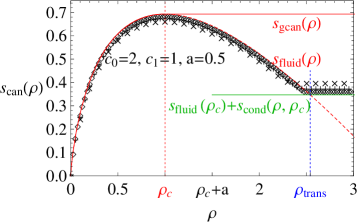
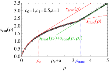
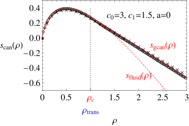
Figure 3: Canonical entropy density $s_{can}(\rho)$ for various values of $c_{0}$, $c_{1}$ and $a$. Data points are calculated numerically according to (81) with $L=100\ (\times)$, $200\ (+)$, $400\ (\Diamond)$, and show good agreement with the theoretical predictions for the thermodynamic limit (see Table 1).

As can be seen, the grand-canonical entropy density is equal to the concave hull of $s_{can}(\rho)$ which itself is not concave for $a>0$. The canonical entropy density further coincides with the one of the fluid phase, up to the point when it becomes metastable and the condensed phase becomes stable. This point has been derived exactly by studying the dominating terms in the canonical partition function.

We can make a connection to other formulations of the equivalence of ensembles, using the specific relative entropy

$$h(\pi_{L,N},\nu_{\phi,R}^{L}):=\frac{1}{L}\,H(\pi_{L,N},\nu_{\phi,R}^{L})=\frac{1}{L}\,\Big{\langle}\log\frac{\pi_{L,N}({\boldsymbol{\eta}})}{\nu_{\phi,R}^{L}({\boldsymbol{\eta}})}\Big{\rangle}_{\pi_{L,N}}\ .$$ (82)

With the identity $\pi_{L,N}^{L}=\nu_{\phi,R}^{L}(\,.\,|\,\Sigma_{L}=N)$, this can be expressed in two useful forms,

$$h(\pi_{L,N},\nu_{\phi,R}^{L}) = -\frac{1}{L}\log\nu_{\phi,R}^{L}\big{(}\Sigma_{L}=N\big{)}=$$ (83)

$$= \log z_{R}(\phi)-\frac{N}{L}\,\log\phi-\frac{1}{L}\,\log Z_{L,N}\ .$$

The derivation of these expressions is straightforward, see e.g. [17]. The following is a direct consequence of our results on the canonical measure in Theorem 1.

Corollary 2

Choosing $\phi=\phi_{R}(\rho)$ according to (24) we get for all $\rho\geq 0$

$$h(\pi_{L,N},\nu_{\phi_{R}(\rho),R}^{L})\to s_{gcan}(\rho)-s_{can}(\rho)\ .$$ (84)

Proof. We use the second expression in (83) for the specific relative entropy. Choosing $\phi=\phi_{R}(\rho)$, the first two terms converge

$$\log z_{R}(\phi_{R}(\rho))-\log\phi_{R}(\rho)\,\frac{N}{L}\to s_{gcan}(\rho)$$ (85)

to the grand-canonical entropy density (40), since with Proposition 1, analogous to (25) and (27)

$$z_{R}\big{(}\phi_{R}(\rho)\big{)}\to\left\{\begin{array}[]{cl}z_{\infty}\big{(}\phi_{\infty}(\rho)\big{)}&,\mbox{ for }\rho<\rho_{c}\\ z_{\infty}(c_{1})&,\mbox{ for }\rho\geq\rho_{c}\end{array}\right.\ .$$ (88)

Convergence of the third term in (83) has been shown in Theorem 1, which finishes the proof. $\Box$

We can read from Table 1 that

$$s_{gcan}(\rho){-}s_{can}(\rho)=\left\{\begin{array}[]{cl}0&,\,\rho\leq\rho_{c}\\ \!\!\ s_{fluid}(\rho_{c}){-}s_{fluid}(\rho){-}(\rho{-}\rho_{c})\log c_{1}&,\,\rho_{c}{<}\rho{<}\rho_{trans}\\ a\log(c_{0}/c_{1})&,\,\rho\geq\rho_{trans}\end{array}\right..$$ (92)

In particular, for $a=0$ we have $\rho_{c}=\rho_{trans}$ and

$$h(\pi_{L,N},\nu_{\phi_{R}(\rho),R}^{L})\to 0\quad\mbox{for all }\rho\geq 0\ ,$$ (93)

whereas for $a>0$ this holds only for $\rho\leq\rho_{c}$. By a standard result [6], convergence in specific relative entropy implies weak convergence, i.e. convergence of expectations of bounded cylinder test functions $f\in C_{0,b}(X)$,

$$\Big{|}\langle f\rangle_{\pi_{L,N}}-\langle f\rangle_{\nu_{\phi_{R}(\rho),R}^{L}}\Big{|}\to 0\quad\mbox{as }L\to\infty\ ,N/L\to\rho\ .$$ (94)

This is another formulation of the equivalence of ensembles.

Furthermore, we can compare the canonical measures with the expected fluid measures for the background.

Theorem 3

Let $a>0$. Choosing $\phi=\phi_{\infty}(\rho)$ according to (17) we get

$$h(\pi_{L,N},\nu_{\phi_{\infty}(\rho),\infty}^{L})\to s_{fluid}(\rho)-s_{can}(\rho)=0\quad\mbox{for }0\leq\rho<\rho_{trans}\ ,$$ (95)

whereas for $\phi=c_{1}$

$$h(\pi_{L,N},\nu_{c_{1},\infty}^{L})\to(\rho-\rho_{c})\log\frac{c_{0}}{c_{1}}>0\quad\mbox{for }\rho\geq\rho_{trans}\ .$$ (96)

Now let $a=0$ and $R\gg\sqrt{L\log L}$. We have $\rho_{trans}=\rho_{c}$ and (95) holds for $0\leq\rho\leq\rho_{c}$, (96) for $\rho>\rho_{c}$.

Proof. According to the definition (82) we have

$$h(\pi_{L,N},\nu_{\phi_{\infty}(\rho),\infty}^{L})=\frac{1}{L}\sum_{{\boldsymbol{\eta}}\in X_{L,N}}\pi_{L,N}({\boldsymbol{\eta}})\log\frac{\pi_{L,N}({\boldsymbol{\eta}})}{\nu_{\phi_{\infty}(\rho),\infty}^{L}({\boldsymbol{\eta}})}=p_{fluid}\big{(}\phi_{\infty}(\rho)\big{)}$$ (97)

$$\quad-\frac{N}{L}\,\log\frac{\phi_{\infty}(\rho)}{c_{0}}-\frac{1}{L}\,\log Z_{L,N}+\frac{1}{L}\sum_{{\boldsymbol{\eta}}\in X_{L,N}}\pi_{L,N}({\boldsymbol{\eta}})\log w_{R}^{L}({\boldsymbol{\eta}})\ ,$$

where we have used the definitions (15) and (42),

$$\nu^{1}_{\phi,\infty}(k)=\frac{1}{z_{\infty}(\phi)}(\phi/c_{0})^{k}\ ,\quad\pi_{L,N}({\boldsymbol{\eta}})=\frac{1}{Z_{L,N}}\,w_{R}^{L}({\boldsymbol{\eta}})\,\delta(\Sigma_{L}({\boldsymbol{\eta}}),N)\ .$$ (98)

Splitting the last term of (97) and using Corollary 1 we see that

$$\frac{1}{L}\sum_{{\boldsymbol{\eta}}\in X^{0}_{L,N}}\!\!\!\pi_{L,N}({\boldsymbol{\eta}})\log c_{0}^{-N}+\frac{1}{L}\!\!\!\sum_{{\boldsymbol{\eta}}\in X_{L,N}\setminus X_{L,N}^{0}}\!\!\!\!\!\!\!\!\!\!\pi_{L,N}({\boldsymbol{\eta}})\log w_{R}^{L}({\boldsymbol{\eta}})\to{-}\rho\log c_{0}\,,$$ (99)

as $L\to\infty$, $N/L\to\rho$, as long as $\rho<\rho_{trans}$. Therefore, with definition (34),

$$h(\pi_{L,N},\nu_{\phi_{\infty}(\rho),\infty}^{L})\to s_{fluid}(\rho)-s_{can}(\rho)=0\quad\mbox{for }\rho<\rho_{trans}\ .$$ (100)

This holds for all $a\geq 0$ as long as $R\gg\sqrt{L\log L}$. For $\rho>\rho_{trans}$ we also use (97) where $\phi_{\infty}(\rho)$ is replaced by $c_{1}$. Again with Corollary 1 the main contribution to the last term comes now from ${\boldsymbol{\eta}}\in X^{1}_{L,N}$. The sum can be computed by the saddle point method analogous to the proof of Theorem 1 and we get

$$\frac{1}{L}\sum_{{\boldsymbol{\eta}}\in X^{1}_{L,N}}\pi_{L,N}({\boldsymbol{\eta}})\log w_{R}^{L}({\boldsymbol{\eta}})\to a\log\frac{c_{1}}{c_{0}}-\rho_{c}\log c_{0}-(\rho-\rho_{c})\log c_{1}\ .$$ (101)

The same also holds for $\rho=\rho_{trans}$, since with Theorem 2 $\pi_{L,N}$ concentrates on $X_{L,N}^{1}$ also in this case. The first terms in (97) are now

$$p_{fluid}\big{(}c_{1}\big{)}-\frac{N}{L}\,\log\frac{c_{1}}{c_{0}}\to s_{fluid}(\rho_{c})+\rho\log c_{0}-(\rho-\rho_{c})\log c_{1}\ ,$$ (102)

and together with the behaviour of $s_{can}$ from Theorem 1 we get for $\rho\geq\rho_{trans}$

$$h(\pi_{L,N},\nu_{c_{1},\infty}^{L})\to(\rho-\rho_{c})\log\frac{c_{0}}{c_{1}}>0\ ,$$ (103)

finishing the proof of Theorem 3. Note that $a=0$ is included as a special case in the above derivation as long as $R\gg\sqrt{L\log L}$. $\Box$

(95) allows us to identify the limit measure and we have

$$\langle f\rangle_{\pi_{L,N}}\to\langle f\rangle_{\nu_{\phi_{\infty}(\rho),\infty}}\quad\mbox{as }L\to\infty\ ,\quad N/L\to\rho\ .$$ (104)

As a direct consequence of the relative entropy inequality ([5], Lemma 3.1), this holds not only for bounded cylinder test functions $f$, but for the larger class with $\langle e^{\epsilon f}\rangle_{\nu_{\phi_{\infty}(\rho),\infty}}<\infty$ for some $\epsilon>0$. Since the fluid measures have finite exponential moments, this includes local occupation numbers $f({\boldsymbol{\eta}})=\eta_{x}$, which are unbounded. This ensures convergence of densities for $\rho<\rho_{trans}$ ($\rho\leq\rho_{c}$ for $a=0$), i.e. in the fluid phases $F(E)$, $F$ and $F/C$.

4.2 The condensed phase

(96) may suggest that the limiting distribution of the background in the condensed phase $C/F$ is more complicated than the expected fluid measure $\nu_{c_{1},\infty}$. Together with Corollary 1 we can show that the non-zero specific relative entropy is only due to the contribution of the single condensate site and indeed the background distribution is as expected. In the following we attach some (arbitrary) ordering to the lattice sites and identify $\Lambda_{L}=\{1,\ldots,L\}$. On $X_{L-1}$ we define the measure $\hat{\pi}_{L,N}$ as a marginal on the first $L-1$ coordinates

$$\hat{\pi}_{L,N}:=\pi_{L,N}(.|L\in\mathrm{argmax})^{1,..,L{-}1}$$ (105)

where $\pi_{L,N}(.|L\in\mathrm{argmax})$ denotes the measure $\pi_{L,N}$ conditioned on the event that $\eta_{L}\geq\eta_{x}$ for all $x=1,\ldots,L-1$. Since $\pi_{L,N}$ is invariant under site permutations, we have

$$\hat{\pi}_{L,N}:=\pi_{L,N}(.|y\in\mathrm{argmax})^{\Lambda_{L}\setminus\{y\}}\quad\mbox{for all }y\in\Lambda_{L}\ .$$ (106)

Note that $\hat{\pi}_{L,N}$ concentrates on a subset of $X_{L-1}$,

$$\hat{X}_{L-1}:=\big{\{}\hat{\boldsymbol{\eta}}\in X_{L-1}\,\big{|}\,\Sigma_{L-1}(\hat{\boldsymbol{\eta}})<N,\,\hat{\eta}_{1},..,\hat{\eta}_{L-1}\leq N-\Sigma_{L-1}(\hat{\boldsymbol{\eta}})\big{\}}\ ,$$ (107)

and in case of condensation it can be interpreted as the distribution of the background.

Theorem 4

For $\rho\geq\rho_{trans}$ we have as $L\to\infty$, $N/L\to\rho$,

$$H(\hat{\pi}_{L,N},\nu_{c_{1},\infty}^{L-1})\to 0\ ,$$ (108)

and thus for bounded cylinder test functions

$$\langle f\rangle_{\pi_{L,N}}\to\langle f\rangle_{\nu_{c_{1},\infty}}\ .$$ (109)

Note that the first statement (108) involves the total rather than the specific relative entropy and is therefore much stronger than Corollary 2 and Theorem 3. This implies convergence in total variation norm [5]. Such a result is not possible below criticality, since the conditioning on the particle number in the canonical measures leads to divergence of the relative entropy. Above criticality, this condition is accounted for purely by the condensate site and does not affect the background, which shows the same fluctuations as i.i.d. random variables. Following recent results in [24], this enables to show that the stationary density profiles converge to a Brownian motion with a jump at the location of the condensate. Below criticality the corresponding expected behaviour would be a Brownian bridge, but there is no proof so far.
The second statement (109) is a direct consequence of the first but not a very strong one, since it would also follow from convergence in specific relative entropy. The site with maximum occupation number will be in the support of the cylinder test function only with probability of order $1/L$. But due to this possibility, the test function has to be bounded, not necessarily by a constant but by a number of order $o(L)$. This excludes $f({\boldsymbol{\eta}})=\eta_{x}$ as expected, since the expected density does not converge for $\rho\geq\rho_{trans}$. Note also that with (96) and (109) this system is an example where weak convergence is strictly weaker than convergence in specific relative entropy.

Proof. (105) and (107) imply that

$$\hat{\pi}_{L,N}(\hat{\boldsymbol{\eta}})=\frac{\pi_{L,N}\big{(}\hat{\boldsymbol{\eta}},N-\Sigma_{L-1}(\hat{\boldsymbol{\eta}})\big{)}}{\pi_{L,N}(L\in\mathrm{argmax})}\,{\mathbbm{1}}_{\hat{X}_{L-1}}(\hat{\boldsymbol{\eta}})\ ,$$ (110)

where $(\hat{\boldsymbol{\eta}},N-\Sigma_{L-1}(\hat{\boldsymbol{\eta}}))\in X_{L,N}$ denotes the concatenated configuration. By permutation invariance we get

$$\pi_{L,N}(L\in\mathrm{argmax})=\frac{1}{L}\pi_{L,N}(X_{L,N}^{1})+\tilde{R}_{L,N}=\frac{1}{L}\big{(}1+o(1)\big{)}$$ (111)

where $0\leq\tilde{R}_{L,N}\leq\pi_{L,N}(X_{L,N}\setminus X_{L,N}^{1})$. So the error is exponentially small in the system size for $\rho>\rho_{trans}$ (see Corollary 1) and of order $L^{-3/2}$ for $\rho=\rho_{trans}$.
Now we can compute the relative entropy

$$H(\hat{\pi}_{L,N},\nu_{c_{1},\infty}^{L-1})=\sum_{\hat{\boldsymbol{\eta}}\in\hat{X}_{L-1}}\hat{\pi}_{L,N}(\hat{\boldsymbol{\eta}})\log\frac{\pi_{L,N}\big{(}\hat{\boldsymbol{\eta}},N-\Sigma_{L-1}(\hat{\boldsymbol{\eta}})\big{)}}{\pi_{L,N}(L\in\mathrm{argmax})\,\nu_{c_{1},\infty}^{L-1}(\hat{\boldsymbol{\eta}})}=$$ (112)

$$=\sum_{\hat{\boldsymbol{\eta}}\in\hat{X}^{0}_{L-1}}\!\!\!\!\hat{\pi}_{L,N}(\hat{\boldsymbol{\eta}})\log\frac{w_{R}^{L-1}(\hat{\boldsymbol{\eta}})c_{0}^{-R}c_{1}^{-(N-\Sigma_{L-1}(\hat{\boldsymbol{\eta}})-R)}Lz_{\infty}^{L-1}(c_{1})}{(c_{1}/c_{0})^{\Sigma_{L-1}(\hat{\boldsymbol{\eta}})}\,Z_{L,N}\,(1+o(1))}{+}R_{L,N}\,,$$

where analogous to (45)

$$\hat{X}^{0}_{L-1}=\big{\{}\hat{\boldsymbol{\eta}}\in\hat{X}_{L-1}\,\big{|}\,\hat{\eta}_{1},\ldots,\hat{\eta}_{L-1}\leq R\big{\}}\ .$$ (113)

Therefore we have

$$|R_{L,N}| = \bigg{|}\sum_{\hat{\boldsymbol{\eta}}\in\hat{X}_{L-1}\setminus\hat{X}^{0}_{L-1}}\hat{\pi}_{L,N}(\hat{\boldsymbol{\eta}})\log\frac{\pi_{L,N}\big{(}\hat{\boldsymbol{\eta}},N-\Sigma_{L-1}(\hat{\boldsymbol{\eta}})\big{)}\,L}{\nu_{c_{1},\infty}^{L-1}(\hat{\boldsymbol{\eta}})\,(1+o(1))}\bigg{|}\leq$$ (114)

$$\leq C\pi_{L,N}\big{(}X_{L,N}\setminus(X_{L,N}^{0}\cup X_{L,N}^{1})\big{)}\,L\to 0\quad\mbox{as }L\to\infty\ ,$$

using Corollary 1 and Theorem 2, since the argument of the logarithm is at most exponential in $L$. On $\hat{X}_{L-1}^{0}$ we have $w_{R}^{L-1}(\hat{\boldsymbol{\eta}})=c_{0}^{-\Sigma_{L-1}(\hat{\boldsymbol{\eta}})}$ and thus

$$H(\hat{\pi}_{L,N},\nu_{c_{1},\infty}^{L-1})=\pi_{L,N}(X_{L,N}^{1})\log\frac{(c_{1}/c_{0})^{R}\,c_{1}^{-N}\,L\,c_{0}^{L-1}}{Z_{L,N}\,(c_{0}-c_{1})^{L-1}}+o(1)\ ,$$ (115)

where we have used $\hat{\pi}_{L,N}(\hat{X}_{L-1}^{0})=\pi_{L,N}(X_{L,N}^{1})$. With Theorems 1 and 2 we have for $\rho\geq\rho_{trans}$

$$Z_{L,N} = w_{R}^{L}(X_{L,N}^{1})\big{(}1+o(1)\big{)}=$$ (116)

$$= L^{3/2}\Big{(}\frac{c_{1}}{c_{0}}\Big{)}^{R+\rho_{c}L}c_{1}^{-N}\big{|}X_{L-1,\rho_{c}(L-1)}^{0}\big{|}\,\sqrt{2\pi\rho_{c}(1+\rho_{c})}\big{(}1+o(1)\big{)}\ ,$$

and according to Lemma 1

$$\big{|}X_{L-1,\rho_{c}(L-1)}^{0}\big{|}={(1+\rho_{c})(L-1)-1\choose L-2}\big{(}1+o(1)\big{)}\ .$$ (117)

A careful application of Stirling’s formula, which was not necessary in the proof of Theorem 2, yields

$${(1{+}\rho_{c})(L{-}1){-}1\choose L-2}{=}\Big{(}\frac{c_{0}}{c_{0}{-}c_{1}}\,c_{0}^{\rho_{c}}\Big{)}^{L-1}\big{(}2\pi\rho_{c}(1{+}\rho_{c})L\big{)}^{-1/2}\big{(}1{+}o(1)\big{)}\,,$$ (118)

where we have used in the exponential term that $\rho_{c}=c_{1}/(c_{0}-c_{1})$. Plugging everything into (115) this leads to a perfect cancellation and we get as $L\to\infty$

$$H(\hat{\pi}_{L,N},\nu_{c_{1},\infty}^{L-1})=\pi_{L,N}(X_{L,N}^{1})\log\big{(}1+o(1)\big{)}+o(1)\to 0\ ,$$ (119)

which finishes the proof of the first statement.

Let $f\in C_{0,b}(X)$ be a cylinder test function bounded by $C$ and supported on the lattice sites $supp(f)\subset{\mathbb{N}}$ with $\big{|}supp(f)\big{|}=n$. In the following let $L>\max supp(f)$ such that $supp(f)\subsetneq\Lambda_{L}$. We have

$$\langle f\rangle_{\pi_{L,N}}=\sum_{{\boldsymbol{\eta}}\in X_{L,N}}\pi_{L,N}({\boldsymbol{\eta}})\,f({\boldsymbol{\eta}})=\sum_{{\boldsymbol{\eta}}\in X^{1}_{L,N}}\pi_{L,N}({\boldsymbol{\eta}})\,f({\boldsymbol{\eta}})+R_{L,N}^{1}\ ,$$ (120)

where due to Corollary 1

$$|R_{L,N}^{1}|=\Big{|}\sum_{{\boldsymbol{\eta}}\in X_{L,N}\setminus X_{L,N}^{1}}\pi_{L,N}({\boldsymbol{\eta}})\,f({\boldsymbol{\eta}})\Big{|}\leq C\pi_{L,N}(X_{L,N}\setminus X_{L,N}^{1})\to 0\ ,$$ (121)

Since $|\mathrm{argmax}({\boldsymbol{\eta}})|=1$ for all ${\boldsymbol{\eta}}\in X_{L,N}^{1}$, we have

$$\sum_{{\boldsymbol{\eta}}\in X^{1}_{L,N}}\pi_{L,N}({\boldsymbol{\eta}})\,f({\boldsymbol{\eta}})=\frac{1}{L}\sum_{y\in\Lambda_{L}}\sum_{{\boldsymbol{\eta}}\in X^{1}_{L,N}}\pi_{L,N}\big{(}{\boldsymbol{\eta}}\,\big{|}\,\mathrm{argmax}=\{y\}\big{)}\,f({\boldsymbol{\eta}})=$$ (122)

$$=\frac{1}{L}\sum_{y\in\Lambda_{L}\setminus supp(f)}\sum_{\hat{\boldsymbol{\eta}}\in\hat{X}^{0}_{L-1}}\pi_{L,N}\big{(}\hat{\boldsymbol{\eta}}\,\big{|}\,\mathrm{argmax}=\{y\}\big{)}^{\Lambda_{L}\setminus\{y\}}\,f(\hat{\boldsymbol{\eta}})+R_{L,N}^{2}$$

$$=\frac{L-n}{L}\sum_{\hat{\boldsymbol{\eta}}\in\hat{X}^{0}_{L-1}}\hat{\pi}_{L,N}(\hat{\boldsymbol{\eta}})\,f(\hat{\boldsymbol{\eta}})+R_{L,N}^{2}$$

due to (106), where boundedness of $f$ implies

$$|R_{L,N}^{2}| = \bigg{|}\frac{1}{L}\sum_{y\in supp(f)}\sum_{{\boldsymbol{\eta}}\in X^{1}_{L,N}}\pi_{L,N}\big{(}{\boldsymbol{\eta}}\,\big{|}\,\mathrm{argmax}=\{y\}\big{)}\,f(\hat{\boldsymbol{\eta}})\bigg{|}$$ (123)

$$\leq \frac{n}{L}\,C\,\pi_{L,N}(X_{L,N}^{1})\to 0\quad\mbox{as }L\to\infty\ .$$

Note that this is the only place where we crucially require that $f$ is bounded by a constant of order $o(L)$. With Corollary 1 we get

$$\sum_{\hat{\boldsymbol{\eta}}\in\hat{X}^{0}_{L-1}}\hat{\pi}_{L,N}(\hat{\boldsymbol{\eta}})\,f(\hat{\boldsymbol{\eta}})=\langle f\rangle_{\hat{\pi}_{L,N}}+R_{L,N}^{3}$$ (124)

where

$$|R_{L,N}^{3}| = \bigg{|}\sum_{\hat{\boldsymbol{\eta}}\in\hat{X}_{L-1}\setminus\hat{X}^{0}_{L-1}}\hat{\pi}_{L,N}(\hat{\boldsymbol{\eta}})\,f(\hat{\boldsymbol{\eta}})\bigg{|}\leq C\,\hat{\pi}_{L,N}(\hat{X}_{L-1}\setminus\hat{X}^{0}_{L-1})=$$ (125)

$$= C\,\pi_{L,N}\big{(}X_{L,N}\setminus(X_{L,N}^{0}\cup X_{L,N}^{1})\big{)}\to 0\quad\mbox{as }L\to\infty\ .$$

Together with (108) shown above, this implies

$$\langle f\rangle_{\pi_{L,N}}=\langle f\rangle_{\hat{\pi}_{L,N}}+R_{L,N}^{1}+R_{L,N}^{2}+R_{L,N}^{3}\to\langle f\rangle_{\nu_{c_{1},\infty}}\ ,$$ (126)

since convergence in total relative entropy implies weak convergence. $\Box$

5 Metastability

In the previous section the role of the density $\rho_{c}+a$ remains open. A first hint appears in the proof of Theorem 1, where the saddle point equation for condensate contributions (59) only has solutions for $\rho\geq\rho_{c}+a$. But in the context of the equivalence of ensembles we are not able to distinguish the phases $F$ and $F/C$ in the phase diagram (Figure 1), as can be seen in Table 1. A further analysis of the canonical measures in terms of the order parameter of the model, i.e. the background density $\rho_{bg}$ of uncondensed particles, will clarify this point. Since for $a=0$ the condensation transition is continuous, we only consider the case $a>0$ throughout this section. We define the observable

$$\Sigma_{L}^{bg}({\boldsymbol{\eta}}):=\Sigma_{L}({\boldsymbol{\eta}})-\max_{x\in\Lambda_{L}}\eta_{x}\ ,$$ (127)

which can be interpreted as the number of particles in the background, since at most one site contributes to the condensate.

Theorem 5

Let $S_{1},S_{2},\ldots\in{\mathbb{N}}$ be any sequence with $S_{L}/L\to\rho_{bg}>0$. Then the limit

$$I_{\rho}(\rho_{bg}):=-\lim_{L\to\infty}\frac{1}{L}\log\pi_{L,N}\big{(}\Sigma_{L}^{bg}=S_{L}\big{)}\in[0,\infty]$$ (128)

exists for all $\rho>0$ ($N/L\to\rho$), and defines the rate function for the events $\big{\{}\Sigma_{L}^{bg}=S_{L}\big{\}}$. For $\rho_{bg}>\rho$, $I_{\rho}(\rho_{bg})=\infty$ and for $\rho_{bg}\leq\rho$ it can be written as

$$I_{\rho}(\rho_{bg}) = s_{can}(\rho)-s_{fluid}(\rho_{bg})+$$ (131)

$$+\left\{\begin{array}[]{cl}(\rho-\rho_{bg})\log c_{0}&,\ \rho_{bg}\geq\rho-a\\ (\rho-\rho_{bg})\log c_{1}+a\log(c_{0}/c_{1})&,\ \rho_{bg}\leq\rho-a\end{array}\right.\ .$$

Proof. For $\rho_{bg}>\rho$, $S_{L}>N$ eventually and thus $\pi_{L,N}\big{(}\Sigma_{L}^{bg}=S_{L}\big{)}=0$ eventually. For $\rho_{bg}\leq\rho$ we use the identity

$$\pi_{L,N}=\nu^{L}_{\phi_{R}(\rho),R}(\,.\,|\,\Sigma_{L}=N)=\frac{\nu^{L}_{\phi_{R}(\rho),R}\big{(}\,.\cup\{\Sigma_{L}=N\}\big{)}}{\nu^{L}_{\phi_{R}(\rho),R}(\Sigma_{L}=N)}$$ (132)

and the fact that (83) and (84) imply

$${-}\frac{1}{L}\log\nu^{L}_{\phi_{R}(\rho),R}(\Sigma_{L}{=}N)=h\big{(}\pi_{L,N},\nu^{L}_{\phi_{R}(\rho),R}\big{)}\to s_{gcan}(\rho)-s_{can}(\rho)\,.$$ (133)

Furthermore, Corollary 1 implies that

$$\lim_{L\to\infty}\frac{1}{L}\log\pi_{L,N}(.)=\lim_{L\to\infty}\frac{1}{L}\log\pi_{L,N}\big{(}\,.\,\cap(X_{L,N}^{0}\cup X_{L,N}^{1})\big{)}\ ,$$ (134)

and therefore we get

$$\lim_{L\to\infty}\frac{1}{L}\log\pi_{L,N}\big{(}\Sigma_{L}^{bg}=S_{L}\big{)}=s_{gcan}(\rho)-s_{can}(\rho)+$$ (135)

$$+\lim_{L\to\infty}\frac{1}{L}\log\nu_{\phi_{R}(\rho),R}(\eta_{L}=N-S_{L})+$$

$$+\lim_{L\to\infty}\frac{1}{L}\log\nu_{\phi_{R}(\rho),R}^{L-1}\big{(}\Sigma_{L-1}=S_{L},\eta_{1},..,\eta_{L-1}\leq(N-S_{L})\wedge R\big{)}\ .$$

For the last two terms we have fixed the maximum to be on site $L$, since the corresponding polynomial correction vanishes on the logarithmic scale in the limit. With the definition of the single site measure (12) the second last term is given by

$$\lim_{L\to\infty}\frac{1}{L}\log\nu_{\phi_{R}(\rho),R}(\eta_{L}=N-S_{L})=$$ (138)

$$\quad=\left\{\begin{array}[]{cl}(\rho-\rho_{bg})\log(\phi_{gcan}(\rho)/c_{0})&,\ \rho_{bg}\geq\rho-a\\ (\rho-\rho_{bg})\log(\phi_{gcan}(\rho)/c_{1})-a\log(c_{0}/c_{1})&,\ \rho_{bg}\leq\rho-a\end{array}\right.\ ,$$

where (cf. (24))

$$\phi_{gcan}(\rho):=\lim_{L\to\infty}\phi_{R}(\rho)=\left\{\begin{array}[]{cl}\phi_{\infty}(\rho)=c_{0}\rho/(1+\rho)&,\ \rho\leq\rho_{c}\\ c_{1}&,\ \rho\geq\rho_{c}\end{array}\right.\ .$$ (141)

Due to the condition $\eta_{1},\ldots,\eta_{L-1}\leq(N-S_{L})\wedge R$ in the last term, which follows from (134) and (127), all configurations in that event have the same probability and we get

$$\lim_{L\to\infty}\frac{1}{L}\log\nu_{\phi_{R}(\rho),R}^{L-1}\big{(}\Sigma_{L-1}=S_{L},\eta_{1},..,\eta_{L-1}\leq(N-S_{L})\wedge R\big{)}=$$ (142)

$$\qquad=\lim_{L\to\infty}\frac{1}{L}\log\bigg{(}\frac{(\phi_{R}(\rho)/c_{0})^{S_{L}}}{z_{R}(\phi_{R}(\rho))^{L-1}}|\tilde{X}_{L-1,S_{L}}^{0}|\bigg{)}=$$

$$\qquad=\rho_{bg}\log\frac{\phi_{gcan}(\rho)}{c_{0}}-p\big{(}\phi_{gcan}(\rho)\big{)}+\chi(\rho_{bg})=$$

$$\qquad=(\rho_{bg}-\rho)\log\phi_{gcan}(\rho)-s_{gcan}(\rho)+s_{fluid}(\rho_{bg})\ .$$

where

$$\tilde{X}_{L-1,S_{L}}^{0}=\big{\{}{\boldsymbol{\eta}}\in X_{L-1,S_{L}}\,\big{|}\,\eta_{1},\ldots,\eta_{L-1}\leq(N-S_{L})\wedge R\big{\}}\ .$$ (143)

Due to the more restrictive condition this is only a subset of $X_{L-1,S_{L}}^{0}$, but completely analogously to Lemma 1 one can show that as $L\to\infty$

$$\frac{1}{L}\log|\tilde{X}_{L-1,S_{L}}^{0}|\to(1{+}\rho_{bg})\log(1{+}\rho_{bg})-\rho_{bg}\log\rho_{bg}=\chi(\rho_{bg})\ .$$ (144)

Inserting (138) and (142) into (135) finishes the proof. $\Box$

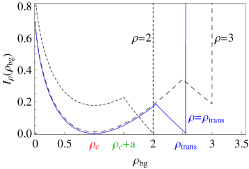
Figure 4: The rate function $I_{\rho}(\rho_{bg})$ for $c_{0}=2$, $c_{1}=1$, $a=0.5$ and various values of $\rho$. For $\rho>\rho_{c}+a$ the function has a local minimum at $\rho_{bg}=\rho_{c}$, which becomes the global minimum for $\rho>\rho_{trans}$.

Figure 4 shows that the distribution of $\Sigma_{L}^{bg}$ concentrates on values of the order $\rho L$ for $\rho<\rho_{trans}$ and on values of the order $\rho_{c}L$ for $\rho>\rho_{trans}$. These two cases correspond to the phases $F/C$ and $C/F$, respectively, and have been identified already in the previous section. But in Figure 4 also the role of $\rho_{c}+a$ can be identified. For $\rho<\rho_{c}+a$, the rate function $I_{\rho}(\rho_{bg})$ (128) has only one minimum $I_{\rho}(\rho)=0$, whereas for $\rho>\rho_{c}+a$ it has an additional local minimum at $\rho_{bg}=\rho_{c}$, i.e. the condensed phase becomes metastable. For $\rho>\rho_{trans}$ this local minimum becomes the global one, and the fluid phase becomes metastable. For $\rho=\rho_{trans}$ the rate function vanishes for both phases, but the finer analysis of Theorem 2 reveals that the fluid phase is already metastable in this case.

By definition, the observable $\Sigma_{L}^{bg}({\boldsymbol{\eta}})$ changes at most by $\pm 1$ during each jump of a particle. So the process $\big{(}\Sigma_{L}^{bg}({\boldsymbol{\eta}}(t))\big{)}_{t\geq 0}$ is a one-dimensional simple random walk (or a birth-death process) on $\{0,1,\ldots,N\}$, whose stationary large deviation rate function is $I_{\rho}$. The minima of this rate function correspond to the fluid phase for $\rho_{bg}=\rho$ and the condensed phase for $\rho_{bg}=\rho_{c}$. For finite $L$ the system has two quasi-stationary distributions

$$\pi_{L,N}(.|X_{L,N}^{0})\quad\mbox{and}\quad\pi_{L,N}(.|X_{L,N}^{1})\ ,$$ (145)

corresponding to the fluid and the condensed phase, respectively. Analogous to (105) we define

$$\tilde{\pi}_{L,N}=\pi_{L,N}(.|X_{L,N}^{1},\,L\in\mathrm{argmax})^{1,..,L-1}$$ (146)

Proposition 3

In the limit $L\to\infty$, $N/L\to\rho$, we have for all $\rho\geq 0$

$$h\big{(}\pi_{L,N}(.|X_{L,N}^{0}),\nu^{L}_{\phi_{\infty}(\rho),\infty}\big{)}\to 0\quad\mbox{and}\quad\pi_{L,N}(.|X_{L,N}^{0})\to\nu_{\phi_{\infty}(\rho),\infty}\ ,$$ (147)

and for all $\rho\geq\rho_{c}+a$

$$H\big{(}\tilde{\pi}_{L,N},\nu^{L-1}_{c_{1},\infty}\big{)}\to 0\quad\mbox{and}\quad\pi_{L,N}(.|X_{L,N}^{1})\to\nu_{c_{1},\infty}\ .$$ (148)

In both cases the second convergence is weakly with respect to bounded cylinder test functions.

As in Theorem 4, we can show convergence in total relative entropy (148) for the condensed phase, which is much stronger than convergence in specific relative entropy (see comments in the previous section).

Proof. The first statements in (147) and (148) can be proved analogous to Theorem 3 and Theorem 4, respectively. Since

$$\pi_{L,N}({\boldsymbol{\eta}}|X_{L,N}^{0})=\frac{\pi_{L,N}({\boldsymbol{\eta}})}{\pi_{L,N}(X_{L,N}^{0})}{\mathbbm{1}}_{X_{L,N}^{0}}({\boldsymbol{\eta}})=\frac{1}{|X_{L,N}^{0}|}{\mathbbm{1}}_{X_{L,N}^{0}}({\boldsymbol{\eta}})$$ (149)

is the uniform measure on $X_{L,N}^{0}$, we get for (147) analogous to (97)

$$h\big{(}\pi_{L,N}(.|X_{L,N}^{0}),\nu_{\phi_{\infty}(\rho),\infty}^{L}\big{)}=$$ (150)

$$\qquad=\frac{1}{L}\sum_{{\boldsymbol{\eta}}\in X_{L,N}^{0}}\pi_{L,N}({\boldsymbol{\eta}}|X_{L,N}^{0})\log\frac{z_{\infty}\big{(}\phi_{\infty}(\rho)\big{)}^{L}}{\big{(}\phi_{\infty}(\rho)/c_{0}\big{)}^{N}|X_{L,N}^{0}|}=$$

$$\qquad=p_{fluid}\big{(}\phi_{\infty}(\rho)\big{)}-\frac{N}{L}\,\log\frac{\phi_{\infty}(\rho)}{c_{0}}-\frac{1}{L}\,\log|X_{L,N}^{0}|$$

$$\qquad\to s_{fluid}(\rho)+\rho\log c_{0}-\chi(\rho)=0\quad\mbox{as }L\to\infty$$

for all $\rho\geq 0$, using Lemma 1. Note that here we are a priori restricted to $X_{L,N}^{0}$ so that there is no error term as in (97).
The same holds for a modification of (112) to derive (148). Using

$$\tilde{\pi}_{L,N}(\hat{\boldsymbol{\eta}}) = \frac{\pi_{L,N}(\hat{\boldsymbol{\eta}},N-\Sigma_{L-1}(\hat{\boldsymbol{\eta}}))}{\pi_{L,N}(\mathrm{argmax}=L,X_{L,N}^{1})}\,{\mathbbm{1}}_{\mathrm{argmax}=L,X_{L,N}^{1}}\big{(}\hat{\boldsymbol{\eta}},N{-}\Sigma_{L{-}1}(\hat{\boldsymbol{\eta}})\big{)}=$$ (151)

$$= \frac{L(c_{0}/c_{1})^{{-}\Sigma_{L-1}(\hat{\boldsymbol{\eta}})-R}c_{1}^{-N}}{\pi_{L,N}(X_{L,N}^{1})\,Z_{L,N}}{\mathbbm{1}}_{\mathrm{argmax}=L,X_{L,N}^{1}}\big{(}\hat{\boldsymbol{\eta}},N{-}\Sigma_{L{-}1}(\hat{\boldsymbol{\eta}})\big{)}$$

and $\pi_{L,N}(X_{L,N}^{1})\to 1$, we get in direct analogy to the proof of Theorem 4

$$H(\tilde{\pi}_{L,N},\nu_{c_{1},\infty}^{L-1}) = \sum_{\hat{\boldsymbol{\eta}}\in\hat{X}_{L-1}^{0}}\tilde{\pi}_{L,N}(\hat{\boldsymbol{\eta}})\log\frac{L\,(c_{0}/c_{1})^{-R}\,c_{1}^{-N}z_{\infty}(c_{1})^{L{-}1}}{\pi_{L,N}(X_{L,N}^{1})\,Z_{L,N}}=$$ (152)

$$= \pi_{L,N}(X_{L,N}^{1})\log\big{(}1+o(1)\big{)}\to 0\quad\mbox{as }L\to\infty\ .$$

The second statements in (147) and (148) follow completely analogously to the proofs of Theorem 3 and Theorem 4. $\Box$

With Theorems 3 and 4 both statements of Proposition 3 follow directly from Corollary 1 and Theorem 2, but only for $\rho<\rho_{trans}$ and $\rho\geq\rho_{trans}$, respectively, where the quasi-stationary distributions converge to the stationary distribution.

For finite $L$, both phases have life-times of the order $\sim e^{\xi(\rho)L}$ exponential in the system size for all $\rho>\rho_{c}+a$, where the exponential rate $\xi(\rho)$ depends on the density. It can be calculated using the hitting times

$$\tau_{L}^{fluid}(\rho) := \inf\big{\{}t\geq 0\,\big{|}\,\max_{x\in\Lambda_{L}}\eta_{x}(t)>R\big{\}}\ ,$$

$$\tau_{L}^{cond}(\rho) := \inf\big{\{}t\geq 0\,\big{|}\,\max_{x\in\Lambda_{L}}\eta_{x}(t)\leq R\big{\}}\ ,$$ (153)

which depend on the initial configuration as well as the time evolution. Due to the effective one-dimensional random walk picture mentioned above, the quasi-stationary expectations of these random variables are determined by the rate functions at the locations of local minima and maxima. These are

$$I_{\rho}(\rho) = s_{can}(\rho)-s_{fluid}(\rho)\qquad\qquad\qquad\qquad\qquad\qquad\ \mbox{(min.)}$$

$$I_{\rho}(\rho-a) = s_{can}(\rho)-s_{fluid}(\rho-a)+a\log c_{0}\qquad\qquad\qquad\ \mbox{(max.)}$$

$$I_{\rho}(\rho_{c}) = s_{can}(\rho)-s_{fluid}(\rho_{c})+a\log\frac{c_{0}}{c_{1}}+(\rho-\rho_{c})\log c_{1}\,\,\mbox{(min.)}\,,$$ (154)

where the last two are only defined for $\rho>\rho_{c}+a$ (cf. Figure 4). Note that $I_{\rho}(\rho)=0$ for $\rho\leq\rho_{c}$, whereas $I_{\rho}(\rho_{c})=0$ for $\rho\geq\rho_{c}$. For $\rho>\rho_{c}+a$ we then have

$$\xi^{fluid}(\rho) := \lim_{L\to\infty}\frac{1}{L}\log\ll\tau_{L}^{fluid}(\rho)\gg_{\pi_{L,N}(.|X_{L,N}^{0}),e^{\mathcal{L}t}}=I_{\rho}(\rho-a)-I_{\rho}(\rho)=$$

$$= s_{fluid}(\rho)-s_{fluid}(\rho-a)+a\log c_{0}\ ,$$

$$\xi^{cond}(\rho) := \lim_{L\to\infty}\frac{1}{L}\log\ll\tau_{L}^{cond}(\rho)\gg_{\pi_{L,N}(.|X_{L,N}^{1}),e^{\mathcal{L}t}}=I_{\rho}(\rho-a)-I_{\rho}(\rho_{c})=$$ (155)

$$= s_{fluid}(\rho_{c})-s_{fluid}(\rho-a)+(\rho_{c}+a-\rho)\log c_{1}$$

where $\ll..\gg_{\pi_{L,N}(.|X_{L,N}^{0}),e^{\mathcal{L}t}}$ denotes the average with respect to a quasi-stationary initial distribution and the time evolution given by the generator $\mathcal{L}$ (6). Note that for $\rho<\rho_{c}+a$, $\xi_{fluid}(\rho)=\infty$ and $\xi_{cond}(\rho)$ is not defined, since the condensed phase is not stable. The asymptotic behaviour as $\rho\to\infty$ is given by

$$\xi^{fluid}(\rho) \simeq \log\frac{1+\rho}{1+\rho-a}\to 0$$

$$\xi^{cond}(\rho) \simeq \rho\log\frac{c_{0}}{c_{1}}-\log(1+\rho-a)+const.\to\infty\ .$$ (156)

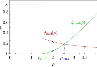
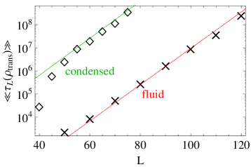
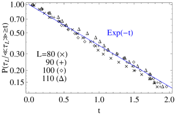
Figure 5: Life-times of fluid and condensed phase for $c_{0}=2$, $c_{1}=1$, $a=0.5$.
Top: The exponential rate $\xi(\rho)$ of the life-time as a function of the density. $\times$ and $\diamond$ denote Monte Carlo data, errors are of the size of the symbols. Bottom left: Expected life-times as used in (5) in a logarithmic plot as a function of $L$ for $\rho=\rho_{trans}$. Bottom right: Tail distribution of the normalized lifetimes $\tau_{L}^{cond}(\rho_{trans})/\ll\tau_{L}^{cond}(\rho_{trans})\gg$, compared with the tail of an $\mathit{Exp}(1)$ random variable.

For all $a>0$ we have $\xi^{fluid}(\rho_{c}+a)>0=\xi^{cond}(\rho_{c}+a)$ and $\xi^{fluid}(\rho_{trans})=\xi^{cond}(\rho_{trans})$, as expected. This behaviour is illustrated in Figure 5 for some specific values of the parameters. The predictions are in very good agreement with data from Monte Carlo simulations, a few of which are presented in the figure. On the bottom left for $\rho=\rho_{trans}$ we see that the expected lifetimes for the condensed phase are larger than for the fluid phase, which is in accordance with Theorem 2. There appears to be a polynomial correction in the condensed phase, but the data are not good enough to measure the power in $L$.

Note that the last part of the derivation in this section is not rigorous, since strictly speaking $\big{(}\Sigma_{L}^{bg}({\boldsymbol{\eta}}(t))\big{)}_{t\geq 0}$ is not a Markov process. Still one could use a potential theoretic approach analogous to [3], to show rigorously that the average life times of both phases are exponential in $L$. However, getting the right timescale with this approach would require quite some technical effort. Besides the exponential growth rate of the life times with the system size $L$, simulations also indicate that the distribution of the lifetimes is actually exponential, as can be seen in Figure 5 on the bottom right. This is to be expected, since the system effectively jumps between the two metastable phases in a Markovian way.

6 Dependence on the number of particles

In this section we consider the case where the jump rates depend on the number of particles in the system rather than the lattice size, which is also the case in some models for granular clustering [23, 4], one of our main motivations for this study. We modify our original model (4),

$$g_{R}(k)=\left\{\begin{array}[]{cl}c_{0}&,\ k\leq R\\ c_{1}&,\ k>R\end{array}\right.\quad\mbox{for }k\geq 1\ ,\quad g(0)=0\ ,$$ (159)

where $R$ is now a function of the number of particles $\Sigma_{L}({\boldsymbol{\eta}})$. For simplicity we concentrate on the specific choice $R=a\,\Sigma_{L}({\boldsymbol{\eta}})$ with $a\in[0,1)$, since $a\geq 1$ is not interesting for this model. So in principle, the jump rates do not only depend on the local occupation number but on the global configuration. But restricted to a subset $X_{L,N}$ with fixed particle number $\Sigma_{L}({\boldsymbol{\eta}})=N$, $R$ is just a parameter, the process is well defined and standard results on stationary measures apply. Therefore the canonical measures are well defined as in (42). In particular, Theorems 1 to 4 still hold and the proofs apply directly, where $a$ should be replaced by $a\rho$, since now $R/L\to\rho\,a$. So analogous to (51) the transition density $\rho_{trans}$ is determined by the relation

$$a=\Big{(}s_{fluid}(\rho_{c})-(\rho-\rho_{c})\log c_{1}-s_{fluid}(\rho)\Big{)}\Big{/}\Big{(}\rho\log\frac{c_{0}}{c_{1}}\Big{)}\ ,$$ (160)

and $s_{fluid}$ is given as in (34). The canonical entropy density $s_{can}$ is still given by (49), but the contribution of the condensate, which determines the behaviour for large $\rho$, is now given by

$$s_{cond}(\rho,\rho_{c})=-\rho\Big{(}a\log\frac{c_{0}}{c_{1}}+\log c_{1}\Big{)}+\rho_{c}\log c_{1}\ .$$ (161)

This leads to

$$s_{can}(\rho)=\left\{\begin{array}[]{cl}s_{fluid}(\rho)&,\ \rho\leq\rho_{trans}\\ s_{fluid}(\rho_{c}){-}\rho\Big{(}a\log\frac{c_{0}}{c_{1}}{+}\log c_{1}\Big{)}{+}\rho_{c}\log c_{1}&,\ \rho>\rho_{trans}\end{array}\right..$$ (164)

To study the equivalence of ensembles, one has to define the grand-canonical measures. This is not as straightforward as in (12), since the number of particles $\Sigma_{L}({\boldsymbol{\eta}})$ and thus $R$ is now a random variable. However, we know that the set of all stationary measures is convex, and the extremal points are the canonical measures (see e.g. [22] or [16]). So the grand-canonical measures can be defined as convex combinations of canonical measures,

$$\nu^{L}_{\phi,R}({\boldsymbol{\eta}})=\prod_{x\in\Lambda_{L}}w_{R}^{L}(\eta_{x})\,\phi^{\eta_{x}}\Big{/}\sum_{N=0}^{\infty}\phi^{N}Z_{L,N}\ .$$ (165)

If the weights $w_{R}(k)$ depended only on the system size $L$, this would be equivalent to (12), but here the measures are obviously not of product form since the weights depend on the total number of particles through $R=a\Sigma_{L}({\boldsymbol{\eta}})$. Also the normalizing partition function

$$Z_{R}(\phi):=\sum_{N=0}^{\infty}\phi^{N}Z_{L,N}$$ (166)

does not factorize, since now $Z_{L,N}=w_{aN}^{L}(X_{L,N})$. Nevertheless we can define the pressure

$$p_{gcan}(\phi):=\lim_{L\to\infty}\frac{1}{L}\log\sum_{N=0}^{\infty}\phi^{N}Z_{L,N}\ ,$$ (167)

and by a saddle point argument analogous to the proof of Theorem 1 this is well defined and given by

$$p_{gcan}(\phi)=\sup_{\rho\geq 0}\big{(}\rho\log\phi+s_{can}(\rho)\big{)}\ ,$$ (168)

the Legendre transform of the negative canonical entropy density (164). With (161) we have for $\rho>\rho_{trans}$

$$\rho\log\phi+s_{can}(\rho)=\rho\Big{(}\log\phi-a\log\frac{c_{0}}{c_{1}}-\log c_{1}\Big{)}+\rho_{c}\log c_{1}\ ,$$ (169)

which, analogously to (37), implies

$$p_{gcan}(\phi)=\left\{\begin{array}[]{cl}p_{fluid}(\phi)&,\ \phi<\phi_{c}(a)\\ \infty&,\ \phi\geq\phi_{c}(a)\end{array}\right.\ .$$ (172)

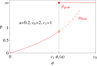
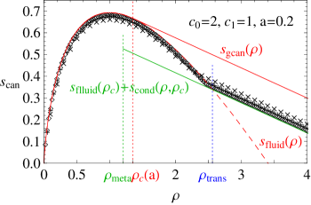
Figure 6: Pressure and entropies for $a=0.2$, $c_{0}=2$ and $c_{1}=1$ as given in (172), (164) and (177). Data points are calculated numerically according to (81) with $L=100\ (\times)$, $200\ (+)$, $400\ (\Diamond)$, and show good agreement with the theoretical predictions for the thermodynamic limit.

The difference is that now the pressure is finite up to

$$\phi_{c}(a):=c_{1}\Big{(}\frac{c_{0}}{c_{1}}\Big{)}^{a}\geq c_{1}\ ,$$ (173)

which is strictly bigger than the value $c_{1}$ in (37) for all $a\in(0,1)$. Note that for $\phi=\phi_{c}(a)$ the saddle point argument (168) does not apply and (167) diverges, so $p_{gcan}\big{(}\phi_{c}(a)\big{)}=\infty$, see Figure 6 left. As a consequence of (172), the critical density defined as in (18) is now $a$-dependent and given by

$$\rho_{c}(a):=\rho_{\infty}\big{(}\phi_{c}(a)\big{)}=\frac{c_{1}^{1-a}}{c_{0}^{1-a}-c_{1}^{1-a}}\ ,$$ (174)

where $\rho_{\infty}$ is still given by (16). So analogous to (40), the grand-canonical entropy density is given by the negative Legendre transform of (172),

$$s_{gcan}(\rho)=\left\{\begin{array}[]{cl}s_{fluid}(\rho)&,\ \rho\leq\rho_{c}(a)\\ s_{fluid}(\rho_{c}(a))-(\rho-\rho_{c}(a))\log\phi_{c}(a)&,\ \rho>\rho_{c}(a)\end{array}\right.\ .$$ (177)

By definition, this is again the concave hull of $s_{can}(\rho)$, as can be seen in Figure 6, right. The canonical entropy density is calculated numerically using (81) for different values of $L$ and $N$, and as before the results agree very well with the predictions.

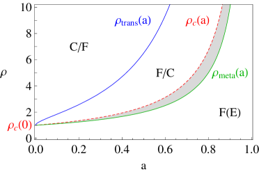
Figure 7: Stationary phase diagram of the process (159) for $c_{0}=2$, $c_{1}=1$. The phases $F(E)$, $F/C$ and $C/F$ are defined in Section 2, $F(E)$ and $F/C$ overlap (shaded region) and phase $F$ is empty.

As in the original model, the case $a=0$ leads to a continuous phase transition and this line of the phase diagram is identical to Figure 1. But for all $a\in(0,1)$, $\rho_{c}(a)>\rho_{c}(0)$, which is the value in (18) for the original model. So the phase region $F(E)$ in the phase diagram is larger than in the original model (see Figure 7). To complete the phase diagram, we have to derive the analogue of the transition line $\rho_{c}+a$, which we call $\rho_{meta}$ in the following. This is defined by the emergence of a metastable condensed phase, characterized by a second local maximum of the rate function $I_{\rho}(\rho_{bg})$ in Theorem 5. The proof of this theorem makes use of the grand-canonical measures, and since these are now of different form, it does not apply directly. However, with some effort the proof can be written purely in terms of canonical measures (not shown here), and so the result (131) still applies, of course with $a$ replaced by $\rho\,a$. An analysis similar to Section 5 reveals that the rate function has an additional local minimum

$$I_{\rho}\big{(}\rho_{c}(0)\big{)}\quad\mbox{for }\rho>\rho_{meta}=\frac{\rho_{c}(0)}{1-a}\ .$$ (178)

So there exists a metastable condensed phase with background density $\rho_{c}(0)$, which is still the same as in the previous model, independent of $a$. This is to be expected, since the outflow of the condensate site has to match the background current. A simple heuristic argument along these lines provides a general framework to understand the transition, and is presented in detail in [18]. Note that in comparison with (174),

$$\rho_{meta}(a)\leq\rho_{c}(a)\quad\mbox{for all }a\in[0,1)\ ,$$ (179)

with equality if and only if $a=0$. This follows immediately from the elementary inequality $x^{1-a}-1\leq(1-a)(x-1)$. So the phase regions $F(E)$ and $F/C$ as defined in Section 2 overlap (see shaded region in Figure 7), and the region $F$ is empty. In contrast to our previous model, the equivalence of ensembles still holds in the presence of a metastable condensed phase.

7 Discussion

7.1 Differences to previous results

In the following we discuss differences in the condensation transition between zero-range processes with and without size-dependence in the jump rates. To simplify matters we concentrate on the rates (4) for $L$-dependent jump rates, but the features we discuss should hold in general.

• Without $L$-dependence the condensation transition in zero-range processes is continuous, i.e. the background density $\rho_{bg}$ is a continuous function of the total particle density $\rho$. For model (4) this is only true if $a=0$, for $a>0$ the background density $\rho_{bg}=\rho_{c}<\rho_{trans}$ is smaller than the transition density and the transition is discontinuous.

• If the jump rates do not depend on $L$, the equivalence of ensembles holds for all densities, and for $\rho\geq\rho_{c}$ the entropy density is linear in $\rho$ which is often characterized as partial equivalence of ensembles [8, 31]. The reason is that the contribution of the condensate to the entropy density vanishes as $L\to\infty$. In model (4) this contribution does not vanish, cf. Theorem 1, and therefore we have only equivalence of ensembles for $\rho\leq\rho_{c}$ and nonequivalence for larger densities. As a consequence of this, the canonical entropy density is non-concave, whereas it is concave in case of no $L$-dependence.

• Another striking feature of model (4) is that it exhibits ergodicity breaking, i.e. for $\rho>\rho_{c}+a$ there are two phases, fluid and condensed, with life-times exponential in $L$, one of which is metastable depending on the density. Without $L$-dependence in the jump rates this does not occur, and for all densities there is only one stable phase, either fluid for $\rho\leq\rho_{c}$ or condensed for $\rho>\rho_{c}$.

So far a discontinuous transition in a zero-range process has only been observed heuristically in a two-species system where the stationary state is not known [15]. The above features only concern the stationary measure, and for systems without $L$-dependence they have been shown rigorously in a general context [16]. In the following we comment on further differences regarding equilibration and stationary dynamics, which have been studied only heuristically so far.

• If we prepare a system without $L$-dependence in a homogeneous distribution with density $\rho>\rho_{c}$ it exhibits coarsening [17, 13]. Initially, clusters form all over the lattice, and as time progresses the larger cluster sites gain particles on the expense of the smaller cluster, leading to a self-similar time evolution. The driving force for this behaviour is the fact that there is no stable fluid phase with density $\rho>\rho_{c}$. This is not the case in model (4), which does not exhibit coarsening for that reason. Instead, it takes a time of order $e^{\xi^{fluid}L}$ before the condensate appears.

• In a similar setting metastability has been reported as a precursor of the coarsening regime, i.e. before coarsening to a single condensate sets in [20]. Unlike in the present case, heuristic theoretical analysis supported by Monte-Carlo simulation shows that the life time of these metastable configurations does not grow exponentially with system size.

• For systems without $L$-dependence, in the condensed phase the distribution of the homogeneous background has a sub-exponential tail [16]. In connection to this, the stationary time scale for movement of the condensate location (once a single condensate has build up) is also sub-exponential in $L$, as was found heuristically in [14] in case of a power law. For model (4) the background distribution is just $\nu_{c_{1},\infty}^{1}(k)\sim(c_{1}/c_{0})^{-k}$ (see Theorem 4), which has an exponential tail. Therefore condensates can move only by dissolving completely and, after a time of order $e^{\xi^{fluid}L}$ in the coexisting fluid phase, forming on a different site. So the time scale for the stationary motion of a condensate is exponential in the system size.

The long time it takes to form a condensate in the present model is observed in Monte Carlo simulations and is explained heuristically by a random walk picture in Section 5. The time it takes for the transition between the phases depends on the specific model as well as the definition of the phases. In any case its order is subexponential in the system size, and for the model (4) it is actually of order $L$. Moreover, if $\rho>\rho_{c}+na$ for $n\geq 1$ also more than one condensate is possible. But as can be seen in the proof of Theorem 1, the contribution to the partition function of such a configuration is negligible. Therefore one typically observes only one condensate, which is a common feature with the stationary behaviour of a system without $L$-dependence, although both cases have very different life times. In [27] a hydrodynamic theory is developed for the time evolution under Eulerian scaling above the condensation threshold. This leads to a generic picture for the evolution of a space-dependent initial density profile with total supercritical density in systems with rates that do not depend on $L$. It would be interesting to study this problem in the present model.

Finally, we would also like to stress an intriguing difference to the usual theory of first order phase transitions in statistical mechanics. In systems with finite local state space or with bounded Hamiltonians, such as spin systems (Ising model) or exclusion models, the pressure $p$ is defined for all fugacities $\phi\geq 0$, and a first order phase transition is a result of the pressure being non-analytic (see e.g. [25, 35]). In the model we studied here, the pressure (37) is defined only for $\phi<c_{1}$, but is analytic on its domain. Therefore the phase transition is a result of this bounded domain in connection with the conservation of the particle number, and cannot be understood by studying the grand-canonical measures alone. This is in contrast to previously studied systems without $L$-dependent jump rates, where the presence of condensation can be characterized by a closed domain of the pressure $p$ (cf. [16]).

7.2 Summary

In this paper we presented a rigorous analysis of a discontinuous phase transition in a simple zero-range process with size-dependent jump rates. The model acts as a prototype for systems with that feature and the results are expected to be qualitatively similar for a large class of models. This will be discussed in detail in a forthcoming publication [18]. Going beyond earlier heuristic discussions of the phase transition in terms of the order parameter [23, 4, 7], our analysis provides a detailed picture of the phase transition in terms of the entire ensemble. In particular we note that our approach is a pure equilibrium description, based as in the work of [23, 4] on the notion of thermally activated processes. Hence there is no need for an appeal [7] to a non-equilibrium dissipative structure, maintained by a flux of entropy, for understanding the nature of the condensation transition in the granular shaking experiment.

Since our results only concern the stationary distribution they do not depend on the geometry or dimension of the lattice. The model shows the same features observed in granular clustering, namely metastability and a first order transition. The only difference is that there is no region in the phase diagram where the fluid phase becomes unstable. This is due to the simple choice of rates in this first analysis, and the issue will be addressed in [18].

Appendix

A.3 Proof of Proposition 2

For $\rho<\rho_{c}$ (32) follows by standard results and for $\rho>\rho_{c}$ we have as $L\to\infty$

$$\nu^{1}_{\phi_{R}(\rho),R}(\eta_{x}^{L}>R)\simeq\sqrt{\frac{\rho-\rho_{c}}{z_{\infty}(c_{1})}}\Big{(}\frac{c_{1}}{c_{0}}\Big{)}^{R/2}\ .$$ (180)

Therefore if we define the truncated occupation numbers $\hat{\eta}_{x}^{L}=\eta_{x}^{L}\wedge R$, we have

$$\nu^{L}_{\phi_{R}(\rho),R}\Big{(}\frac{1}{L}\sum_{x\in\Lambda_{L}}(\eta_{x}^{L}-\hat{\eta}_{x}^{L})\neq 0\Big{)}=\nu^{L}_{\phi_{R}(\rho),R}\big{(}\mbox{at least one }\eta_{x}^{L}>R\big{)}=$$ (181)

$$\quad=1-\Big{(}1-\nu^{1}_{\phi_{R}(\rho),R}(\eta_{x}>R)\Big{)}^{L}\leq CL\Big{(}\frac{c_{1}}{c_{0}}\Big{)}^{R/2}\ .$$

With $R\gg\log L$ this bound is summable and the Borel-Cantelli Lemma implies that

$$\frac{1}{L}\sum_{x\in\Lambda_{L}}\eta_{x}^{L}-\frac{1}{L}\sum_{x\in\Lambda_{L}}\hat{\eta}_{x}^{L}\to 0\quad a.s.\quad\mbox{as }L\to\infty.$$ (182)

Moreover $\langle\hat{\eta}_{x}\rangle=\rho_{c}+O\big{(}(\frac{c_{1}}{c_{0}})^{R/2}\big{)}$ and $Var(\hat{\eta}_{x})\leq\frac{c_{0}c_{1}}{(c_{0}-c_{1})^{2}}+O\big{(}R(\frac{c_{1}}{c_{0}})^{R/2}\big{)}$ and therefore by the usual strong law we have $\sum_{x\in\Lambda_{L}}\hat{\eta}_{x}^{L}\to\rho_{c}\quad a.s.$ .
Taken together, this implies (32) for $\rho>\rho_{c}$, and $\rho=\rho_{c}$ works analogously with the power $R/2$ replaced by $R/4$.

A.4 Proof of Lemma 1

Each configuration in $X_{L,N}\setminus X^{0}_{L,N}$ has at least one site with more than $R$ particles and we denote the number of such sites by

$$E({\boldsymbol{\eta}}):=\sum_{x\in\Lambda_{L}}{\mathbbm{1}}_{\eta_{x}>R}({\boldsymbol{\eta}})\ .$$ (183)

Note that for ${\boldsymbol{\eta}}\in X_{L,N}\setminus X^{0}_{L,N}$ we have

$$1\leq E({\boldsymbol{\eta}})\leq M=\lceil N/R\rceil\ ,$$ (184)

where $M$ is as defined in (45). For each configuration we define

$$S({\boldsymbol{\eta}}):=\big{(}\eta_{x}\wedge R\,\big{|}\,x{\in}\Lambda_{L}\big{)}\cup\big{(}\eta_{x}{-}R\,\big{|}\,x{\in}\Lambda_{L},\,\eta_{x}{>}R\big{)}\in X_{L{+}E({\boldsymbol{\eta}}),N}\ .$$ (185)

If $E\big{(}S({\boldsymbol{\eta}})\big{)}>0$, we have to repeat this mapping at most $M$ times such that

$$\bar{\boldsymbol{\eta}}:=S^{M}({\boldsymbol{\eta}})\in X_{L+l({\boldsymbol{\eta}}),N}^{0}\ ,$$ (186)

where $l({\boldsymbol{\eta}})\leq M$ denotes the total number of extra coordinates. For $l({\boldsymbol{\eta}})<M$ we can identify $\bar{\boldsymbol{\eta}}$ by a configuration in $X_{L+M,N}^{0}$, by setting all remaining coordinates equal to zero. By this construction it is clear that for each ${\boldsymbol{\eta}}\in X_{L,N}\setminus X^{0}_{L,N}$ there exists a unique $\bar{\boldsymbol{\eta}}\in X_{L+M,N}^{0}$, i.e.

$$\big{|}X_{L,N}\setminus X^{0}_{L,N}\big{|}=\big{|}X_{L,N}\big{|}-\big{|}X^{0}_{L,N}\big{|}\leq\big{|}X_{L+M,N}^{0}\big{|}\ .$$ (187)

Further, each $\bar{\boldsymbol{\eta}}$ has the special property that at least $l({\boldsymbol{\eta}})$ sites contain exactly $R$ particles, and there are only $L$ sites whose occupation number can be less or equal than that. Therefore we can improve the above estimate as

$$\big{|}X_{L,N}\big{|}-\big{|}X^{0}_{L,N}\big{|}\leq{L+M\choose M}\,\big{|}X_{L,N-R}^{0}\big{|}\leq{L+M\choose M}\,\frac{\big{|}X_{L,N}^{0}\big{|}}{(L-M)^{R}}\ ,$$ (188)

where the combinatorial factor counts the number of positions of sites with $R$ particles. We also used the fact that for all $k=1,\ldots,R$

$$\big{|}X_{L,N-k+1}^{0}\big{|}\geq(L-M)\big{|}X_{L,N-k}^{0}\big{|}\ ,$$ (189)

since there are at least $L-M$ positions to put an additional particle without violating the constraint $\eta_{x}\leq R$ for all $x$. Together with the obvious fact that $\big{|}X^{0}_{L,N}\big{|}\leq\big{|}X_{L,N}\big{|}$, this proves the first statement of the lemma, i.e.

$$\frac{1}{1+{L+M\choose M}\big{/}(L-M)^{R}}\,\big{|}X_{L,N}\big{|}\leq\big{|}X^{0}_{L,N}\big{|}\leq\big{|}X_{L,N}\big{|}\ .$$ (190)

With Stirling’s formula we get

$$\lim_{L\to\infty}\frac{1}{L}\log{L{+}M\choose L}=\lim_{L\to\infty}\Big{(}\big{(}1{+}\tfrac{M}{L}\big{)}\log\big{(}1{+}\tfrac{M}{L}\big{)}{-}\tfrac{M}{L}\log\tfrac{M}{L}\Big{)}=0\ .$$ (191)

since $M/L\to 0$ as $L\to\infty$. Therefore

$$\frac{1}{L}\log\frac{1}{1+{L+M\choose M}\big{/}(L-M)^{R}}\to 0$$ (192)

and (190) certainly includes the second statement of the lemma. More detailed, we get to leading order as $L\to\infty$, $N/L\to\rho$,

$$\frac{{L+M\choose M}}{(L-M)^{R}}=\Big{(}\frac{R+\rho}{\rho}\Big{)}^{\rho L/R+1/2}\Big{(}1+\frac{\rho}{R}\Big{)}^{L}\frac{L^{-R-1/2}}{\sqrt{2\pi}}\big{(}1+o(1)\big{)}\ .$$ (193)

This vanishes for all $\rho\geq 0$ if

$$R\log L-\frac{\rho L}{R}\log R\gg\log R\vee\frac{\rho L}{R}\quad\mbox{as }L\to\infty\ ,$$ (194)

which is certainly the case for $R\gg\sqrt{L}$. $\Box$

References

- [1] Andjel, E.: Invariant measures for the zero range process. Ann. Probab. 10(3), 525–547 (1982)
- [2] Angel, A.G., Evans, M.R., Levine, E., Mukamel, D.: Criticality and Condensation in a Non-Conserving Zero Range Process. J. Stat. Mech. P08017 (2007)
- [3] Bovier, A.: Metastability: a potential theoretic approach. In: Proceedings of the ICM 2006, Madrid, pp. 499–518, European Mathematical Society (2006)
- [4] Coppex, F., Droz, M., Lipowski, A.: Dynamics of the breakdown of granular clusters. Phys. Rev. E 66, 011305 (2002)
- [5] Csiszár, I.: I-divergence geometry of probability distributions and minimization problems. Ann. Probab. 3(1), 146- 158 (1975)
- [6] Csiszár, I.: Sanov property, generalized i-projection and a conditional limit theorem. Ann. Probab. 12, 768–793 (1984)
- [7] Eggers, J.: Sand as Maxwell’s Demon. Phys. Rev. Lett. 83(25), 5322-5325 (1999)
- [8] Ellis, R.S., Haven, K., Turkington, B.: Large deviation principles and complete equivalence and nonequivalence results for pure and mixed ensembles. J. Stat. Phys. 101, 999–1064 (2000)
- [9] Evans, M.R.: Phase transitions in one-dimensional nonequilibrium systems. Braz. J. Phys. 30(1), 42–57 (2000)
- [10] Evans, M.R., Hanney, T.: Nonequilibrium statistical mechanics of the zero-range process and related models. J. Phys. A: Math. Gen. 38, R195–R239 (2005)
- [11] Evans, M.R., Hanney, T., Majumdar, S.N.: Interaction driven real-space condensation. Phys. Rev. Lett. 97, 010602 (2006)
- [12] Ferrari, P.A., Landim, C., Sisko, V.V.: Condensation for a fixed number of independent random variables. J. Stat. Phys. 128, 1153-1158 (2007)
- [13] Godrèche, C.: Dynamics of condensation in zero-range processes. J. Phys. A: Math. Gen. 36, 6313-6328 (2003)
- [14] Godrèche, C., Luck, J.M.: Dynamics of the condensate in zero-range processes. J. Phys. A: Math. Gen. 38, 7215-7237 (2005)
- [15] Godrèche, C.: Nonequilibrium phase transition in a non integrable zero-range process. J. Phys. A: Math. Gen. 39, 9055–9069 (2006)
- [16] Grosskinsky, S.: Equivalence of ensembles for two-component zero-range invariant measures. accepted in Stoch. Proc. Appl. (DOI: 10.1016/j.spa.2007.09.006)
- [17] Grosskinsky, S., Schütz, G.M., Spohn, H.: Condensation in the zero range process: stationary and dynamical properties. J. Stat. Phys. 113(3/4), 389–410 (2003)
- [18] Grosskinsky, S., Schütz, G.M.: in preparation
- [19] Kafri, Y., Levine, E., Mukamel, D., Schütz, G.M., Török, J.: Criterion for phase separation in one-dimensional driven systems. Phys. Rev. Lett. 89(3), 035702 (2002)
- [20] Kaupuzs, J., Mahnke, R., Harris, R.J.: Zero-range model of traffic flow. Phys. Rev. E 72(5), 056125 (2005)
- [21] Levine, E., Mukamel, D., Schütz, G.M.: Zero range process with open boudaries. J. Stat. Phys. 120(5/6), 759-778 (2002)
- [22] Liggett, T.M.: Interacting Particle Systems. Springer, Berlin (2004)
- [23] Lipowski, A., Droz, M.: Urn model of separation of sand. Phys. Rev. E 65, 031307 (2002)
- [24] Loulakis, M., Armendáriz, I.: Thermodynamic Limit for the Invariant Measures in Supercritical Zero Range Processes. arXiv:0801.2511 (2008)
- [25] Ruelle, D.: Statistical mechanics: rigorous results. W.A. Benjamin, New York-Amsterdam (1969)
- [26] Schlichting, H.J., Nordmeier, V.: Strukturen im Sand. Kollektives Verhalten und Selbstorganisation bei Granulaten. Math. naturw. Unterricht 496, 323-332 (1996) (in German)
- [27] Schütz, G.M., Harris, R.J.: Hydrodynamics of the zero-range process in the condensation regime. J. Stat. Phys. 127(2), 419-430 (2007)
- [28] Schwarzkopf, Y., Evans, M.R., Mukamel, D.: Zero-Range Processes with Multiple Condensates: Statics and Dynamics. arXiv:0801.4501 (2008)
- [29] Spitzer, F.: Interaction of markov processes. Adv. Math. 5, 246–290 (1970)
- [30] Török, J.: Analytic study of clustering in shaken granular material using zero-range processes. Physica A 355, 374–382 (2005)
- [31] Touchette, H., Ellis, R.S., Turkington, B.: An introduction to the thermodynamic and macrostate levels of nonequivalent ensembles. Physica A 340, 138–146 (2004)
- [32] van der Meer, D., van der Weele, J.P., Lohse, D.: Sudden collapse of a granular cluster. Phys. Rev. Lett. 88, 174302 (2002)
- [33] van der Meer, D., van der Weele, K., Reimann, P., Lohse, D.: Compartmentalized granular gases: flux model results. J. Stat. Mech.: Theor. Exp. P07021 (2007)
- [34] van der Weele, J.P., van der Meer, D., Versluis, M., Lohse, D.: Hysteretic clustering in granular gas. Europh. Lett. 53(3), 328-334 (2001)
- [35] Varadhan, S.R.S: Large deviations and applications. Ecole d’Eté de Probabilités de Saint-Flour XV-XVII. Lecture Notes in Math., Springer, Berlin (1988)