Capacity Bounds for
the Gaussian Interference Channel

Abstract

The capacity region of the two-user Gaussian Interference Channel (IC) is studied. Three classes of channels are considered: weak, one-sided, and mixed Gaussian IC. For the weak Gaussian IC, a new outer bound on the capacity region is obtained that outperforms previously known outer bounds. The sum capacity for a certain range of channel parameters is derived. For this range, it is proved that using Gaussian codebooks and treating interference as noise is optimal. It is shown that when Gaussian codebooks are used, the full Han-Kobayashi achievable rate region can be obtained by using the naive Han-Kobayashi achievable scheme over three frequency bands (equivalently, three subspaces). For the one-sided Gaussian IC, an alternative proof for the Sato’s outer bound is presented. We derive the full Han-Kobayashi achievable rate region when Gaussian codebooks are utilized. For the mixed Gaussian IC, a new outer bound is obtained that outperforms previously known outer bounds. For this case, the sum capacity for the entire range of channel parameters is derived. It is proved that the full Han-Kobayashi achievable rate region using Gaussian codebooks is equivalent to that of the one-sided Gaussian IC for a particular range of channel parameters.

I Introduction

One of the fundamental problems in Information Theory, originating from [1], is the full characterization of the capacity region of the interference channel (IC). The simplest form of IC is the two-user case in which two transmitters aim to convey independent messages to their corresponding receivers through a common channel. Despite some special cases, such as very strong and strong interference, where the exact capacity region has been derived [2, 3], the characterization of the capacity region for the general case is still an open problem.

A limiting expression for the capacity region is obtained in [4] (see also [5]). Unfortunately, due to excessive computational complexity, this type of expression does not result in a tractable approach to fully characterize the capacity region. To show the weakness of the limiting expression, Cheng and Verdú have shown that for the Gaussian Multiple Access Channel (MAC), which can be considered as a special case of the Gaussian IC, the limiting expression fails to fully characterize the capacity region by relying only on Gaussian distributions [6]. However, there is a point on the boundary of the capacity region of the MAC that can be obtained directly from the limiting expression. This point is achievable by using simple scheme of Frequency/Time Division (FD/TD).

The computational complexity inherent to the limiting expression is due to the fact that the corresponding encoding and decoding strategies are of the simplest possible form. The encoding strategy is based on mapping data to a codebook constructed from a unique probability density and the decoding strategy is to treat the interference as noise. In contrast, using more sophisticated encoders and decoders may result in collapsing the limiting expression into a single letter formula for the capacity region. As an evidence, it is known that the joint typical decoder for the MAC achieves the capacity region [7]. Moreover, there are some special cases, such as strong IC, where the exact characterization of the capacity region has been derived [2, 3] where decoding the interference is the key idea behind this result.

In their pioneering work, Han and Kobayashi (HK) proposed a coding strategy in which the receivers are allowed to decode part of the interference as well as their own data [8]. The HK achievable region is still the best inner bound for the capacity region. Specifically, in their scheme, the message of each user is split into two independent parts: the common part and the private part. The common part is encoded such that both users can decode it. The private part, on the other hand, can be decoded only by the intended receiver and the other receiver treats it as noise. In summary, the HK achievable region is the intersection of the capacity regions of two three-user MACs, projected on a two-dimensional subspace.

The HK scheme can be directly applied to the Gaussian IC. Nonetheless, there are two sources of difficulties in characterizing the full HK achievable rate region. First, the optimal distributions are unknown. Second, even if we confine the distributions to be Gaussian, computation of the full HK region under Gaussian distribution is still difficult due to numerous degrees of freedom involved in the problem. The main reason behind this complexity is the computation of the cardinality of the time-sharing parameter.

Recently, reference [9], Chong et al. has presented a simpler expression with less inequalities for the HK achievable region. Since the cardinality of the time-sharing parameter is directly related to the number of inequalities appearing in the achievable rate region, the computational complexity is decreased. However, finding the full HK achievable region is still prohibitively complex.

Regarding outer bounds on the capacity region, there are three main results known. The first one obtained by Sato [10] is originally derived for the degraded Gaussian IC. Sato has shown that the capacity region of the degraded Gaussian IC is outer bounded by a certain degraded broadcast channel whose capacity region is fully characterized. In [11], Costa has proved that the capacity region of the degraded Gaussian broadcast channel is equivalent to that of the one-sided weak Gaussian IC. Hence, Sato outer bound can be used for the one-sided Gaussian IC as well.

The second outer bound obtained for the weak Gaussian IC is due to Kramer [12]. Kramer outer bound is based on the fact that removing one of the interfering links enlarges the capacity region. Therefore, the capacity region of the two-user Gaussian IC is inside the intersection of the capacity regions of the underlying one-sided Gaussian ICs. For the case of weak Gaussian IC, the underlying one-sided IC is weak, for which the capacity region is unknown. However, Kramer has used the outer bound obtained by Sato to derive an outer bound for the weak Gaussian IC.

The third outer bound due to Etkin, Tse, and Wang (ETW) is based on the Genie aided technique [13]. A genie that provides some extra information to the receivers can only enlarge the capacity region. At first glance, it seems a clever genie must provide some information about the interference to the receiver to help in decoding the signal by removing the interference. In contrast, the genie in the ETW scheme provides information about the intended signal to the receiver. Remarkably, reference [13] shows that their proposed outer bound outperforms Kramer bound for certain range of parameters. Moreover, using a similar method, [13] presents an outer bound for the mixed Gaussian IC.

In this paper, by introducing the notion of admissible ICs, we propose a new outer bounding technique for the two-user Gaussian IC. The proposed technique relies on an extremal inequality recently proved by Liu and Viswanath [14]. We show that by using this scheme, one can obtain tighter outer bounds for both weak and mixed Gaussian ICs. More importantly, the sum capacity of the Gaussian weak IC for a certain range of the channel parameters is derived.

The rest of this paper is organized as follows. In Section II, we present some basic definitions and review the HK achievable region when Gaussian codebooks are used. We study the time-sharing and the convexification methods as means to enlarge the basic HK achievable region. We investigate conditions for which the two regions obtained from time-sharing and concavification coincide. Finally, we consider an optimization problem based on extremal inequality and compute its optimal solution.

In Section III, the notion of an admissible IC is introduced. Some classes of admissible ICs for the two-user Gaussian case is studied and outer bounds on the capacity regions of these classes are computed. We also obtain the sum capacity of a specific class of admissible IC where it is shown that using Gaussian codebooks and treating interference as noise is optimal.

In Section IV, we study the capacity region of the weak Gaussian IC. We first derive the sum capacity of this channel for a certain range of parameters where it is proved that users should treat the interference as noise and transmit at their highest possible rates. We then derive an outer bound on the capacity region which outperforms the known results. We finally prove that the basic HK achievable region results in the same enlarged region by using either time-sharing or concavification. This reduces the complexity of the characterization of the full HK achievable region when Gaussian codebooks are used.

In Section V, we study the capacity region of the one-sided Gaussian IC. We present a new proof for the Sato outer bound using the extremal inequality. Then, we present methods to simplify the HK achievable region such that the full region can be characterized.

In Section VI, we study the capacity region of the mixed Gaussian IC. We first obtain the sum capacity of this channel and then derive an outer bound which outperforms other known results. Finally, by investigating the HK achievable region for different cases, we prove that for a certain range of channel parameters, the full HK achievable rate region using Gaussian codebooks is equivalent to that of the one-sided IC. Finally, in Section VII, we conclude the paper.

I-A Notations

Throughout this paper, we use the following notations. Vectors are represented by bold faced letters. Random variables, matrices, and sets are denoted by capital letters where the difference is clear from the context. $|A|$, $tr\{A\}$, and $A^{t}$ represent the determinant, trace, and transpose of the square matrix $A$, respectively. $I$ denotes the identity matrix. $\mathbb{N}$ and $\Re$ are the sets of nonnegative integers and real numbers, respectively. The union, intersection, and Minkowski sum of two sets $U$ and $V$ are represented by $U\cup V$, $U\cap V$, and $U+V$, respectively. We use $\gamma(x)$ as an abbreviation for the function $0.5\log_{2}(1+x)$.

II Preliminaries

II-A The Two-user Interference Channel

Definition 1 (two-user IC)

A two-user discrete memoryless IC consists of two finite sets $\mathscr{X}_{1}$ and $\mathscr{X}_{2}$ as input alphabets and two finite sets $\mathscr{Y}_{1}$ and $\mathscr{Y}_{2}$ as the corresponding output alphabets. The channel is governed by conditional probability distributions $\omega{(y_{1},y_{2}|x_{1},x_{2})}$ where $(x_{1},x_{2})\in\mathscr{X}_{1}\times\mathscr{X}_{2}$ and $(y_{1},y_{2})\in\mathscr{Y}_{1}\times\mathscr{Y}_{2}$.

Definition 2 (capacity region of the two-user IC)

A code ($2^{nR_{1}},2^{nR_{2}},n,\lambda_{1}^{n},\lambda_{2}^{n}$) for the two-user IC consists of the following components for User $i\in\{1,2\}$:

1) A uniform distributed message set $\mathcal{M}_{i}\in[1,2,...,2^{nR_{i}}]$.

2) A codebook $\mathcal{X}_{i}=\{\textbf{x}_{i}(1),\textbf{x}_{i}(2),...,\textbf{x}_{i}(2^{nR_{i}})\}$ where $\textbf{x}_{i}(\cdot)\in\mathscr{X}_{i}^{n}$.

3) An encoding function $F_{i}:[1,2,...,2^{nR_{i}}]\rightarrow\mathcal{X}_{i}$.

4) A decoding function $G_{i}:\textbf{y}_{i}\rightarrow[1,2,...,2^{nR_{i}}]$.

5) The average probability of error $\lambda_{i}^{n}=\mathbb{P}(G_{i}(\textbf{y}_{i})\neq\mathcal{M}_{i}).$

A rate pair ($R_{1},R_{2}$) is achievable if there is a sequence of codes ($2^{nR_{1}},2^{nR_{2}},n,\lambda_{1}^{n},\lambda_{2}^{n}$) with vanishing average error probabilities. The capacity region of the IC is defined to be the supremum of the set of achievable rates.

Let $\mathscr{C}_{IC}$ denote the capacity region of the two-user IC. The limiting expression for $\mathscr{C}_{IC}$ can be stated as [5]

$$\mathscr{C}_{IC}=\lim_{n\rightarrow\infty}{closure}\left(\bigcup_{\mathbb{P}(\textbf{X}_{1}^{n})\mathbb{P}(\textbf{X}_{2}^{n})}\left\{\left(R_{1},R_{2}\right)|\begin{array}[]{c}R_{1}\leq\frac{1}{n}\textbf{I}\left(\textbf{X}_{1}^{n},\textbf{Y}_{1}^{n}\right)\\ R_{2}\leq\frac{1}{n}\textbf{I}\left(\textbf{X}_{2}^{n},\textbf{Y}_{2}^{n}\right)\end{array}\right\}\right).$$ (3)

In this paper, we focus on the two-user Gaussian IC which can be represented in standard form as [15, 16]

$$\begin{array}[]{rl}y_{1}&=x_{1}+\sqrt{a}x_{2}+z_{1},\\ y_{2}&=\sqrt{b}x_{1}+x_{2}+z_{2},\end{array}$$ (4)

where $x_{i}$ and $y_{i}$ denote the input and output alphabets of User $i\in\{1,2\}$, respectively, and $z_{1}\sim\mathcal{N}(0,1)$, $z_{2}\sim\mathcal{N}(0,1)$ are standard Gaussian random variables. Constants $a\geq 0$ and $b\geq 0$ represent the gains of the interference links. Furthermore, Transmitter $i$, $i\in\{1,2\}$, is subject to the power constraint $P_{i}$. Achievable rates and the capacity region of the Gaussian IC can be defined in a similar fashion as that of the general IC with the condition that the codewords must satisfy their corresponding power constraints. The capacity region of the two-user Gaussian IC is denoted by $\mathscr{C}$. Clearly, $\mathscr{C}$ is a function of the parameters $P_{1}$, $P_{2}$, $a$, and $b$. To emphasize this relationship, we may write $\mathscr{C}$ as $\mathscr{C}(P_{1},P_{2},a,b)$ as needed.

Remark 1

Since the capacity region of the general IC depends only on the marginal distributions [16], the ICs can be classified into equivalent classes in which channels within a class have the same capacity region. In particular, for the Gaussian IC given in (4), any choice of joint distributions for the pair $(z_{1},z_{2})$ does not affect the capacity region as long as the marginal distributions remain Gaussian with zero mean and unit variance.

Depending on the values of $a$ and $b$, the two-user Gaussian IC is classified into weak, strong, mixed, one-sided, and degraded Gaussian IC. In Figure 1, regions in $ab$-plane together with their associated names are shown. Briefly, if $0<a<1$ and $0<b<1$, then the channel is called weak Gaussian IC. If $1\leq a$ and $1\leq b$, then the channel is called strong Gaussian IC. If either $a=0$ or $b=0$, the channel is called one-sided Gaussian IC. If $ab=1$, then the channel is called degraded Gaussian IC. If either $0<a<1$ and $1\leq b$, or $0<b<1$ and $1\leq a$, then the channel is called mixed Gaussian IC. Finally, the symmetric Gaussian IC (used throughout the paper for illustration purposes) corresponds to $a=b$ and $P_{1}=P_{2}$.

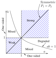
Figure 1: Classes of the two-user ICs.

Among all classes shown in Figure 1, the capacity region of the strong Gaussian IC is fully characterized [3, 2]. In this case, the capacity region can be stated as the collection of all rate pairs $(R_{1},R_{2})$ satisfying

$$\begin{array}[]{rcl}R_{1}&\leq&\gamma{(P_{1})},\\ R_{2}&\leq&\gamma(P_{2}),\\ R_{1}+R_{2}&\leq&\min\left\{\gamma(P_{1}+aP_{2}),\gamma(bP_{1}+P_{2})\right\}.\end{array}$$

II-B Support Functions

Throughout this paper, we use the following facts from convex analysis. There is a one to one correspondence between any closed convex set and its support function [17]. The support function of any set $D\in\Re^{m}$ is a function $\sigma_{D}:\Re^{m}\rightarrow\Re$ defined as

$$\sigma_{D}(\mathbf{c})=\sup\{\mathbf{c}^{t}\mathbf{R}|\mathbf{R}\in D\}.$$ (5)

Clearly, if the set $D$ is compact, then the sup is attained and can be replaced by max. In this case, the solutions of (5) correspond to the boundary points of $D$ [17]. The following relation is the dual of (5) and holds when $D$ is closed and convex

$$D=\{\mathbf{R}|\mathbf{c}^{t}\mathbf{R}\leq\sigma_{D}(\mathbf{c}),\forall~{}\mathbf{c}\}.$$ (6)

For any two closed convex sets $D$ and $D^{\prime}$, $D\subseteq D^{\prime}$, if and only if $\sigma_{D}\leq\sigma_{D^{\prime}}$.

II-C Han-Kobayashi Achievable Region

The best inner bound for the two-user Gaussian IC is the full HK achievable region denoted by $\mathscr{C}_{HK}$ [8]. Despite having a single letter formula, $\mathscr{C}_{HK}$ is not fully characterized yet. In fact, finding the optimum distributions achieving boundary points of $\mathscr{C}_{HK}$ is still an open problem. We define $\mathscr{G}$ as a subset of $\mathscr{C}_{HK}$ where Gaussian distributions are used for codebook generation. Using a shorter description of $\mathscr{C}_{HK}$ obtained in [9], $\mathscr{G}$ can be described as follows.

Let us first define $\mathscr{G}_{0}$ as the collection of all rate pairs $(R_{1},R_{2})\in\Re_{+}^{2}$ satisfying

$$R_{1} \leq\psi_{1}=\gamma\left(\frac{P_{1}}{1+a\beta P_{2}}\right),$$ (7)

$$R_{2} \leq\psi_{2}=\gamma\left(\frac{P_{2}}{1+b\alpha P_{1}}\right),$$ (8)

$$R_{1}+R_{2} \leq\psi_{3}=\min\left\{\psi_{31},\psi_{32},\psi_{33}\right\},$$ (9)

$$2R_{1}+R_{2} \leq\psi_{4}=\gamma\left(\frac{P_{1}+a(1-\beta)P_{2}}{1+a\beta P_{2}}\right)+\gamma\left(\frac{\alpha P_{1}}{1+a\beta P_{2}}\right)+\gamma\left(\frac{\beta P_{2}+b(1-\alpha)P_{1}}{1+b\alpha P_{1}}\right),$$ (10)

$$R_{1}+2R_{2} \leq\psi_{5}=\gamma\left(\frac{\beta P_{2}}{1+b\alpha P_{1}}\right)+\gamma\left(\frac{P_{2}+b(1-\alpha)P_{1}}{1+b\alpha P_{1}}\right)+\gamma\left(\frac{\alpha P_{1}+a(1-\beta)P_{2}}{1+a\beta P_{2}}\right),$$ (11)

for fixed $\alpha\in[0,1]$ and $\beta\in[0,1]$. $\psi_{3}$ is the minimum of $\psi_{31}$, $\psi_{32}$, and $\psi_{33}$ defined as

$$\psi_{31} =\gamma\left(\frac{P_{1}+a(1-\beta)P_{2}}{1+a\beta P_{2}}\right)+\gamma\left(\frac{\beta P_{2}}{1+b\alpha P_{1}}\right),$$ (12)

$$\psi_{32} =\gamma\left(\frac{\alpha P_{1}}{1+a\beta P_{2}}\right)+\gamma\left(\frac{P_{2}+b(1-\alpha)P_{1}}{1+b\alpha P_{1}}\right),$$ (13)

$$\psi_{33} =\gamma\left(\frac{\alpha P_{1}+a(1-\beta)P_{2}}{1+a\beta P_{2}}\right)+\gamma\left(\frac{\beta P_{2}+b(1-\alpha)P_{1}}{1+b\alpha P_{1}}\right).$$ (14)

$\mathscr{G}_{0}$ is a polytope and a function of four variables $P_{1}$, $P_{2}$, $\alpha$, and $\beta$. To emphasize this relation, we may write $\mathscr{G}_{0}(P_{1},P_{2},\alpha,\beta)$ as needed. It is convenient to represent $\mathscr{G}_{0}$ in a matrix form as $\mathscr{G}_{0}=\left\{\mathbf{R}|A\mathbf{R}\leq\Psi(P_{1},P_{2},\alpha,\beta)\right\}$ where $\mathbf{R}=(R_{1},R_{2})^{t}$, $\Psi=(\psi_{1},\psi_{2},\psi_{3},\psi_{4},\psi_{5})^{t}$, and

$$A=\left(\begin{array}[]{ccccc}1&0&1&2&1\\ 0&1&1&1&2\end{array}\right)^{t}.$$

Equivalently, $\mathscr{G}_{0}$ can be represented as the convex hull of its extreme points, i.e., $\mathscr{G}_{0}(P_{1},P_{2},\alpha,\beta)=\text{conv}~{}\{r_{1},r_{2},\ldots,r_{K}\}$, where it is assumed that $\mathscr{G}_{0}$ has $K$ extreme points. It is easy to show that $K\leq 7$.

Now, $\mathscr{G}$ can be defined as a region obtained from enlarging $\mathscr{G}_{0}$ by making use of the time-sharing parameter, i.e., $\mathscr{G}$ is the collection of all rate pairs $\mathbf{R}=(R_{1},R_{2})^{t}$ satisfying

$$A\mathbf{R} \leq\sum_{i=1}^{q}\lambda_{i}\Psi(P_{1i},P_{2i},\alpha_{i},\beta_{i}),$$ (15)

where $q\in\mathbb{N}$ and

$$\sum_{i=1}^{q}\lambda_{i}P_{1i} \leq P_{1},$$ (16)

$$\sum_{i=1}^{q}\lambda_{i}P_{2i} \leq P_{2},$$ (17)

$$\sum_{i=1}^{q}\lambda_{i} =1,$$ (18)

$$\lambda_{i}\geq 0,~{}(\alpha_{i},\beta_{i}) \in[0,1]^{2};~{}\forall i\in\{1,\ldots,q\}.$$ (19)

It is easy to show that $\mathscr{G}$ is a closed, bounded and convex region. In fact, the capacity region $\mathscr{C}$ which contains $\mathscr{G}$ is inside the rectangle defined by inequalities $R_{1}\leq\gamma(P_{1})$ and $R_{2}\leq\gamma(P_{2})$. Moreover, $(0,0)$, $(\gamma(P_{1}),0)$, and $(0,\gamma(P_{2}))$ are extreme points of both $\mathscr{C}$ and $\mathscr{G}$. Hence, to characterize $\mathscr{G}$, we need to obtain all extreme points of $\mathscr{G}$ that are in the interior of the first quadrant (the same argument holds for $\mathscr{C}$). In other words, we need to obtain $\sigma_{\mathscr{G}}(c_{1},c_{2})$, the support function of $\mathscr{G}$, either when $1\leq c_{1}$ and $c_{2}=1$ or when $c_{1}=1$ and $1\leq c_{2}$.

We also define $\mathscr{G}_{1}$ and $\mathscr{G}_{2}$ obtained by enlarging $\mathscr{G}_{0}$ in two different manners. $\mathscr{G}_{1}$ is defined as

$$\mathscr{G}_{1}(P_{1},P_{2})=\bigcup_{(\alpha,\beta)\in[0,1]^{2}}\mathscr{G}_{0}(P_{1},P_{2},\alpha,\beta).$$ (20)

$\mathscr{G}_{1}$ is not necessarily a convex region. Hence, it can be further enlarged by the convex hull operation. $\mathscr{G}_{2}$ is defined as the collection of all rate pairs $\mathbf{R}=(R_{1},R_{2})^{t}$ satisfying

$$\mathbf{R}=\sum_{i=1}^{q^{\prime}}\lambda_{i}\mathbf{R}_{i}$$ (21)

where $q^{\prime}\in\mathbb{N}$ and

$$A\mathbf{R}_{i} \leq\Psi(P_{1i},P_{2i},\alpha_{i},\beta_{i}),$$ (22)

$$\sum_{i=1}^{q^{\prime}}\lambda_{i}P_{1i} \leq P_{1},$$ (23)

$$\sum_{i=1}^{q^{\prime}}\lambda_{i}P_{2i} \leq P_{2},$$ (24)

$$\sum_{i=1}^{q^{\prime}}\lambda_{i} =1,$$ (25)

$$\lambda_{i}\geq 0,~{}(\alpha_{i},\beta_{i}) \in[0,1]^{2};~{}\forall i\in\{1,\ldots,q^{\prime}\}.$$ (26)

It is easy to show that $\mathscr{G}_{2}$ is a closed, bounded and convex region. In fact, $\mathscr{G}_{2}$ is obtained by using the simple method of TD/FD. To see this, let us divide the available frequency band into $q^{\prime}$ sub-bands where $\lambda_{i}$ represents the length of the $i$’th band and $\sum_{i=1}^{q^{\prime}}\lambda_{i}=1$. User 1 and 2 allocate $P_{1i}$ and $P_{2i}$ in the $i$’th sub-band, respectively. Therefore, all rate pairs in $\mathscr{G}_{0}(P_{1i},P_{2i},\alpha_{i},\beta_{i})$ are achievable in the $i$’th sub-band for fixed $(\alpha_{i},\beta_{i})\in[0,1]^{2}$. Hence, all rate pairs in $\sum_{i=1}^{q^{\prime}}\lambda_{i}\mathscr{G}_{0}(P_{1i},P_{2i},\alpha_{i},\beta_{i})$ are achievable provided that $\sum_{i=1}^{q^{\prime}}\lambda_{i}P_{1i}\leq P_{1}$ and $\sum_{i=1}^{q^{\prime}}\lambda_{i}P_{2i}\leq P_{2}$.

Clearly, the chain of inclusions $\mathscr{G}_{0}\subseteq\mathscr{G}_{1}\subseteq\mathscr{G}_{2}\subseteq\mathscr{G}\subseteq\mathscr{C}_{HK}\subseteq\mathscr{C}$ always holds.

II-D Concavification Versus Time-Sharing

In this subsection, we follow two objectives. First, we aim at providing some necessary conditions such that $\mathscr{G}_{2}=\mathscr{G}$. Second, we bound $q$ and $q^{\prime}$ which are parameters involved in the descriptions of $\mathscr{G}$ and $\mathscr{G}_{2}$, respectively. However, we derive the required conditions for the more general case where there are $M$ users in the system. To this end, assume an achievable scheme for an $M$-user channel with the power constraint $\mathbf{P}=[P_{1},P_{2},\ldots,P_{M}]$ is given. The corresponding achievable region can be represented as

$$D_{0}(\mathbf{P},\Theta)=\left\{\mathbf{R}|A\mathbf{R}\leq\Psi(\mathbf{P},\Theta)\right\},$$ (27)

where $A$ is a $K\times M$ matrix and $\Theta\in[0,1]^{M}$. $D_{0}$ is a polyhedron in general, but for the purpose of this paper, it suffices to assume that it is a polytope. Since $D_{0}$ is a convex region, the convex hull operation does not lead to a new enlarged region. However, if the extreme points of the region are not a concave function of $\mathbf{P}$, it is possible to enlarge $D_{0}$ by using two different methods which are explained next. The first method is based on using the time sharing parameter. Let us denote the corresponding region as $D$ which can be written as

$$D=\left\{\mathbf{R}|A\mathbf{R}\leq\sum_{i=1}^{q}\lambda_{i}\Psi(\mathbf{P}_{i},\Theta_{i}),\sum_{i=1}^{q}\lambda_{i}\mathbf{P}_{i}\leq\mathbf{P},\sum_{i=1}^{q}\lambda_{i}=1,\lambda_{i}\geq 0,\Theta_{i}\in[0,1]^{M}~{}\forall i\right\},$$ (28)

where $q\in\mathbb{N}$.

In the second method, we use TD/FD to enlarge the achievable rate region. This results in an achievable region $D_{2}$ represented as

$$D_{2}=\left\{\mathbf{R}=\sum_{i=1}^{q^{\prime}}\lambda_{i}\mathbf{R}_{i}|A\mathbf{R_{i}}\leq\Psi(\mathbf{P}_{i},\Theta_{i}),\sum_{i=1}^{q^{\prime}}\lambda_{i}\mathbf{P}_{i}\leq\mathbf{P},\sum_{i=1}^{q^{\prime}}\lambda_{i}=1,\lambda_{i}\geq 0,\Theta_{i}\in[0,1]^{M}~{}\forall i\right\},$$ (29)

where $q^{\prime}\in\mathbb{N}$. We refer to this method as concavification. It can be readily shown that $D$ and $D_{2}$ are closed and convex, and $D_{2}\subseteq D$. We are interested in situations where the inverse inclusion holds.

The support function of $D_{0}$ is a function of $\mathbf{P}$, $\Theta$, and $\mathbf{c}$. Hence, we have

$$\sigma_{D_{0}}(\mathbf{c},\mathbf{P},\Theta)=\max\{\mathbf{c}^{t}\mathbf{R}|A\mathbf{R}\leq\Psi(\mathbf{P},\Theta)\}.$$ (30)

For fixed $\mathbf{P}$ and $\Theta$, (30) is a linear program. Using strong duality of linear programming, we obtain

$$\sigma_{D_{0}}(\mathbf{c},\mathbf{P},\Theta)=\min\{\mathbf{y}^{t}\Psi(\mathbf{P},\Theta)|A^{t}\mathbf{y}=\mathbf{c},\mathbf{y}\geq 0\}.$$ (31)

In general, $\hat{\mathbf{y}}$, the minimizer of (31), is a function of $\mathbf{P}$, $\Theta$, and $\mathbf{c}$. We say $D_{0}$ possesses the unique minimizer property if $\hat{\mathbf{y}}$ merely depends on $\mathbf{c}$, for all $\mathbf{c}$. In this case, we have

$$\sigma_{D_{0}}(\mathbf{c},\mathbf{P},\Theta)=\hat{\mathbf{y}}^{t}(\mathbf{c})\Psi(\mathbf{P},\Theta),$$ (32)

where $A^{t}\hat{\mathbf{y}}=\mathbf{c}$. This condition means that for any $\mathbf{c}$ the extreme point of $D_{0}$ maximizing the objective $\mathbf{c}^{t}\mathbf{R}$ is an extreme point obtained by intersecting a set of specific hyperplanes. A necessary condition for $D_{0}$ to possess the unique minimizer property is that each inequality in describing $D_{0}$ is either redundant or active for all $\mathbf{P}$ and $\Theta$.

Theorem 1

If $D_{0}$ possesses the unique minimizer property, then $D=D_{2}$.

Proof:

Since $D_{2}\subseteq D$ always holds, we need to show $D\subseteq D_{2}$ which can be equivalently verified by showing $\sigma_{D}\leq\sigma_{D_{2}}$. The support function of $D$ can be written as

$$\sigma_{D}(\mathbf{c},\mathbf{P})=\max\left\{\mathbf{c}^{t}\mathbf{R}|\mathbf{R}\in D\right\}.$$ (33)

By fixing $\mathbf{P}$, $\mathbf{P}_{i}$’s, $\Theta_{i}$’s, and $\lambda_{i}$’s, the above maximization becomes a linear program. Hence, relying on weak duality of linear programming, we obtain

$$\sigma_{D}(\mathbf{c},\mathbf{P})\leq\min_{A^{t}\mathbf{y}=\mathbf{c},\mathbf{y}\geq 0}\mathbf{y}^{t}\sum_{i=1}^{q}\lambda_{i}\Psi(\mathbf{P}_{i},\Theta_{i}).$$ (34)

Clearly, $\hat{\mathbf{y}}(\mathbf{c})$, the solution of (31), is a feasible point for (34) and we have

$$\sigma_{D}(\mathbf{c},\mathbf{P})\leq\hat{\mathbf{y}}^{t}(\mathbf{c})\sum_{i=1}^{q}\lambda_{i}\Psi(\mathbf{P}_{i},\Theta_{i}).$$ (35)

Using (32), we obtain

$$\sigma_{D}(\mathbf{c},\mathbf{P})\leq\sum_{i=1}^{q}\lambda_{i}\sigma_{D_{0}}(\mathbf{c},\mathbf{P}_{i},\Theta_{i}).$$ (36)

Let us assume $\hat{\mathbf{R}}_{i}$ is the maximizer of (30). In this case, we have

$$\sigma_{D}(\mathbf{c},\mathbf{P})\leq\sum_{i=1}^{q}\lambda_{i}\mathbf{c}^{t}\mathbf{\hat{R}}_{i}.$$ (37)

Hence, we have

$$\sigma_{D}(\mathbf{c},\mathbf{P})\leq\mathbf{c}^{t}\sum_{i=1}^{q}\lambda_{i}\mathbf{\hat{R}}_{i}.$$ (38)

By definition, $\sum_{i=1}^{q}\lambda_{i}\mathbf{\hat{R}}_{i}$ is a point in $D_{2}$. Therefore, we conclude

$$\sigma_{D}(\mathbf{c},\mathbf{P})\leq\sigma_{D_{2}}(\mathbf{c},\mathbf{P}).$$ (39)

This completes the proof. ∎

Corollary 1 (Han [18])

If $D_{0}$ is a polymatroid, then $D$=$D_{2}$.

Proof:

It is easy to show that $D_{0}$ possesses the unique minimizer property. In fact, for given $\mathbf{c}$, $\hat{\mathbf{y}}$ can be obtained in a greedy fashion independent of $\mathbf{P}$ and $\Theta$. ∎

In what follows, we upper bound $q$ and $q^{\prime}$.

Theorem 2

The cardinality of the time sharing parameter $q$ in (28) is less than $M+K+1$, where $M$ and $K$ are the dimensions of $\mathbf{P}$ and $\Psi(\mathbf{P})$, respectively. Moreover, if $\Psi(\mathbf{P})$ is a continuous function of $\mathbf{P}$, then $q\leq M+K$.

Proof:

Let us define $E$ as

$$E=\left\{\sum_{i=1}^{q}\lambda_{i}\Psi(\mathbf{P}_{i},\Theta_{i})|\sum_{i=1}^{q}\lambda_{i}\mathbf{P}_{i}\leq\mathbf{P},\sum_{i=1}^{q}\lambda_{i}=1,\lambda_{i}\geq 0,\Theta_{i}\in[0,1]^{M}~{}\forall i\right\}.$$ (40)

In fact, $E$ is the collection of all possible bounds for $D$. To prove $q\leq M+K+1$, we define another region $E_{1}$ as

$$E_{1}=\{(\mathbf{P}^{\prime},\mathbf{S}^{\prime})|0\leq\mathbf{P}^{\prime},\mathbf{S}^{\prime}=\Psi(\mathbf{P}^{\prime},\Theta^{\prime}),\Theta^{\prime}\in[0,1]^{M}\}.$$ (41)

From the direct consequence of the Caratheodory’s theorem [19], the convex hull of $E_{1}$ denoted by $\text{conv}~{}E_{1}$ can be obtained by convex combinations of no more than $M+K+1$ points in $E_{1}$. Moreover, if $\Psi(\mathbf{P}^{\prime},\Theta^{\prime})$ is continuous, then $M+K$ points are sufficient due to the extension of the Caratheodory’s theorem [19]. Now, we define the region $\hat{E}$ as

$$\hat{E}=\{\mathbf{S}^{\prime}|(\mathbf{P}^{\prime},\mathbf{S}^{\prime})\in\text{conv}~{}E_{1},\mathbf{P}^{\prime}\leq\mathbf{P}\}.$$ (42)

Clearly, $\hat{E}\subseteq E$. To show the other inclusion, let us consider a point in $E$, say $S=\sum_{i=1}^{q}\lambda_{i}\Psi(\mathbf{P}_{i},\Theta_{i})$. Since $(\mathbf{P}_{i},\Psi(\mathbf{P}_{i},\Theta_{i}))$ is a point in $E_{1}$, $\sum_{i=1}^{q}\lambda_{i}(\mathbf{P}_{i},\Psi(\mathbf{P}_{i},\Theta_{i}))$ belongs to $\text{conv}~{}E_{1}$. Having $\sum_{i=1}^{q}\lambda_{i}\mathbf{P}_{i}\leq\mathbf{P}$, we conclude $\sum_{i=1}^{q}\lambda_{i}\Psi(\mathbf{P}_{i},\Theta)\in\hat{E}$. Hence, $E\subseteq\hat{E}$. This completes the proof. ∎

Corollary 2 (Etkin, Parakh, and Tse [20])

For the $M$-user Gaussian IC where users use Gaussian codebooks for data transmission and treat the interference as noise, the cardinality of the time sharing parameter is less than $2M$.

Proof:

In this case, $D_{0}=\left\{\mathbf{R}|\mathbf{R}\leq\Psi(\mathbf{P})\right\}$ where both $\mathbf{P}$ and $\Psi(\mathbf{P})$ have dimension $M$ and $\Psi(\mathbf{P})$ is a continuous function of $\mathbf{P}$. Applying Theorem 2 yields the desired result. ∎

In the following theorem, we obtain an upper bound on $q^{\prime}$.

Theorem 3

To characterize boundary points of $D_{2}$, it suffices to set $q^{\prime}\leq M+1$.

Proof:

Let us assume $\hat{\mathbf{R}}$ is a boundary point of $D_{2}$. Hence, there exists $\mathbf{c}$ such that

$$\sigma_{D_{2}}(\mathbf{c},\mathbf{P})=\max_{\mathbf{R}\in D_{2}}\mathbf{c}^{t}\mathbf{R}=\mathbf{c}^{t}\hat{\mathbf{R}},$$ (43)

where $\hat{\mathbf{R}}=\sum_{i=1}^{q^{\prime}}\hat{\lambda}_{i}\hat{\mathbf{R}}_{i}$ and the optimum is achieved for the set of parameters $\hat{\Theta}_{i}$, $\hat{\lambda}_{i}$, and $\hat{\mathbf{P}}_{i}$. The optimization problem in (43) can be written as

$$\sigma_{D_{2}}(\mathbf{c},\mathbf{P})= \max~{}~{}~{}\sum_{i=1}^{q^{\prime}}\lambda_{i}g(\mathbf{c},\mathbf{P}_{i})$$

$$\text{subject to:}~{}\sum_{i=1}^{q^{\prime}}\lambda_{i}=1,~{}\sum_{i=1}^{q^{\prime}}\lambda_{i}\mathbf{P}_{i}\leq\mathbf{P},$$

$$~{}~{}~{}~{}~{}~{}~{}~{}~{}~{}~{}~{}~{}~{}0\leq\lambda_{i},0\leq\mathbf{P}_{i},~{}\forall i\in\{1,2,\ldots,q^{\prime}\},$$

where $g(\mathbf{c},\mathbf{P})$ is defined as

$$g(\mathbf{c},\mathbf{P})= \max\mathbf{c}^{t}\mathbf{R}$$

$$\text{subject to:}~{}A\mathbf{R}\leq\Psi(\mathbf{P},\Theta),~{}0\leq\Theta\leq 1,$$

In fact, $\sigma_{D_{2}}(\mathbf{c},\mathbf{P})$ in (II-D) can be viewed as the result of the concavification of $g(\mathbf{c},\mathbf{P})$ [19]. Hence, using Theorem 2.16 in [19], we conclude that $q^{\prime}\leq M+1$. ∎

Remarkable point about Theorem 3 is that the upper bound on $q^{\prime}$ is independent of the number of inequalities involved in the description of the achievable rate region.

Corollary 3

For the $M$-user Gaussian IC where users use Gaussian codebooks and treat the interference as noise, we have $D_{2}=D$ and $q=q^{\prime}=M+1$.

II-E Extremal Inequality

In [14], the following optimization problem is studied:

$$W=\max_{Q_{\mathbf{X}}\leq S}h(\mathbf{X}+\mathbf{Z}_{1})-\mu h(\mathbf{X}+\mathbf{Z}_{2}),$$ (46)

where $\mathbf{Z}_{1}$ and $\mathbf{Z}_{2}$ are $n$-dimensional Gaussian random vectors with the strictly positive definite covariance matrices $Q_{\mathbf{Z}_{1}}$ and $Q_{\mathbf{Z}_{2}}$, respectively. The optimization is over all random vectors $\mathbf{X}$ independent of $\mathbf{Z}_{1}$ and $\mathbf{Z}_{2}$. $\mathbf{X}$ is also subject to the covariance matrix constraint $Q_{\mathbf{X}}\leq S$, where $S$ is a positive definite matrix. In [14], it is shown that for all $\mu\geq 1$, this optimization problem has a Gaussian optimal solution for all positive definite matrices $Q_{\mathbf{Z}_{1}}$ and $Q_{\mathbf{Z}_{2}}$. However, for $0\leq\mu<1$ this optimization problem has a Gaussian optimal solution provided $Q_{\mathbf{Z}_{1}}\leq Q_{\mathbf{Z}_{2}}$, i.e., $Q_{\mathbf{Z}_{2}}-Q_{\mathbf{Z}_{1}}$ is a positive semi-definite matrix. It is worth noting that for $\mu=1$ this problem when $Q_{\mathbf{Z}_{1}}\leq Q_{\mathbf{Z}_{2}}$ is studied under the name of the worse additive noise [21, 22].

In this paper, we consider a special case of (46) where $\mathbf{Z}_{1}$ and $\mathbf{Z}_{2}$ have the covariance matrices $N_{1}I$ and $N_{2}I$, respectively, and the trace constraint is considered, i.e.,

$$W=\max_{tr\{Q_{\mathbf{X}}\}\leq nP}h(\mathbf{X}+\mathbf{Z}_{1})-\mu h(\mathbf{X}+\mathbf{Z}_{2}).$$ (47)

In the following lemma, we provide the optimal solution for the above optimization problem when $N_{1}\leq N_{2}$.

Lemma 1

If $N_{1}\leq N_{2}$, the optimal solution of (47) is iid Gaussian for all $0\leq\mu$ and we have

1. For $0\leq\mu\leq\frac{N_{2}+P}{N_{1}+P}$, the optimum covariance matrix is $PI$ and the optimum solution is

   $$W=\frac{n}{2}\log\left[(2\pi e)(P+N_{1})\right]-\frac{\mu n}{2}\log\left[(2\pi e)(P+N_{2})\right].$$ (48)

2. For $\frac{N_{2}+P}{N_{1}+P}<\mu\leq\frac{N_{2}}{N_{1}}$, the optimum covariance matrix is $\frac{N_{2}-\mu N_{1}}{\mu-1}I$ and the optimum solution is

   $$W=\frac{n}{2}\log\left[(2\pi e)\frac{N_{2}-N_{1}}{\mu-1}\right]-\frac{\mu n}{2}\log\left[\frac{\mu(2\pi e)(N_{2}-N_{1})}{\mu-1}\right].$$ (49)

3. For $\frac{N_{2}}{N_{1}}<\mu$, the optimum covariance matrix is $0$ and the optimum solution is

   $$W=\frac{n}{2}\log(2\pi eN_{1})-\frac{\mu n}{2}\log(2\pi eN_{2}).$$ (50)

Proof:

From the general result for (46), we know that the optimum input distribution is Gaussian. Hence, we need to solve the following maximization problem:

$$W= \max\frac{1}{2}\log\left((2\pi e)^{n}|Q_{\mathbf{X}}+N_{1}I|\right)-\frac{\mu}{2}\log\left((2\pi e)^{n}|Q_{\mathbf{X}}+N_{2}I|\right)$$

$$\text{subject to:}~{}0\leq Q_{\mathbf{X}},~{}tr\{Q_{\mathbf{X}}\}\leq nP.$$

Since $Q_{\mathbf{X}}$ is a positive semi-definite matrix, it can be decomposed as $Q_{\mathbf{X}}=U\Lambda U^{t}$, where $\Lambda$ is a diagonal matrix with nonnegative entries and $U$ is a unitary matrix, i.e., $UU^{t}=I$. Substituting $Q_{\mathbf{X}}=U\Lambda U^{t}$ in (II-E) and using the identities $tr\{AB\}=tr\{BA\}$ and $|AB+I|=|BA+I|$, we obtain

$$W= \max\frac{1}{2}\log\left((2\pi e)^{n}|\Lambda+N_{1}I|\right)-\frac{\mu}{2}\log\left((2\pi e)^{n}|\Lambda+N_{2}I|\right)$$

$$\text{subject to:}~{}0\leq\Lambda,~{}tr\{\Lambda\}\leq nP.$$

This optimization problem can be simplified as

$$W= \max\frac{n}{2}\sum_{i=1}^{n}\left[\log(2\pi e)(\lambda_{i}+N_{1})-\mu\log(2\pi e)(\lambda_{i}+N_{2})\right]$$

$$\text{subject to:}~{}0\leq\lambda_{i}~{}\forall i,~{}\sum_{i=1}^{n}\lambda_{i}\leq nP.$$

By introducing Lagrange multipliers $\psi$ and $\Phi=\{\phi_{1},\phi_{2},\ldots,\phi_{n}\}$, we obtain

$$L(\Lambda,\psi,\Phi)=\max\frac{n}{2}\sum_{i=1}^{n}\left[\log(2\pi e)(\lambda_{i}+N_{1})-\mu\log(2\pi e)(\lambda_{i}+N_{2})\right]+\psi\left(nP-\sum_{i=1}^{n}\lambda_{i}\right)+\sum_{i=1}^{n}\phi_{i}\lambda_{i}.$$ (54)

The first order KKT necessary conditions for the optimum solution of (54) can be written as

$$\frac{1}{\lambda_{i}+N_{1}}-\frac{\mu}{\lambda_{i}+N_{2}}-\psi+\phi_{i}= 0,~{}\forall i\in\{1,2,\ldots,n\},$$ (55)

$$\psi\left(nP-\sum_{i=1}^{n}\lambda_{i}\right)= 0,$$ (56)

$$\phi_{i}\lambda_{i}= 0,~{}\forall i\in\{1,2,\ldots,n\}.$$ (57)

It is easy to show that when $N_{1}\leq N_{2}$, $\lambda=\lambda_{1}=\ldots=\lambda_{n}$ and the only solution for $\lambda$ is

$$\lambda=\left\{\begin{array}[]{llrl}P,&~{}\text{if}{}&0&\leq\mu\leq\frac{N_{2}+P}{N_{1}+P}\\ \frac{N_{2}-\mu N_{1}}{\mu-1},&~{}\text{if}{}&\frac{N_{2}+P}{N_{1}+P}&<\mu\leq\frac{N_{2}}{N_{1}}\\ 0,&~{}\text{if}{}&\frac{N_{2}}{N_{1}}&<\mu\end{array}\right.$$ (58)

Substituting $\lambda$ into the objective function gives the desired result. ∎

In Figure 2, the optimum variance as a function of $\mu$ is plotted. This figure shows that for any value of $\mu\leq\frac{P+N_{2}}{P+N_{1}}$, we need to use the maximum power to optimize the objective function, whereas for $\mu>\frac{P+N_{2}}{P+N_{1}}$, we use less power than what is permissible.

Figure 2: Optimum variance versus $\mu$.

Lemma 2

If $N_{1}>N_{2}$, the optimal solution of (47) is iid Gaussian for all $1\leq\mu$. In this case, the optimum variance is $0$ and the optimum $W$ is

$$W=\frac{n}{2}\log(2\pi eN_{1})-\frac{\mu n}{2}\log(2\pi eN_{2}).$$ (59)

Proof:

The proof is similar to that of Lemma 1 and we omit it here. ∎

Corollary 4

For $\mu=1$, the optimal solution of (47) is iid Gaussian and the optimum $W$ is

$$W=\left\{\begin{array}[]{ll}\frac{n}{2}\log\left(\frac{P+N_{1}}{P+N_{2}}\right),&\text{if}~{}N_{1}\leq N_{2}\\ \frac{n}{2}\log\left(\frac{N_{1}}{N_{2}}\right),&\text{if}~{}N_{1}>N_{2}.\end{array}\right.$$ (60)

We frequently apply the following optimization problem in the rest of the paper:

$$f_{h}(P,N_{1},N_{2},a,\mu)=\max_{tr\{Q_{\mathbf{X}}\}\leq nP}h(\mathbf{X}+\mathbf{Z}_{1})-\mu h(\sqrt{a}\mathbf{X}+\mathbf{Z}_{2}),$$ (61)

where $N_{1}\leq N_{2}/a$. Using the identity $h(A\mathbf{X})=\log(|A|)+h(\mathbf{X})$, (61) can be written as

$$f_{h}(P,N_{1},N_{2},a,\mu)=\frac{n}{2}\log a+\max_{tr\{Q_{\mathbf{X}}\}\leq nP}h(\mathbf{X}+\mathbf{Z}_{1})-\mu h(\mathbf{X}+\frac{\mathbf{Z}_{2}}{\sqrt{a}}).$$ (62)

Now, Lemma 1 can be applied to obtain

$$f_{h}(P,N_{1},N_{2},a,\mu)=\left\{\begin{array}[]{ll}\frac{1}{2}\log\left[(2\pi e)(P+N_{1})\right]-\frac{\mu}{2}\log\left[(2\pi e)(aP+N_{2})\right]&~{}\text{if}~{}0\leq\mu\leq\frac{P+N_{2}/a}{P+N_{1}}\\ \frac{1}{2}\log\left[(2\pi e)\frac{N_{2}/a-N_{1}}{\mu-1}\right]-\frac{\mu}{2}\log\left[\frac{a\mu(2\pi e)(N_{2}/a-N_{1})}{\mu-1}\right]&~{}\text{if}~{}\frac{P+N_{2}/a}{P+N_{1}}<\mu\leq\frac{N_{2}}{aN_{1}}\\ \frac{1}{2}\log(2\pi eN_{1})-\frac{\mu}{2}\log(2\pi eN_{2})&~{}\text{if}~{}\frac{N_{2}}{aN_{1}}<\mu\end{array}\right.$$ (63)

III Admissible Channels

In this section, we aim at building ICs whose capacity regions contain the capacity region of the two-user Gaussian IC, i.e., $\mathscr{C}$. Since we ultimately use these to outer bound $\mathscr{C}$, these ICs need to have a tractable expression (or a tractable outer bound) for their capacity regions.

Let us consider an IC with the same input letters as that of $\mathscr{C}$ and the output letters $\tilde{y}_{1}$ and $\tilde{y}_{2}$ for Users 1 and 2, respectively. The capacity region of this channel, say $\mathscr{C}^{\prime}$, contains $\mathscr{C}$ if

$$I(x_{1}^{n};y_{1}^{n})\leq I(x_{1}^{n};\tilde{y}_{1}^{n}),$$ (64)

$$I(x_{2}^{n};y_{2}^{n})\leq I(x_{2}^{n};\tilde{y}_{2}^{n}),$$ (65)

for all $p(x_{1}^{n})p(x_{2}^{n})$ and for all $n\in\mathbb{N}$.

One way to satisfy (64) and (65) is to provide some extra information to either one or to both receivers. This technique is known as Genie aided outer bounding. In [12], Kramer has used such a genie to provide some extra information to both receivers such that they can decode both users’ messages. Since the capacity region of this new interference channel is equivalent to that of the Compound Multiple Access Channel whose capacity region is known, reference [12] obtains an outer bound on the capacity region. To obtain a tighter outer bound, reference [12] further uses the fact that if a genie provides the exact information about the interfering signal to one of the receivers, then the new channel becomes the one-sided Gaussian IC. Although the capacity region of the one-sided Gaussian IC is unknown for all ranges of parameters, there exists an outer bound for it due to Sato and Costa [23, 11] that can be applied to the original channel. In [13], Etkin et al. use a different genie that provides some extra information about the intended signal. Even though at first glance their proposed method appears to be far from achieving a tight bound, remarkably they show that the corresponding bound is tighter than the one due to Kramer for certain ranges of parameters.

Next, we introduce the notion of admissible channels to satisfy (64) and (65).

Definition 3 (Admissible Channel)

An IC $\mathscr{C}^{\prime}$ with input letter $x_{i}$ and output letter $\tilde{y}_{i}$ for User $i\in\{1,2\}$ is an admissible channel if there exist two deterministic functions $\hat{y}_{1}^{n}=f_{1}(\tilde{y}_{1}^{n})$ and $\hat{y}_{2}^{n}=f_{2}(\tilde{y}_{2}^{n})$ such that

$$I(x_{1}^{n};y_{1}^{n})\leq I(x_{1}^{n};\hat{y}_{1}^{n}),$$ (66)

$$I(x_{2}^{n};y_{2}^{n})\leq I(x_{2}^{n};\hat{y}_{2}^{n})$$ (67)

hold for all $p(x_{1}^{n})p(x_{2}^{n})$ and for all $n\in\mathbb{N}$. $\mathscr{E}$ denotes the collection of all admissible channels (see Figure 3).

Figure 3: An admissible channel. $f_{1}$ and $f_{2}$ are deterministic functions.

Remark 2

Genie aided channels are among admissible channels. To see this, let us assume a genie provides $s_{1}$ and $s_{2}$ as side information for User 1 and 2, respectively. In this case, $\tilde{y}_{i}=(y_{i},s_{i})$ for $i\in\{1,2\}$. By choosing $f_{i}(y_{i},s_{i})=y_{i}$, we observe that $\hat{y}_{i}=y_{i}$, and hence, (66) and (67) trivially hold.

To obtain the tightest outer bound, we need to find the intersection of the capacity regions of all admissible channels. Nonetheless, it may happen that finding the capacity region of an admissible channel is as hard as that of the original one (in fact, based on the definition, the channel itself is one of its admissible channels). Hence, we need to find classes of admissible channels, say $\mathscr{F}$, which possess two important properties. First, their capacity regions are close to $\mathscr{C}$. Second, either their exact capacity regions are computable or there exist good outer bounds for them. Since $\mathscr{F}\subseteq\mathscr{E}$, we have

$$\mathscr{C}\subseteq\bigcap_{\mathscr{F}}\mathscr{C}^{\prime}.$$ (68)

Recall that there is a one to one correspondence between a closed convex set and its support function. Since $\mathscr{C}$ is closed and convex, there is a one to one correspondence between $\mathscr{C}$ and $\sigma_{\mathscr{C}}$. In fact, boundary points of $\mathscr{C}$ correspond to the solutions of the following optimization problem

$$\sigma_{\mathscr{C}}(c_{1},c_{2})=\max_{(R_{1},R_{2})\in\mathscr{C}}c_{1}R_{1}+c_{2}R_{2}.$$ (69)

Since we are interested in the boundary points excluding the $R_{1}$ and $R_{2}$ axes, it suffices to consider $0\leq c_{1}$ and $0\leq c_{2}$ where $c_{1}+c_{2}=1$.

Since $\mathscr{C}\subseteq\mathscr{C}^{\prime}$, we have

$$\sigma_{\mathscr{C}}(c_{1},c_{2})\leq\sigma_{\mathscr{C}^{\prime}}(c_{1},c_{2}).$$ (70)

Taking the minimum of the right hand side, we obtain

$$\sigma_{\mathscr{C}}(c_{1},c_{2})\leq\min_{\mathscr{C}^{\prime}\in\mathscr{F}}\sigma_{\mathscr{C}^{\prime}}(c_{1},c_{2}),$$ (71)

which can be written as

$$\sigma_{\mathscr{C}}(c_{1},c_{2})\leq\min_{\mathscr{C}^{\prime}\in\mathscr{F}}\max_{(R_{1},R_{2})\in\mathscr{C}^{\prime}}c_{1}R_{1}+c_{2}R_{2}.$$ (72)

For convenience, we use the following two optimization problems

$$\sigma_{\mathscr{C}}(\mu,1)=\max_{(R_{1},R_{2})\in\mathscr{C}}\mu R_{1}+R_{2},$$ (73)

$$\sigma_{\mathscr{C}}(1,\mu)=\max_{(R_{1},R_{2})\in\mathscr{C}}R_{1}+\mu R_{2},$$ (74)

where $1\leq\mu$. It is easy to show that the solutions of (73) and (74) correspond to the boundary points of the capacity region.

In the rest of this section, we introduce classes of admissible channels and obtain upper bounds on $\sigma_{\mathscr{C}^{\prime}}(\mu,1)$ and $\sigma_{\mathscr{C}^{\prime}}(1,\mu)$.

III-A Classes of Admissible Channels

III-A1 Class A1

This class is designed to obtain an upper bound on $\sigma_{\mathscr{C}}(\mu,1)$. Therefore, we need to find a tight upper bound on $\sigma_{\mathscr{C}^{\prime}}(\mu,1)$. A member of this class is a channel in which User 1 has one transmit and one receive antenna whereas User 2 has one transmit antenna and two receive antennas (see Figure 4). The channel model can be written as

$$\begin{array}[]{rl}\tilde{y}_{1}=&x_{1}+\sqrt{a}x_{2}+z_{1},\\ \tilde{y}_{21}=&x_{2}+\sqrt{b^{\prime}}x_{1}+z_{21},\\ \tilde{y}_{22}=&x_{2}+z_{22},\end{array}$$ (75)

where $\tilde{y}_{1}$ is the signal at the first receiver, $\tilde{y}_{21}$ and $\tilde{y}_{22}$ are the signals at the second receiver, $z_{1}$ is additive Gaussian noise with unit variance, $z_{21}$ and $z_{22}$ are additive Gaussian noise with variances $N_{21}$ and $N_{22}$, respectively. Transmitters 1 and 2 are subject to the power constraints of $P_{1}$ and $P_{2}$, respectively.

Figure 4: Class A1 admissible channels.

To investigate admissibility conditions in (66) and (67), we introduce two deterministic functions $f_{1}$ and $f_{2}$ as follows (see Figure 4)

$$f_{1}(\tilde{y}_{1}^{n}) =\tilde{y}_{1}^{n},$$ (76)

$$f_{2}(\tilde{y}_{22}^{n},\tilde{y}_{21}^{n}) =(1-\sqrt{g_{2}})\tilde{y}_{22}^{n}+\sqrt{g_{2}}\tilde{y}_{21}^{n},$$ (77)

where $0\leq g_{2}$. For $g_{2}=0$, the channel can be converted to the one-sided Gaussian IC by letting $N_{21}\rightarrow\infty$ and $N_{22}=1$. Hence, Class A1 contains the one-sided Gaussian IC obtained by removing the link between Transmitter 1 and Receiver 2. Using $f_{1}$ and $f_{2}$, we obtain

$$\hat{y}_{1}^{n}= x_{1}^{n}+\sqrt{a}x_{2}^{n}+z_{1}^{n},$$ (78)

$$\hat{y}_{2}^{n}= \sqrt{b^{\prime}g_{2}}x_{1}^{n}+x_{2}^{n}+(1-\sqrt{g_{2}})z_{22}^{n}+\sqrt{g_{2}}z_{21}^{n}.$$ (79)

Hence, this channel is admissible if the corresponding parameters satisfy

$$\begin{array}[]{rl}b^{\prime}g_{2}&=b,\\ (1-\sqrt{g_{2}})^{2}N_{22}+g_{2}N_{21}&=1.\end{array}$$ (80)

We further add the following constraints to the conditions of the channels in Class A1:

$$\begin{array}[]{rl}b^{\prime}&\leq N_{21},\\ aN_{22}&\leq 1.\end{array}$$ (81)

Although these additional conditions reduce the number of admissible channels within the class, they are needed to get a closed form formula for an upper bound on $\sigma_{\mathscr{C}^{\prime}}(\mu,1)$. In the following lemma, we obtain the required upper bound.

Lemma 3

For the channels modeled by (75) and satisfying (81), we have

$$\sigma_{\mathscr{C}^{\prime}}(\mu,1)\leq \min\frac{\mu_{1}}{2}\log\left[2\pi e(P_{1}+aP_{2}+1)\right]-\frac{\mu_{2}}{2}\log(2\pi e)+\frac{1}{2}\log\left(\frac{N_{21}}{N_{22}}+\frac{b^{\prime}P_{1}}{N_{22}}+\frac{P_{2}}{P_{2}+N_{22}}\right)$$

$$~{}~{}~{}~{}~{}~{}~{}~{}~{}~{}~{}~{}+\mu_{2}f_{h}\left(P_{1},1,N_{21},b^{\prime},\frac{1}{\mu_{2}}\right)+f_{h}(P_{2},N_{22},1,a,\mu_{1})$$

$$\text{subject to:}~{}\mu_{1}+\mu_{2}=\mu,~{}\mu_{1},\mu_{2}\geq 0.$$

Proof:

Let us assume $R_{1}$ and $R_{2}$ are achievable rates for User 1 and 2, respectively. Furthermore, we split $\mu$ into $\mu_{1}\geq 0$ and $\mu_{2}\geq 0$ such that $\mu=\mu_{1}+\mu_{2}$. Using Fano’s inequality, we obtain

$$n(\mu R_{1}+R_{2})\stackrel{{\scriptstyle}}{{\leq}} \mu I(x_{1}^{n};\tilde{y}_{1}^{n})+I(x_{2}^{n};\tilde{y}_{22}^{n},\tilde{y}_{21}^{n})+n\epsilon_{n}$$

$$\stackrel{{\scriptstyle}}{{=}} \mu_{1}I(x_{1}^{n};\tilde{y}_{1}^{n})+\mu_{2}I(x_{1}^{n};\tilde{y}_{1}^{n})+I(x_{2}^{n};\tilde{y}_{22}^{n},\tilde{y}_{21}^{n})+n\epsilon_{n}$$

$$\stackrel{{\scriptstyle(a)}}{{\leq}} \mu_{1}I(x_{1}^{n};\tilde{y}_{1}^{n})+\mu_{2}I(x_{1}^{n};\tilde{y}_{1}^{n}|x_{2}^{n})+I(x_{2}^{n};\tilde{y}_{22}^{n},\tilde{y}_{21}^{n})+n\epsilon_{n}$$

$$\stackrel{{\scriptstyle}}{{=}} \mu_{1}I(x_{1}^{n};\tilde{y}_{1}^{n})+\mu_{2}I(x_{1}^{n};\tilde{y}_{1}^{n}|x_{2}^{n})+I(x_{2}^{n};\tilde{y}_{21}^{n}|\tilde{y}_{22}^{n})+I(x_{2}^{n};\tilde{y}_{22}^{n})+n\epsilon_{n}$$

$$\stackrel{{\scriptstyle}}{{=}} \mu_{1}h(\tilde{y}_{1}^{n})-\mu_{1}h(\tilde{y}_{1}^{n}|x_{1}^{n})+\mu_{2}h(\tilde{y}_{1}^{n}|x_{2}^{n})-\mu_{2}h(\tilde{y}_{1}^{n}|x_{1}^{n},x_{2}^{n})$$

$$+h(\tilde{y}_{21}^{n}|\tilde{y}_{22}^{n})-h(\tilde{y}_{21}^{n}|x_{2}^{n},\tilde{y}_{22}^{n})+h(\tilde{y}_{22}^{n})-h(\tilde{y}_{22}^{n}|x_{2}^{n})+n\epsilon_{n}$$

$$\stackrel{{\scriptstyle}}{{=}} \big{[}\mu_{1}h(\tilde{y}_{1}^{n})-\mu_{2}h(\tilde{y}_{1}^{n}|x_{1}^{n},x_{2}^{n})\big{]}+\big{[}\mu_{2}h(\tilde{y}_{1}^{n}|x_{2}^{n})-h(\tilde{y}_{21}^{n}|x_{2}^{n},\tilde{y}_{22}^{n})\big{]}$$ (83)

$$+\big{[}h(\tilde{y}_{21}^{n}|\tilde{y}_{22}^{n})-h(\tilde{y}_{22}^{n}|x_{2}^{n})\big{]}+\big{[}h(\tilde{y}_{22}^{n})-\mu_{1}h(\tilde{y}_{1}^{n}|x_{1}^{n})\big{]}+n\epsilon_{n},$$

where (a) follows from the fact that $x_{1}^{n}$ and $x_{2}^{n}$ are independent. Now, we separately upper bound the terms within each bracket in (83).

To maximize the terms within the first bracket, we use the fact that Gaussian distribution maximizes the differential entropy subject to a constraint on the covariance matrix. Hence, we have

$$\mu_{1}h(\tilde{y}_{1}^{n})-\mu_{2}h(\tilde{y}_{1}^{n}|x_{1}^{n},x_{2}^{n}) =\mu_{1}h(x_{1}^{n}+\sqrt{a}x_{2}^{n}+z_{1}^{n})-\mu_{2}h(z_{1}^{n})$$ (84)

$$\leq\frac{\mu_{1}n}{2}\log\left[2\pi e(P_{1}+aP_{2}+1)\right]-\frac{\mu_{2}n}{2}\log(2\pi e).$$

Since $b^{\prime}\leq N_{21}$, we can make use of Lemma 1 to upper bound the second bracket. In this case, we have

$$\mu_{2}h(\tilde{y}_{1}^{n}|x_{2}^{n})-h(\tilde{y}_{21}^{n}|x_{2}^{n},\tilde{y}_{22}^{n}) =\mu_{2}\left(h(x_{1}^{n}+z_{1}^{n})-\frac{1}{\mu_{2}}h(\sqrt{b^{\prime}}x_{1}^{n}+z_{21}^{n})\right)$$ (85)

$$\leq\mu_{2}nf_{h}\left(P_{1},1,N_{21},b^{\prime},\frac{1}{\mu_{2}}\right),$$

where $f_{h}$ is defined in (63).

We upper bound the terms within the third bracket as follows [13]:

$$h(\tilde{y}_{21}^{n}|\tilde{y}_{22}^{n})-h(\tilde{y}_{22}^{n}|x_{2}^{n})\stackrel{{\scriptstyle(a)}}{{\leq}} \sum_{i=1}^{n}h(\tilde{y}_{21}[i]|\tilde{y}_{22}[i])-h(z_{22}^{n})$$

$$\stackrel{{\scriptstyle(b)}}{{\leq}} \sum_{i=1}^{n}\frac{1}{2}\log\left[2\pi e\left(N_{21}+b^{\prime}P_{1}[i]+\frac{P_{2}[i]N_{22}}{P_{2}[i]+N_{22}}\right)\right]-\frac{n}{2}\log\left(2\pi eN_{22}\right)$$

$$\stackrel{{\scriptstyle(c)}}{{\leq}} \frac{n}{2}\log\left[2\pi e\left(N_{21}+\frac{1}{n}\sum_{i=1}^{n}b^{\prime}P_{1}[i]+\frac{\frac{1}{n}\sum_{i=1}^{n}P_{2}[i]N_{22}}{\frac{1}{n}\sum_{i=1}^{n}P_{2}[i]+N_{22}}\right)\right]-\frac{n}{2}\log\left(2\pi eN_{22}\right)$$

$$\stackrel{{\scriptstyle}}{{\leq}} \frac{n}{2}\log\left[2\pi e\left(N_{21}+b^{\prime}P_{1}+\frac{P_{2}N_{22}}{P_{2}+N_{22}}\right)\right]-\frac{n}{2}\log\left(2\pi eN_{22}\right)$$

$$\stackrel{{\scriptstyle}}{{\leq}} \frac{n}{2}\log\left(\frac{N_{21}}{N_{22}}+\frac{b^{\prime}P_{1}}{N_{22}}+\frac{P_{2}}{P_{2}+N_{22}}\right),$$ (86)

where (a) follows from the chain rule and the fact that removing independent conditions does not decrease differential entropy, (b) follows from the fact that Gaussian distribution maximizes the conditional entropy for a given covariance matrix, and (c) follows form Jenson’s inequality.

For the last bracket, we again make use of the definition of $f_{h}$. In fact, since $aN_{22}\leq 1$, we have

$$h(\tilde{y}_{22}^{n})-\mu_{1}h(\tilde{y}_{1}^{n}|x_{1}^{n}) =h(x_{2}^{n}+z_{22}^{n})-\mu_{1}h(\sqrt{a}x_{2}^{n}+z_{1}^{n})$$ (87)

$$\leq nf_{h}(P_{2},N_{22},1,a,\mu_{1}).$$

Adding all inequalities, we obtain

$$\mu R_{1}+R_{2}\leq \frac{\mu_{1}}{2}\log\left[2\pi e(P_{1}+aP_{2}+1)\right]-\frac{\mu_{2}}{2}\log(2\pi e)+\frac{1}{2}\log\left(\frac{N_{21}}{N_{22}}+\frac{b^{\prime}P_{1}}{N_{22}}+\frac{P_{2}}{P_{2}+N_{22}}\right)$$ (88)

$$+\mu_{2}f_{h}\left(P_{1},1,N_{21},b^{\prime},\frac{1}{\mu_{2}}\right)+f_{h}(P_{2},N_{22},1,a,\mu_{1}),$$

where the fact that $\epsilon_{n}\rightarrow 0$ as $n\rightarrow\infty$ is used to eliminate $\epsilon_{n}$ form the right hand side of the inequality. Now, by taking the minimum of the right hand side of (88) over all $\mu_{1}$ and $\mu_{2}$, we obtain the desired result. This completes the proof. ∎

III-A2 Class A2

This class is the complement of Class A1 in the sense that we use it to upper bound $\sigma_{\mathscr{C}}(1,\mu)$. A member of this class is a channel in which User 1 is equipped with one transmit and two receive antennas, whereas User 2 is equipped with one antenna at both transmitter and receiver sides (see Figure 5). The channel model can be written as

$$\begin{array}[]{rl}\tilde{y}_{11}=&x_{1}+z_{11},\\ \tilde{y}_{12}=&x_{1}+\sqrt{a^{\prime}}x_{2}+z_{12},\\ \tilde{y}_{2}=&x_{2}+\sqrt{b}x_{1}+z_{2},\end{array}$$ (89)

where $\tilde{y}_{11}$ and $\tilde{y}_{12}$ are the signals at the first receiver, $\tilde{y}_{2}$ is the signal at the second receiver, $z_{2}$ is additive Gaussian noise with unit variance, $z_{11}$ and $z_{12}$ are additive Gaussian noise with variances $N_{11}$ and $N_{12}$, respectively. Transmitter 1 and 2 are subject to the power constraints $P_{1}$ and $P_{2}$, respectively.

Figure 5: Class A2 admissible channels.

For this class, we consider two linear functions $f_{1}$ and $f_{2}$ as follows (see Figure 5):

$$f_{1}(\tilde{y}_{11}^{n},\tilde{y}_{12}^{n}) =(1-\sqrt{g_{1}})\tilde{y}_{11}^{n}+\sqrt{g_{1}}\tilde{y}_{12}^{n},$$ (90)

$$f_{2}(\tilde{y}_{2}^{n}) =\tilde{y}_{2}^{n}.$$ (91)

Similar to Class A1, when $g_{1}=0$, the admissible channels in Class A2 become the one-sided Gaussian IC by letting $N_{12}\rightarrow\infty$ and $N_{11}=1$. Therefore, we have

$$\hat{y}_{1}^{n}= x_{1}^{n}+\sqrt{a^{\prime}g_{1}}x_{2}^{n}+(1-\sqrt{g_{1}})z_{11}^{n}+\sqrt{g_{1}}z_{12}^{n},$$ (92)

$$\hat{y}_{2}^{n}= \sqrt{b}x_{1}^{n}+x_{2}^{n}+z_{2}^{n}.$$ (93)

We conclude that the channel modeled by (89) is admissible if the corresponding parameters satisfy

$$\begin{array}[]{rl}a^{\prime}g_{1}&=a,\\ (1-\sqrt{g_{1}})^{2}N_{11}+g_{1}N_{12}&=1.\end{array}$$ (94)

Similar to Class A1, we further add the following constraints to the conditions of Class A2 channels:

$$\begin{array}[]{rl}a^{\prime}&\leq N_{12},\\ bN_{11}&\leq 1.\end{array}$$ (95)

In the following lemma, we obtain the required upper bound.

Lemma 4

For the channels modeled by (89) and satisfying (95), we have

$$\sigma_{\mathscr{C}^{\prime}}(1,\mu)\leq \min\frac{\mu_{1}}{2}\log\left[2\pi e(bP_{1}+P_{2}+1)\right]-\frac{\mu_{2}}{2}\log(2\pi e)+\frac{1}{2}\log\left(\frac{N_{12}}{N_{11}}+\frac{a^{\prime}P_{2}}{N_{11}}+\frac{P_{1}}{P_{1}+N_{11}}\right)$$

$$~{}~{}~{}~{}~{}~{}~{}~{}~{}~{}~{}~{}+\mu_{2}f_{h}\left(P_{2},1,N_{12},a^{\prime},\frac{1}{\mu_{2}}\right)+f_{h}(P_{1},N_{11},1,b,\mu_{1})$$

$$\text{subject to:}~{}\mu_{1}+\mu_{2}=\mu,~{}\mu_{1},\mu_{2}\geq 0.$$

Proof:

The proof is similar to that of Lemma 3 and we omit it here. ∎

III-A3 Class B

A member of this class is a channel with one transmit antenna and two receive antennas for each user modeled by (see Figure 6)

$$\begin{array}[]{rl}\tilde{y}_{11}=&x_{1}+z_{11},\\ \tilde{y}_{12}=&x_{1}+\sqrt{a^{\prime}}x_{2}+z_{12},\\ \tilde{y}_{21}=&x_{2}+\sqrt{b^{\prime}}x_{1}+z_{21},\\ \tilde{y}_{22}=&x_{2}+z_{22},\end{array}$$ (97)

where $\tilde{y}_{11}$ and $\tilde{y}_{12}$ are the signals at the first receiver, $\tilde{y}_{21}$ and $\tilde{y}_{22}$ are the signals at the second receiver, and $z_{ij}$ is additive Gaussian noise with variance $N_{ij}$ for $i,j\in\{1,2\}$. Transmitter 1 and 2 are subject to the power constraints $P_{1}$ and $P_{2}$, respectively. In fact, this channel is designed to upper bound both $\sigma_{\mathscr{C}}(\mu,1)$ and $\sigma_{\mathscr{C}}(1,\mu)$.

Figure 6: Class B admissible channels.

Next, we investigate admissibility of this channel and the conditions that must be imposed on the underlying parameters. Let us consider two linear deterministic functions $f_{1}$ and $f_{2}$ with parameters $0\leq g_{1}$ and $0\leq g_{2}$, respectively, as follows (see Figure 6)

$$f_{1}(\tilde{y}_{11}^{n},\tilde{y}_{12}^{n}) =(1-\sqrt{g_{1}})\tilde{y}_{11}^{n}+\sqrt{g_{1}}\tilde{y}_{12}^{n},$$ (98)

$$f_{2}(\tilde{y}_{22}^{n},\tilde{y}_{21}^{n}) =(1-\sqrt{g_{2}})\tilde{y}_{22}^{n}+\sqrt{g_{2}}\tilde{y}_{21}^{n}.$$ (99)

Therefore, we have

$$\hat{y}_{1}^{n}= x_{1}^{n}+\sqrt{a^{\prime}g_{1}}x_{2}^{n}+(1-\sqrt{g_{1}})z_{11}^{n}+\sqrt{g_{1}}z_{12}^{n},$$ (100)

$$\hat{y}_{2}^{n}= \sqrt{b^{\prime}g_{2}}x_{1}^{n}+x_{2}^{n}+(1-\sqrt{g_{2}})z_{22}^{n}+\sqrt{g_{2}}z_{21}^{n}.$$ (101)

To satisfy (66) and (67), it suffices to have

$$\begin{array}[]{rl}a^{\prime}g_{1}&=a,\\ b^{\prime}g_{2}&=b,\\ (1-\sqrt{g_{1}})^{2}N_{11}+g_{1}N_{12}&=1,\\ (1-\sqrt{g_{2}})^{2}N_{22}+g_{2}N_{21}&=1.\end{array}$$ (102)

Hence, a channel modeled by (97) is admissible if there exist two nonnegative numbers $g_{1}$ and $g_{2}$ such that the equalities in (102) are satisfied. We further add the following two constraints to the equality conditions in (102):

$$\begin{array}[]{rl}b^{\prime}N_{11}&\leq N_{21},\\ a^{\prime}N_{22}&\leq N_{12}.\end{array}$$ (103)

Although adding more constraints reduces the number of the admissible channels, it enables us to compute an outer bound on $\sigma_{\mathscr{C}^{\prime}}(\mu,1)$ and $\sigma_{\mathscr{C}^{\prime}}(1,\mu)$.

Lemma 5

For the channels modeled by (97) and satisfying (103), we have

$$\sigma_{\mathscr{C}^{\prime}}(\mu,1)\leq \mu\gamma\left(\frac{P_{1}}{N_{11}}+\frac{P_{1}}{a^{\prime}P_{2}+N_{12}}\right)+\gamma\left(\frac{P_{2}}{N_{22}}+\frac{P_{2}}{b^{\prime}P_{1}+N_{21}}\right)$$ (104)

$$+f_{h}(P_{2},N_{22},N_{12},a^{\prime},\mu)+\frac{\mu}{2}\log((2\pi e)(a^{\prime}P_{2}+N_{12}))-\frac{1}{2}\log((2\pi e)(P_{2}+N_{22})),$$

$$\sigma_{\mathscr{C}^{\prime}}(1,\mu)\leq \gamma\left(\frac{P_{1}}{N_{11}}+\frac{P_{1}}{a^{\prime}P_{2}+N_{12}}\right)+\mu\gamma\left(\frac{P_{2}}{N_{22}}+\frac{P_{2}}{b^{\prime}P_{1}+N_{21}}\right)$$ (105)

$$+f_{h}(P_{1},N_{11},N_{21},b^{\prime},\mu)+\frac{\mu}{2}\log((2\pi e)(b^{\prime}P_{1}+N_{21}))-\frac{1}{2}\log((2\pi e)(P_{1}+N_{11})).$$

Proof:

We only upper bound $\sigma_{\mathscr{C}^{\prime}}(\mu,1)$ and an upper bound on $\sigma_{\mathscr{C}^{\prime}}(1,\mu)$ can be similarly obtained. Let us assume $R_{1}$ and $R_{2}$ are achievable rates for User 1 and User 2, respectively. Using Fano’s inequality, we obtain

$$n(\mu R_{1}+R_{2})\stackrel{{\scriptstyle}}{{\leq}} \mu I(x_{1}^{n};\tilde{y}_{11}^{n},\tilde{y}_{12}^{n})+I(x_{2}^{n};\tilde{y}_{22}^{n},\tilde{y}_{21}^{n})+n\epsilon_{n}$$

$$\stackrel{{\scriptstyle}}{{=}} \mu I(x_{1}^{n};\tilde{y}_{12}^{n}|\tilde{y}_{11}^{n})+\mu I(x_{1}^{n};\tilde{y}_{11}^{n})$$

$$+I(x_{2}^{n};\tilde{y}_{21}^{n}|\tilde{y}_{22}^{n},)+I(x_{2}^{n};\tilde{y}_{22}^{n})+n\epsilon_{n}$$

$$\stackrel{{\scriptstyle}}{{=}} \mu h(\tilde{y}_{12}^{n}|\tilde{y}_{11}^{n})-\mu h(\tilde{y}_{12}^{n}|x_{1}^{n},\tilde{y}_{11}^{n})+\mu h(\tilde{y}_{11}^{n})-\mu h(\tilde{y}_{11}^{n}|x_{1}^{n})$$

$$+h(\tilde{y}_{21}^{n}|\tilde{y}_{22}^{n})-h(\tilde{y}_{21}^{n}|x_{2}^{n},\tilde{y}_{22}^{n})+h(\tilde{y}_{22}^{n})-h(\tilde{y}_{22}^{n}|x_{2}^{n})+n\epsilon_{n}$$

$$\stackrel{{\scriptstyle}}{{=}} \big{[}\mu h(\tilde{y}_{12}^{n}|\tilde{y}_{11}^{n})-\mu h(\tilde{y}_{11}^{n}|x_{1}^{n})\big{]}+\big{[}h(\tilde{y}_{21}^{n}|\tilde{y}_{22}^{n})-h(\tilde{y}_{22}^{n}|x_{2}^{n})\big{]}$$ (106)

$$+\big{[}\mu h(\tilde{y}_{11}^{n})-h(\tilde{y}_{21}^{n}|x_{2}^{n},\tilde{y}_{22}^{n})\big{]}+\big{[}h(\tilde{y}_{22}^{n})-\mu h(\tilde{y}_{12}^{n}|x_{1}^{n},\tilde{y}_{11}^{n})\big{]}+n\epsilon_{n}.$$

Next, we upper bound the terms within each bracket in (106) separately. For the first bracket, we have

$$\mu h(\tilde{y}_{12}^{n}|\tilde{y}_{11}^{n})-\mu h(\tilde{y}_{11}^{n}|x_{1}^{n})\stackrel{{\scriptstyle(a)}}{{\leq}} \mu\sum_{i=1}^{n}h(\tilde{y}_{12}[i]|\tilde{y}_{11}[i])-\frac{\mu n}{2}\log\left(2\pi eN_{11}\right)$$

$$\stackrel{{\scriptstyle(b)}}{{\leq}} \mu\sum_{i=1}^{n}\frac{1}{2}\log\left[2\pi e\left(N_{12}+a^{\prime}P_{2}[i]+\frac{P_{1}[i]N_{11}}{P_{1}[i]+N_{11}}\right)\right]-\frac{\mu n}{2}\log\left(2\pi eN_{11}\right)$$

$$\stackrel{{\scriptstyle(c)}}{{\leq}} \frac{\mu n}{2}\log\left[2\pi e\left(N_{12}+\frac{1}{n}\sum_{i=1}^{n}a^{\prime}P_{2}[i]+\frac{\frac{1}{n}\sum_{i=1}^{n}P_{1}[i]N_{11}}{\frac{1}{n}\sum_{i=1}^{n}P_{1}[i]+N_{11}}\right)\right]-\frac{\mu n}{2}\log\left(2\pi eN_{11}\right)$$

$$\stackrel{{\scriptstyle}}{{\leq}} \frac{\mu n}{2}\log\left[2\pi e\left(N_{12}+a^{\prime}P_{2}+\frac{P_{1}N_{11}}{P_{1}+N_{11}}\right)\right]-\frac{\mu n}{2}\log\left(2\pi eN_{11}\right)$$

$$\stackrel{{\scriptstyle}}{{=}} \frac{\mu n}{2}\log\left(\frac{N_{12}}{N_{11}}+\frac{a^{\prime}P_{2}}{N_{11}}+\frac{P_{1}}{P_{1}+N_{11}}\right),$$ (107)

where (a) follows from the chain rule and the fact that removing independent conditions increases differential entropy, (b) follows from the fact that Gaussian distribution optimizes conditional entropy for a given covariance matrix, and (c) follows form Jenson’s inequality.

Similarly, the terms within the second bracket can be upper bounded as

$$h(\tilde{y}_{21}^{n}|\tilde{y}_{22}^{n})-h(\tilde{y}_{22}^{n}|x_{2}^{n})\leq\frac{n}{2}\log\left(\frac{N_{21}}{N_{22}}+\frac{b^{\prime}P_{1}}{N_{22}}+\frac{P_{2}}{P_{2}+N_{22}}\right).$$ (108)

Using Lemma 1 and the fact that $N_{11}\leq N_{21}/b^{\prime}$, the terms within the third bracket can be upper bounded as

$$\mu h(\tilde{y}_{11}^{n})-h(\tilde{y}_{21}^{n}|x_{2}^{n},\tilde{y}_{22}^{n}) =\mu\left(h(x_{1}^{n}+z_{11}^{n})-\frac{1}{\mu}h(\sqrt{b^{\prime}}x_{1}^{n}+z_{21}^{n})\right)$$ (109)

$$\leq\mu nf_{h}\left(P_{1},N_{11},N_{21},b^{\prime},\frac{1}{\mu}\right).$$

Since $1\leq\mu$, from (63) we obtain

$$\mu h(\tilde{y}_{11}^{n})-h(\tilde{y}_{21}^{n}|x_{2}^{n},\tilde{y}_{22}^{n})\leq\frac{\mu n}{2}\log((2\pi e)(P_{1}+N_{11}))-\frac{n}{2}\log((2\pi e)(b^{\prime}P_{1}+N_{21})).$$ (110)

For the last bracket, again we use Lemma 1 to obtain

$$h(\tilde{y}_{22}^{n})-\mu h(\tilde{y}_{12}^{n}|x_{1}^{n},\tilde{y}_{11}^{n}) =h(x_{2}^{n}+z_{22}^{n})-\mu h(\sqrt{a^{\prime}}x_{2}^{n}+z_{12}^{n})$$ (111)

$$\leq nf_{h}(P_{2},N_{22},N_{12},a^{\prime},\mu).$$

Adding all inequalities, we have

$$\mu R_{1}+R_{2}\leq \frac{\mu}{2}\log\left(\frac{N_{12}}{N_{11}}+\frac{a^{\prime}P_{2}}{N_{11}}+\frac{P_{1}}{P_{1}+N_{11}}\right)+\frac{1}{2}\log\left(\frac{N_{21}}{N_{22}}+\frac{b^{\prime}P_{1}}{N_{22}}+\frac{P_{2}}{P_{2}+N_{22}}\right)$$ (112)

$$+\frac{\mu}{2}\log((2\pi e)(P_{1}+N_{11}))-\frac{1}{2}\log((2\pi e)(b^{\prime}P_{1}+N_{21}))+f_{h}(P_{2},N_{22},N_{12},a^{\prime},\mu),$$

where the fact that $\epsilon_{n}\rightarrow 0$ as $n\rightarrow\infty$ is used to eliminate $\epsilon_{n}$ from the right hand side of the inequality. By rearranging the terms, we obtain

$$\mu R_{1}+R_{2}\leq \mu\gamma\left(\frac{P_{1}}{N_{11}}+\frac{P_{1}}{a^{\prime}P_{2}+N_{12}}\right)+\gamma\left(\frac{P_{2}}{N_{22}}+\frac{P_{2}}{b^{\prime}P_{1}+N_{21}}\right)$$

$$+f_{h}(P_{2},N_{22},N_{12},a^{\prime},\mu)+\frac{\mu}{2}\log((2\pi e)(a^{\prime}P_{2}+N_{12}))-\frac{1}{2}\log((2\pi e)(P_{2}+N_{22})).$$

This completes the proof. ∎

A unique feature of the channels within Class B is that for $1\leq\mu\leq\frac{P_{2}+N_{12}/a^{\prime}}{P_{2}+N_{22}}$ and $1\leq\mu\leq\frac{P_{1}+N_{21}/b^{\prime}}{P_{1}+N_{11}}$, the upper bounds in (104) and (105) become, respectively,

$$\mu R_{1}+R_{2}\leq \mu\gamma\left(\frac{P_{1}}{N_{11}}+\frac{P_{1}}{a^{\prime}P_{2}+N_{12}}\right)+\gamma\left(\frac{P_{2}}{N_{22}}+\frac{P_{2}}{b^{\prime}P_{1}+N_{21}}\right)$$ (113)

and

$$R_{1}+\mu R_{2}\leq \gamma\left(\frac{P_{1}}{N_{11}}+\frac{P_{1}}{a^{\prime}P_{2}+N_{12}}\right)+\mu\gamma\left(\frac{P_{2}}{N_{22}}+\frac{P_{2}}{b^{\prime}P_{1}+N_{21}}\right).$$ (114)

On the other hand, if the receivers treat the interference as noise, it can be shown that

$$R_{1}=\gamma\left(\frac{P_{1}}{N_{11}}+\frac{P_{1}}{a^{\prime}P_{2}+N_{12}}\right)$$ (115)

and

$$R_{2}=\gamma\left(\frac{P_{2}}{N_{22}}+\frac{P_{2}}{b^{\prime}P_{1}+N_{21}}\right)$$ (116)

are achievable. Comparing upper bounds and achievable rates, we conclude that the upper bounds are indeed tight. In fact, this property is first observed by Etkin et al. in [13]. We summarize this result in the following theorem:

Theorem 4

The sum capacity in Class B is attained when transmitters use Gaussian codebooks and receivers treat the interference as noise. In this case, the sum capacity is

$$\mathscr{C}^{\prime}_{\text{sum}}= \gamma\left(\frac{P_{1}}{N_{11}}+\frac{P_{1}}{a^{\prime}P_{2}+N_{12}}\right)+\gamma\left(\frac{P_{2}}{N_{22}}+\frac{P_{2}}{b^{\prime}P_{1}+N_{21}}\right).$$ (117)

Proof:

By substituting $\mu=1$ in (113), we obtain the desired result. ∎

III-A4 Class C

Class C is designed to upper bound $\sigma_{\mathscr{C}}(\mu,1)$ for the mixed Gaussian IC where $1\leq b$. Class C is similar to Class A1 (see Figure 4), however we impose different constraints on the parameters of the channels within Class C. These constraints assist us in providing upper bounds by using the fact that at one of the receivers both signals are decodable.

For channels in Class C, we use the same model that is given in (75). Therefore, similar to channels in Class A1, this channel is admissible if the corresponding parameters satisfy

$$\begin{array}[]{rl}b^{\prime}g_{2}&=b,\\ (1-\sqrt{g_{2}})^{2}N_{22}+g_{2}N_{21}&=1.\end{array}$$ (118)

Next, we change the constraints in (81) as

$$\begin{array}[]{rl}b^{\prime}&\geq N_{21},\\ aN_{22}&\leq 1.\end{array}$$ (119)

Through this change of constraints, the second receiver after decoding its own signal will have a less noisy version of the first user’s signal, and consequently, it is able to decode the signal of the first user as well as its own signal. Relying on this observation, we have the following lemma.

Lemma 6

For a channel in Class C, we have

$$\sigma_{\mathscr{C}^{\prime}}(\mu,1)\leq \frac{\mu-1}{2}\log\left(2\pi e(P_{1}+aP_{2}+1)\right)+\frac{1}{2}\log\left(2\pi e\left(\frac{P_{2}N_{22}}{P_{2}+N_{22}}+b^{\prime}P_{1}+N_{21}\right)\right)$$ (120)

$$~{}~{}~{}~{}-\frac{1}{2}\log(2\pi eN_{21})-\frac{1}{2}\log(2\pi eN_{22})+f_{h}(P_{2},N_{22},1,a,\mu-1).$$

Proof:

Since the second user is able to decode both users’ messages, we have

$$R_{1} \leq\frac{1}{n}I(x_{1}^{n};\tilde{y}_{1}^{n}),$$ (121)

$$R_{1} \leq\frac{1}{n}I(x_{1}^{n};\tilde{y}_{21}^{n},\tilde{y}_{22}^{n}|x_{2}^{n}),$$ (122)

$$R_{2} \leq\frac{1}{n}I(x_{2}^{n};\tilde{y}_{21}^{n},\tilde{y}_{22}^{n}|x_{1}^{n}),$$ (123)

$$R_{1}+R_{2} \leq\frac{1}{n}I(x_{1}^{n},x_{2}^{n};\tilde{y}_{21}^{n},\tilde{y}_{22}^{n}).$$ (124)

From $aN_{22}\leq 1$, we have $I(x_{1}^{n};\tilde{y}_{1}^{n})\leq I(x_{1}^{n};\tilde{y}_{21}^{n}|x_{2}^{n})=I(x_{1}^{n};\tilde{y}_{21}^{n},\tilde{y}_{22}^{n}|x_{2}^{n})$. Hence, (122) is redundant. It can be shown that

$$\mu R_{1}+R_{2}\leq\frac{\mu-1}{n}I(x_{1}^{n};\tilde{y}_{1}^{n})+\frac{1}{n}I(x_{1}^{n},x_{2}^{n};\tilde{y}_{21}^{n},\tilde{y}_{22}^{n}).$$ (125)

Hence, we have

$$\mu R_{1}+R_{2} \leq\frac{\mu-1}{n}h(\tilde{y}_{1}^{n})-\frac{\mu-1}{n}h(\tilde{y}_{1}^{n}|x_{1}^{n})+\frac{1}{n}h(\tilde{y}_{21}^{n},\tilde{y}_{22}^{n})-\frac{1}{n}h(\tilde{y}_{21}^{n},\tilde{y}_{22}^{n}|x_{1}^{n},x_{2}^{n})$$ (126)

$$=\frac{\mu-1}{n}h(\tilde{y}_{1}^{n})+\frac{1}{n}h(\tilde{y}_{21}^{n}|\tilde{y}_{22}^{n})-\frac{1}{n}h(\tilde{y}_{21}^{n},\tilde{y}_{22}^{n}|x_{1}^{n},x_{2}^{n})$$

$$~{}~{}+\left[\frac{1}{n}h(\tilde{y}_{22}^{n})-\frac{\mu-1}{n}h(\tilde{y}_{1}^{n}|x_{1}^{n})\right]$$

Next, we bound the different terms in (126). For the first term, we have

$$\frac{\mu-1}{n}h(\tilde{y}_{1}^{n})\leq\frac{\mu-1}{2}\log\left(2\pi e(P_{1}+aP_{2}+1)\right).$$ (127)

The second term can be bounded as

$$\frac{1}{n}h(\tilde{y}_{21}^{n}|\tilde{y}_{22}^{n})\leq\frac{1}{2}\log\left(2\pi e\left(\frac{P_{2}N_{22}}{P_{2}+N_{22}}+b^{\prime}P_{1}+N_{21}\right)\right).$$ (128)

The third term can be bounded as

$$\frac{1}{n}h(\tilde{y}_{21}^{n},\tilde{y}_{22}^{n}|x_{1}^{n},x_{2}^{n})=\frac{1}{2}\log(2\pi eN_{21})+\frac{1}{2}\log(2\pi eN_{22}).$$ (129)

The last terms can be bounded as

$$\frac{1}{n}h(\tilde{y}_{22}^{n})-\frac{\mu-1}{n}h(\tilde{y}_{1}^{n}|x_{1}^{n}) =\frac{1}{n}h(x_{2}^{n}+z_{22}^{n})-\frac{\mu-1}{n}h(\sqrt{a}x_{2}^{n}+z_{1})$$ (130)

$$\leq f_{h}(P_{2},N_{22},1,a,\mu-1).$$ (131)

Adding all inequalities, we obtain the desired result. ∎

IV Weak Gaussian Interference Channel

In this section, we focus on the weak Gaussian IC. We first obtain the sum capacity of this channel for a certain range of parameters. Then, we obtain an outer bound on the capacity region which is tighter than the previously known outer bounds. Finally, we show that time-sharing and concavification result in the same achievable region for Gaussian codebooks.

IV-A Sum Capacity

In this subsection, we use the Class B channels to obtain the sum capacity of the weak IC for a certain range of parameters. To this end, let us consider the following minimization problem:

$$W= \min\gamma\left(\frac{P_{1}}{N_{11}}+\frac{P_{1}}{a^{\prime}P_{2}+N_{12}}\right)+\gamma\left(\frac{P_{2}}{N_{22}}+\frac{P_{2}}{b^{\prime}P_{1}+N_{21}}\right)$$

subject to:

$$~{}~{}~{}~{}~{}~{}~{}a^{\prime}g_{1}=a$$

$$~{}~{}~{}~{}~{}~{}~{}b^{\prime}g_{2}=b$$

$$~{}~{}~{}~{}~{}~{}~{}b^{\prime}N_{11}\leq N_{21}$$

$$~{}~{}~{}~{}~{}~{}~{}a^{\prime}N_{22}\leq N_{12}$$

$$~{}~{}~{}~{}~{}~{}~{}(1-\sqrt{g_{1}})^{2}N_{11}+g_{1}N_{12}=1$$

$$~{}~{}~{}~{}~{}~{}~{}(1-\sqrt{g_{2}})^{2}N_{22}+g_{2}N_{21}=1$$

$$~{}~{}~{}~{}~{}~{}~{}0\leq[a^{\prime},b^{\prime},g_{1},g_{2},N_{11},N_{12},N_{22},N_{21}].$$

The objective function in (IV-A) is the sum capacity of Class B channels obtained in Theorem 4. The constraints are the combination of (102) and (103) where applied to confirm the admissibility of the channel and to validate the sum capacity result. Since every channel in the class is admissible, we have $\mathscr{C}_{sum}\leq W$. Substituting $S_{1}=g_{1}N_{12}$ and $S_{2}=g_{2}N_{21}$, we have

$$W= \min\gamma\left(\frac{(1-\sqrt{g_{1}})^{2}P_{1}}{1-S_{1}}+\frac{g_{1}P_{1}}{aP_{2}+S_{1}}\right)+\gamma\left(\frac{(1-\sqrt{g_{2}})^{2}P_{2}}{1-S_{2}}+\frac{g_{2}P_{2}}{bP_{1}+S_{2}}\right)$$

subject to:

$$~{}~{}~{}~{}~{}~{}~{}\frac{b(1-S_{1})}{(1-\sqrt{g_{1}})^{2}}\leq S_{2}<1$$

$$~{}~{}~{}~{}~{}~{}~{}\frac{a(1-S_{2})}{(1-\sqrt{g_{2}})^{2}}\leq S_{1}<1$$

$$~{}~{}~{}~{}~{}~{}~{}0<[g_{1},g_{2}].$$

By first minimizing with respect to $g_{1}$ and $g_{2}$, the optimization problem (IV-A) can be decomposed as

$$W= \min W_{1}+W_{2}$$

$$\text{subject to:}~{}0<S_{1}<1,~{}0<S_{2}<1.$$

where $W_{1}$ is defined as

$$W_{1}= \min_{g_{1}}\gamma\left(\frac{(1-\sqrt{g_{1}})^{2}P_{1}}{1-S_{1}}+\frac{g_{1}P_{1}}{aP_{2}+S_{1}}\right)$$

$$\text{subject to:}~{}\frac{b(1-S_{1})}{S_{2}}\leq(1-\sqrt{g_{1}})^{2},~{}0<g_{1}.$$

Similarly, $W_{2}$ is defined as

$$W_{2}= \min_{g_{2}}\gamma\left(\frac{(1-\sqrt{g_{2}})^{2}P_{2}}{1-S_{2}}+\frac{g_{2}P_{2}}{bP_{1}+S_{2}}\right)$$

$$\text{subject to:}~{}\frac{a(1-S_{2})}{S_{1}}\leq(1-\sqrt{g_{2}})^{2},~{}0<g_{2}.$$

The optimization problems (IV-A) and (IV-A) are easy to solve. In fact, we have

$$W_{1}=\left\{\begin{array}[]{ll}\gamma\left(\frac{P_{1}}{1+aP_{2}}\right)&~{}\text{if}~{}\sqrt{b}(1+aP_{2})\leq\sqrt{S_{2}(1-S_{1})}\\ \gamma\left(\frac{bP_{1}}{S_{2}}+\frac{(1-\sqrt{b(1-S_{1})/S_{2}})^{2}P_{1}}{aP_{2}+S_{1}}\right)&~{}\text{Otherwise}\end{array}\right.$$ (137)

$$W_{2}=\left\{\begin{array}[]{ll}\gamma\left(\frac{P_{2}}{1+bP_{1}}\right)&~{}\text{if}~{}\sqrt{a}(1+bP_{1})\leq\sqrt{S_{1}(1-S_{2})}\\ \gamma\left(\frac{aP_{2}}{S_{1}}+\frac{(1-\sqrt{a(1-S_{2})/S_{1}})^{2}P_{2}}{bP_{1}+S_{2}}\right)&~{}\text{Otherwise}\end{array}\right.$$ (138)

From (137) and (138), we observe that for $S_{1}$ and $S_{2}$ satisfying $\sqrt{b}(1+aP_{2})\leq\sqrt{S_{2}(1-S_{1})}$ and $\sqrt{a}(1+bP_{1})\leq\sqrt{S_{1}(1-S_{2})}$, the objective function becomes independent of $S_{1}$ and $S_{2}$. In this case, we have

$$W=\gamma\left(\frac{P_{1}}{1+aP_{2}}\right)+\gamma\left(\frac{P_{2}}{1+bP_{1}}\right),$$ (139)

which is achievable by treating interference as noise. In the following theorem, we prove that it is possible to find a certain range of parameters such that there exist $S_{1}$ and $S_{2}$ yielding (139).

Theorem 5

The sum capacity of the two-user Gaussian IC is

$$\mathscr{C}_{sum}=\gamma\left(\frac{P_{1}}{1+aP_{2}}\right)+\gamma\left(\frac{P_{2}}{1+bP_{1}}\right),$$ (140)

for the range of parameters satisfying

$$\sqrt{b}P_{1}+\sqrt{a}P_{2}\leq\frac{1-\sqrt{a}-\sqrt{b}}{\sqrt{ab}}.$$ (141)

Proof:

Let us fix $a$ and $b$, and define $D$ as

$$D=\left\{(P_{1},P_{2})|P_{1}\leq\frac{\sqrt{S_{1}(1-S_{2})}}{b\sqrt{a}}-\frac{1}{b},P_{2}\leq\frac{\sqrt{S_{2}(1-S_{1})}}{a\sqrt{b}}-\frac{1}{a},0<S_{1}<1,0<S_{2}<1\right\}.$$ (142)

In fact, if $D$ is feasible then there exist $0<S_{1}<1$ and $0<S_{2}<1$ satisfying $\sqrt{b}(1+aP_{2})\leq\sqrt{S_{2}(1-S_{1})}$ and $\sqrt{a}(1+bP_{1})\leq\sqrt{S_{1}(1-S_{2})}$. Therefore, the sum capacity of the channel for all feasible points is attained due to (139).

We claim that $D=D^{\prime}$, where $D^{\prime}$ is defined as

$$D^{\prime}=\left\{(P_{1},P_{2})|\sqrt{b}P_{1}+\sqrt{a}P_{2}\leq\frac{1-\sqrt{a}-\sqrt{b}}{\sqrt{ab}}\right\}.$$ (143)

To show $D^{\prime}\subseteq D$, we set $S_{1}=1-S_{2}$ in (142) to get

$$\left\{(P_{1},P_{2})|P_{1}\leq\frac{S_{1}}{b\sqrt{a}}-\frac{1}{b},P_{2}\leq\frac{1-S_{1}}{a\sqrt{b}}-\frac{1}{a},0<S_{1}<1\right\}\subseteq D.$$ (144)

It is easy to show that the left hand side of the above equation is another representation of the region $D^{\prime}$. Hence, we have $D^{\prime}\subseteq D$.

To show $D\subseteq D^{\prime}$, it suffices to prove that for any $(P_{1},P_{2})\in D$, $\sqrt{b}P_{1}+\sqrt{a}P_{2}\leq\frac{1-\sqrt{a}-\sqrt{b}}{\sqrt{ab}}$ holds. To this end, we introduce the following maximization problem:

$$J=\max_{(P_{1},P_{2})\in D}\sqrt{b}P_{1}+\sqrt{a}P_{2},$$ (145)

which can be written as

$$J=\max_{(S_{1},S_{2})\in(0,1)^{2}}\frac{\sqrt{S_{1}(1-S_{2})}+\sqrt{S_{2}(1-S_{1})}}{\sqrt{ab}}-\frac{1}{\sqrt{a}}-\frac{1}{\sqrt{b}}.$$ (146)

It is easy to show that the solution to the above optimization problem is

$$J=\frac{1}{\sqrt{ab}}-\frac{1}{\sqrt{a}}-\frac{1}{\sqrt{b}}.$$ (147)

Hence, we deduce that $D\subseteq D^{\prime}$. This completes the proof. ∎

Remark 3

The above sum capacity result for the weak Gaussian IC (see also [24]) has been established independently in [25] and [26].

As an example, let us consider the symmetric Gaussian IC. In this case, the constraint in (141) becomes

$$P\leq\frac{1-2\sqrt{a}}{2a\sqrt{a}}.$$ (148)

In Figure 7, the admissible region for $P$, where treating interference as noise is optimal, versus $\sqrt{a}$ is plotted.

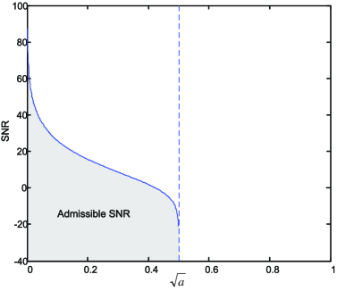
Figure 7: The shaded area is the region where treating interference as noise is optimal for obtaining the sum capacity of the symmetric Gaussian IC.

For a fixed $P$ and all $0\leq a\leq 1$, the upper bound in (IV-A) and the lower bound when receivers treat the interference as noise are plotted in Figure 8. We observe that up to a certain value of $a$, the upper bound coincides with the lower bound.

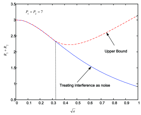
Figure 8: The upper bound obtained by solving (IV-A). The lower bound is obtained by treating the interference as noise.

IV-B New Outer Bound

For the weak Gaussian IC, there are two outer bounds that are tighter than the other known bounds. The first one, due to Kramer [12], is obtained by relying on the fact that the capacity region of the Gaussian IC is inside the capacity regions of the two underlying one-sided Gaussian ICs. Even though the capacity region of the one-sided Gaussian IC is unknown, there exists an outer bound for this channel that can be used instead. Kramers’ outer bound is the intersection of two regions $E_{1}$ and $E_{2}$. $E_{1}$ is the collection of all rate pairs $(R_{1},R_{2})$ satisfying

$$R_{1} \leq\gamma\left(\frac{(1-\beta)P^{\prime}}{\beta P^{\prime}+1/a}\right),$$ (149)

$$R_{2} \leq\gamma(\beta P^{\prime}),$$ (150)

for all $\beta\in[0,\beta_{\text{max}}]$, where $P^{\prime}=P_{1}/a+P_{2}$ and $\beta_{\text{max}}=\frac{P_{2}}{P^{\prime}(1+P_{1})}$. Similarly, $E_{2}$ is the collection of all rate pairs $(R_{1},R_{2})$ satisfying

$$R_{1} \leq\gamma(\alpha P^{\prime\prime}),$$ (151)

$$R_{2} \leq\gamma\left(\frac{(1-\alpha)P^{\prime\prime}}{\alpha P^{\prime\prime}+1/b}\right),$$ (152)

for all $\alpha\in[0,\alpha_{\text{max}}]$, where $P^{\prime\prime}=P_{1}+P_{2}/b$ and $\alpha_{\text{max}}=\frac{P_{1}}{P^{\prime\prime}(1+P_{2})}$.

The second outer bound, due to Etkin et al. [13], is obtained by using Genie aided technique to upper bound different linear combinations of rates that appear in the HK achievable region. Their outer bound is the union of all rate pairs $(R_{1},R_{2})$ satisfying

$$R_{1} \leq\gamma(P_{1}),$$ (153)

$$R_{2} \leq\gamma(P_{2}),$$ (154)

$$R_{1}+R_{2} \leq\gamma(P_{1})+\gamma\left(\frac{P_{2}}{1+bP_{1}}\right),$$ (155)

$$R_{1}+R_{2} \leq\gamma(P_{2})+\gamma\left(\frac{P_{1}}{1+aP_{2}}\right),$$ (156)

$$R_{1}+R_{2} \leq\gamma\left(aP_{2}+\frac{P_{1}}{1+bP_{1}}\right)+\gamma\left(bP_{1}+\frac{P_{2}}{1+aP_{2}}\right),$$ (157)

$$2R_{1}+R_{2} \leq\gamma(P_{1}+aP_{2})+\gamma\left(bP_{1}+\frac{P_{2}}{1+aP_{2}}\right)+0.5\log\left(\frac{1+P_{1}}{1+bP_{1}}\right),$$ (158)

$$R_{1}+2R_{2} \leq\gamma(bP_{1}+P_{2})+\gamma\left(aP_{2}+\frac{P_{1}}{1+bP_{1}}\right)+0.5\log\left(\frac{1+P_{2}}{1+aP_{2}}\right).$$ (159)

In the outer bound proposed here, we derive an upper bound on all linear combinations of the rates. Recall that to obtain the boundary points of the capacity region $\mathscr{C}$, it suffices to calculate $\sigma_{\mathscr{C}}(\mu,1)$ and $\sigma_{\mathscr{C}}(1,\mu)$ for all $1\leq\mu$. To this end, we make use of channels in A1 and B classes and channels in A2 and B classes to obtain upper bounds on $\sigma_{\mathscr{C}}(\mu,1)$ and $\sigma_{\mathscr{C}}(1,\mu)$, respectively.

In order to obtain an upper bound on $\sigma_{\mathscr{C}}(\mu,1)$, we introduce two optimization problems as follows. The first optimization problem is written as

$$W_{1}(\mu)= \min\frac{\mu_{1}}{2}\log\left[2\pi e(P_{1}+aP_{2}+1)\right]-\frac{\mu_{2}}{2}\log(2\pi e)+\frac{1}{2}\log\left(\frac{N_{21}}{N_{22}}+\frac{b^{\prime}P_{1}}{N_{22}}+\frac{P_{2}}{P_{2}+N_{22}}\right)$$

$$~{}~{}~{}~{}~{}~{}~{}~{}~{}~{}~{}~{}+\mu_{2}f_{h}\left(P_{1},1,N_{21},b^{\prime},\frac{1}{\mu_{2}}\right)+f_{h}(P_{2},N_{22},1,a,\mu_{1})$$

subject to:

$$~{}~{}~{}~{}~{}~{}~{}\mu_{1}+\mu_{2}=\mu$$

$$~{}~{}~{}~{}~{}~{}~{}b^{\prime}g_{2}=b$$

$$~{}~{}~{}~{}~{}~{}~{}b^{\prime}\leq N_{21}$$

$$~{}~{}~{}~{}~{}~{}~{}aN_{22}\leq 1$$

$$~{}~{}~{}~{}~{}~{}~{}(1-\sqrt{g_{2}})^{2}N_{22}+g_{2}N_{21}=1$$

$$~{}~{}~{}~{}~{}~{}~{}0\leq[\mu_{1},\mu_{2},b^{\prime},g_{2},N_{22},N_{21}].$$

In fact, the objective of the above minimization problem is an upper bound on the support function of a channel within Class A1 which is obtained in Lemma 3. The constraints are the combination of (80) and (81) which are applied to guarantee the admissibility of the channel and to validate the upper bound obtained in Lemma 3. Hence, $\sigma_{\mathscr{C}}(\mu,1)\leq W_{1}(\mu)$. By using a new variable $S=(1-\sqrt{g_{2}})^{2}N_{22}$, we obtain

$$W_{1}(\mu)= \min\frac{\mu_{1}}{2}\log\left[2\pi e(P_{1}+aP_{2}+1)\right]+\frac{1}{2}\log\left[(1-\sqrt{g_{2}})^{2}(\frac{1-S+bP_{1}}{g_{2}S}+\frac{P_{2}}{(1-\sqrt{g_{2}})^{2}P_{2}+S})\right]$$

$$~{}~{}~{}~{}~{}~{}~{}~{}~{}~{}~{}~{}+\mu_{2}f_{h}\left(P_{1},1,\frac{1-S}{g_{2}},\frac{b}{g_{2}},\frac{1}{\mu_{2}}\right)+f_{h}(P_{2},\frac{S}{(1-\sqrt{g_{2}})^{2}},1,a,\mu_{1})-\frac{\mu_{2}}{2}\log(2\pi e)$$

subject to:

$$~{}~{}~{}~{}~{}~{}~{}\mu_{1}+\mu_{2}=\mu$$

$$~{}~{}~{}~{}~{}~{}~{}S\leq 1-b$$

$$~{}~{}~{}~{}~{}~{}~{}S\leq\frac{(1-\sqrt{g_{2}})^{2}}{a}$$

$$~{}~{}~{}~{}~{}~{}~{}0\leq[\mu_{1},\mu_{2},S,g_{2}].$$

The second optimization problem is written as

$$W_{2}(\mu)= \min\mu\gamma\left(\frac{P_{1}}{N_{11}}+\frac{P_{1}}{a^{\prime}P_{2}+N_{12}}\right)+\gamma\left(\frac{P_{2}}{N_{22}}+\frac{P_{2}}{b^{\prime}P_{1}+N_{21}}\right)+f_{h}(P_{2},N_{22},N_{12},a^{\prime},\mu)$$

$$~{}~{}~{}~{}~{}~{}~{}~{}~{}~{}~{}~{}~{}+\frac{\mu}{2}\log((2\pi e)(a^{\prime}P_{2}+N_{12}))-\frac{1}{2}\log((2\pi e)(P_{2}+N_{22}))$$

subject to:

$$~{}~{}~{}~{}~{}~{}~{}a^{\prime}g_{1}=a$$

$$~{}~{}~{}~{}~{}~{}~{}b^{\prime}g_{2}=b$$

$$~{}~{}~{}~{}~{}~{}~{}b^{\prime}N_{11}\leq N_{21}$$

$$~{}~{}~{}~{}~{}~{}~{}a^{\prime}N_{22}\leq N_{12}$$

$$~{}~{}~{}~{}~{}~{}~{}(1-\sqrt{g_{1}})^{2}N_{11}+g_{1}N_{12}=1$$

$$~{}~{}~{}~{}~{}~{}~{}(1-\sqrt{g_{2}})^{2}N_{22}+g_{2}N_{21}=1$$

$$~{}~{}~{}~{}~{}~{}~{}0\leq[a^{\prime},b^{\prime},g_{1},g_{2},N_{11},N_{12},N_{22},N_{21}].$$

For this problem, Class B channels are used. In fact, the objective is the upper bound on the support function of channels within the class obtained in Lemma 5 and the constraints are defined to obtain the closed form formula for the upper bound and to confirm that the channels are admissible. Hence, we deduce $\sigma_{\mathscr{C}}(\mu,1)\leq W_{2}(\mu)$. By using new variables $S_{1}=g_{1}N_{12}$ and $S_{2}=g_{2}N_{21}$ , we obtain

$$W_{2}(\mu)= \min\mu\gamma\left(\frac{(1-\sqrt{g_{1}})^{2}P_{1}}{1-S_{1}}+\frac{g_{1}P_{1}}{aP_{2}+S_{1}}\right)+\gamma\left(\frac{(1-\sqrt{g_{2}})^{2}P_{2}}{1-S_{2}}+\frac{g_{2}P_{2}}{bP_{1}+S_{2}}\right)$$

$$~{}~{}~{}~{}~{}~{}~{}~{}~{}~{}~{}~{}~{}+f_{h}\left(P_{2},\frac{1-S_{2}}{(1-\sqrt{g_{2}})^{2}},\frac{S_{1}}{g_{1}},\frac{a}{g_{1}},\mu\right)+\frac{\mu}{2}\log\left((2\pi e)(\frac{aP_{2}+S_{1}}{g_{1}})\right)-\frac{1}{2}\log\left((2\pi e)(P_{2}+\frac{1-S_{2}}{(1-\sqrt{g_{2}})^{2}})\right)$$

subject to:

$$~{}~{}~{}~{}~{}~{}~{}\frac{b(1-S_{1})}{(1-\sqrt{g_{1}})^{2}}\leq S_{2}<1$$

$$~{}~{}~{}~{}~{}~{}~{}\frac{a(1-S_{2})}{(1-\sqrt{g_{2}})^{2}}\leq S_{1}<1$$

$$~{}~{}~{}~{}~{}~{}~{}0<[g_{1},g_{2}].$$

In a similar fashion, one can introduce two other optimization problems, say $\tilde{W}_{1}(\mu)$ and $\tilde{W}_{2}(\mu)$, to obtain upper bounds on $\sigma_{\mathscr{C}}(1,\mu)$ by using the upper bounds on the support functions of channels in Class A2 and Class B.

Theorem 6 (New Outer Bound)

For any rate pair $(R_{1},R_{2})$ achievable for the two-user weak Gaussian IC, the inequalities

$$\mu_{1}R_{1}+R_{2}\leq W(\mu_{1})=\min\{W_{1}(\mu_{1}),W_{2}(\mu_{1})\},$$ (164)

$$R_{1}+\mu_{2}R_{2}\leq\tilde{W}(\mu_{2})=\min\{\tilde{W}_{1}(\mu_{2}),\tilde{W}_{2}(\mu_{2})\},$$ (165)

hold for all $1\leq\mu_{1},\mu_{2}$.

To obtain an upper bound on the sum rate, we can apply the following inequality:

$$\mathscr{C}_{\text{sum}}\leq\min_{1\leq\mu_{1},\mu_{2}}\frac{(\mu_{2}-1)W(\mu_{1})+(\mu_{1}-1)\tilde{W}(\mu_{2})}{\mu_{1}\mu_{2}-1}.$$ (166)

IV-C Han-Kobayashi Achievable region

In this sub-section, we aim at characterizing $\mathscr{G}$ for the weak Gaussian IC. To this end, we first investigate some properties of $\mathscr{G}_{0}(P_{1},P_{2},\alpha,\beta)$. First of all, we show that none of the inequalities in describing $\mathscr{G}_{0}$ is redundant.

Figure 9: $\mathscr{G}_{0}$ for the weak Gaussian IC. $r_{1}$, $r_{2}$, $r_{3}$, and $r_{4}$ are extreme points of $\mathscr{G}_{0}$ in the interior of the first quadrant.

In Figure 9, all possible extreme points are shown. It is easy to prove that $r^{\prime}_{i}\notin\mathscr{G}_{0}$ for $i\in\{1,2,\ldots,6\}$. For instance, we consider $r^{\prime}_{6}=\left(\frac{2\psi_{4}-\psi_{5}}{3},\frac{2\psi_{5}-\psi_{4}}{3}\right)$. Since $\psi_{31}+\psi_{32}+\psi_{33}=\psi_{4}+\psi_{5}$ (see Section II.C), we have

$$\psi_{3} =\min\{\psi_{31},\psi_{32},\psi_{33}\}$$

$$\leq\frac{1}{3}(\psi_{31}+\psi_{32}+\psi_{33})$$

$$=\frac{1}{3}(\psi_{4}+\psi_{5}).$$

However, $\frac{1}{3}(\psi_{4}+\psi_{5})$ is the sum of the components of $r^{\prime}_{6}$. Therefore, $r^{\prime}_{6}$ violates (9) in the definition of the HK achievable region. Hence, $r^{\prime}_{6}\notin\mathscr{G}_{0}$. As another example, let us consider $r^{\prime}_{1}=(\psi_{1},\psi_{3}-\psi_{1})$. We claim that $r^{\prime}_{1}$ violates (10). To this end, we need to show that $\psi_{4}\leq\psi_{3}+\psi_{1}$. However, it is easy to see that $\psi_{4}\leq\psi_{31}+\psi_{1}$, $\psi_{4}\leq\psi_{32}+\psi_{1}$, and $\psi_{4}\leq\psi_{33}+\psi_{1}$ reduce to $0\leq(1-\alpha)(1-b+\beta(1-ab)P_{2})$, $0\leq(1-\beta)(1-a+(1-ab)P_{1})$, and $0\leq(1-\alpha)(1-\beta)aP_{2}$, respectively. Therefore, $r^{\prime}_{1}\notin\mathscr{G}_{0}$.

We conclude that $\mathscr{G}$ has four extreme points in the interior of the first quadrant, namely

$$r_{1} =(\psi_{1},\psi_{4}-2\psi_{1}),$$ (167)

$$r_{2} =(\psi_{4}-\psi_{3},2\psi_{3}-\psi_{4}),$$ (168)

$$r_{3} =(2\psi_{3}-\psi_{5},\psi_{5}-\psi_{3}),$$ (169)

$$r_{4} =(\psi_{5}-2\psi_{2},\psi_{2}).$$ (170)

Most importantly, $\mathscr{G}_{0}$ possesses the unique minimizer property. To prove this, we need to show that $\hat{\mathbf{y}}$, the minimizer of the optimization problem

$$\sigma_{D_{0}}(c_{1},c_{2},P_{1},P_{2},\alpha,\beta) =\max\{c_{1}R_{1}+c_{2}R_{2}|A\mathbf{R}\leq\Psi(P_{1},P_{2},\alpha,\beta)\}$$ (171)

$$=\min\{\mathbf{y}^{t}\Psi(P_{1},P_{2},\alpha,\beta)|A^{t}\mathbf{y}=(c_{1},c_{2})^{t},\mathbf{y}\geq 0\},$$

is independent of the parameters $P_{1}$, $P_{2}$, $\alpha$, and $\beta$ and only depends on $c_{1}$ and $c_{2}$. We first consider the case $(c_{1},c_{2})=(\mu,1)$ for all $1\leq\mu$. It can be shown that for $2<\mu$, the maximum of (171) is attained at $r_{1}$ regardless of $P_{1}$, $P_{2}$, $\alpha$, and $\beta$. Therefore, the dual program has the minimizer $\hat{\mathbf{y}}=(\mu-2,0,0,1,0)^{t}$ which is clearly independent of $P_{1}$, $P_{2}$, $\alpha$, and $\beta$. In this case, we have

$$\sigma_{D_{0}}(\mu,1,P_{1},P_{2},\alpha,\beta)=(\mu-2)\psi_{1}+\psi_{4},~{}2<\mu.$$ (172)

For $1\leq\mu\leq 2$, one can show that $r_{2}$ and $\hat{\mathbf{y}}=(0,0,2-\mu,\mu-1,0)^{t}$ are the maximizer and the minimizer of (171), respectively. In this case, we have

$$\sigma_{D_{0}}(\mu,1,P_{1},P_{2},\alpha,\beta)=(2-\mu)\psi_{3}+(\mu-1)\psi_{4},~{}1\leq\mu\leq 2.$$ (173)

Next, we consider the case $(c_{1},c_{2})=(1,\mu)$ for all $1\leq\mu$. Again, it can be shown that for $2<\mu$ and $1\leq\mu\leq 2$, $\hat{\mathbf{y}}=(0,\mu-2,0,0,1)^{t}$ and $\hat{\mathbf{y}}=(0,0,2-\mu,0,\mu-1)^{t}$ minimizes (171), respectively. Hence, we have

$$\sigma_{D_{0}}(1,\mu,P_{1},P_{2},\alpha,\beta) =(\mu-2)\psi_{2}+\psi_{5}, ~{}\text{if}~{}2<\mu,$$ (174)

$$\sigma_{D_{0}}(1,\mu,P_{1},P_{2},\alpha,\beta) =(2-\mu)\psi_{3}+(\mu-1)\psi_{5}, ~{}\text{if}~{}1\leq\mu\leq 2.$$ (175)

We conclude that the solutions of the dual program are always independent of $P_{1}$, $P_{2}$, $\alpha$, and $\beta$. Hence, $\mathscr{G}_{0}$ possesses the unique minimizer property.

Theorem 7

For the two-user weak Gaussian IC, time-sharing and concavification result in the same region. In other words, $\mathscr{G}$ can be fully characterized by using TD/FD and allocating power over three different dimensions.

Proof:

Since $\mathscr{G}_{0}$ possesses the unique minimizer property, from Theorem 1, we deduce that $\mathscr{G}=\mathscr{G}_{2}$. Moreover, using Theorem 3, the number of frequency bands is at most three. ∎

To obtain the support function of $\mathscr{G}_{2}$, we need to obtain $g(c_{1},c_{2},P_{1},P_{2},\alpha,\beta)$ defined in (II-D). Since $\mathscr{G}_{0}$ possesses the unique minimizer property, (II-D) can be simplified. Let us consider the case where $(c_{1},c_{2})=(\mu,1)$ for $\mu>2$. It can be shown that for this case

$$g=\max_{(\alpha,\beta)\in[0,1]^{2}}(\mu-2)\psi_{1}(P_{1},P_{2},\alpha,\beta)+\psi_{4}(P_{1},P_{2},\alpha,\beta).$$ (176)

Substituting into (II-D), we obtain

$$\sigma_{\mathscr{G}_{2}}(\mu,1,P_{1},P_{2})= \max\sum_{i=1}^{3}\lambda_{i}\left[(\mu-2)\psi_{1}(P_{1i},P_{2i},\alpha_{i},\beta_{i})+\psi_{4}(P_{1i},P_{2i},\alpha_{i},\beta_{i})\right]$$

subject to:

$$~{}~{}~{}~{}~{}~{}~{}\sum_{i=1}^{3}\lambda_{i}=1$$

$$~{}~{}~{}~{}~{}~{}~{}\sum_{i=1}^{3}\lambda_{i}P_{1i}\leq P_{1}$$

$$~{}~{}~{}~{}~{}~{}~{}\sum_{i=1}^{3}\lambda_{i}P_{2i}\leq P_{2}$$

$$~{}~{}~{}~{}~{}~{}~{}0\leq\lambda_{i},0\leq P_{1i},0\leq P_{2i},~{}\forall i\in\{1,2,3\}$$

$$~{}~{}~{}~{}~{}~{}~{}0\leq\alpha_{i}\leq 1,0\leq\beta_{i}\leq 1,~{}\forall i\in\{1,2,3\}.$$

For other ranges of $(c_{1},c_{2})$, a similar optimization problem can be formed. It is worth noting that even though the number of parameters in characterizing $\mathscr{G}$ is reduced, it is still prohibitively difficult to characterize boundary points of $\mathscr{G}$. In Figures (10) and (11), different bounds for the symmetric weak Gaussian IC are plotted. As shown in these figures, the new outer bound is tighter than the previously known bounds.

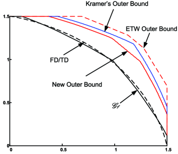
Figure 10: Comparison between different bounds for the symmetric weak Gaussian IC when $P=7$ and $a=0.2$.

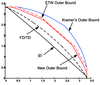
Figure 11: Comparison between different bounds for the symmetric weak Gaussian IC when $P=100$ and $a=0.1$.

V One-sided Gaussian Interference Channels

Throughout this section, we consider the one-sided Gaussian IC obtained by setting $b=0$, i.e, the second receiver incurs no interference from the first transmitter. One can further split the class of one-sided ICs into two subclasses: the strong one-sided IC and the weak one-sided IC. For the former, $a\geq 1$ and the capacity region is fully characterized [16]. In this case, the capacity region is the union of all rate pairs $(R_{1},R_{2})$ satisfying

$$R_{1} \leq\gamma{(P_{1})},$$

$$R_{2} \leq\gamma(P_{2}),$$

$$R_{1}+R_{2} \leq\gamma(P_{1}+aP_{2}).$$

For the latter, $a<1$ and the full characterization of the capacity region is still an open problem. Therefore, we always assume $a<1$. Three important results are proved for this channel. The first one, proved by Costa in [11], states that the capacity region of the weak one-sided IC is equivalent to that of the degraded IC with an appropriate change of parameters. The second one, proved by Sato in [10], states that the capacity region of the degraded Gaussian IC is outer bounded by the capacity region of a certain degraded broadcast channel. The third one, proved by Sason in [16], characterizes the sum capacity by combining Costa’s and Sato’s results.

In this section, we provide an alternative proof for the outer bound obtained by Sato. We then characterize the full HK achievable region where Gaussian codebooks are used, i.e., $\mathscr{G}$.

V-A Sum Capacity

For the sake of completeness, we first state the sum capacity result obtained by Sason.

Theorem 8 (Sason)

The rate pair $\left(\gamma\left(\frac{P_{1}}{1+aP_{2}}\right),\gamma(P_{2})\right)$ is an extreme point of the capacity region of the one-sided Gaussian IC. Moreover, the sum capacity of the channel is attained at this point.

V-B Outer Bound

In [10], Sato derived an outer bound on the capacity of the degraded IC. This outer bound can be used for the weak one-sided IC as well. This is due to Costa’s result which states that the capacity region of the degraded Gaussian IC is equivalent to that of the weak one-sided IC with an appropriate change of parameters.

Theorem 9 (Sato)

If the rate pair $(R_{1},R_{2})$ belongs to the capacity region of the weak one-sided IC, then it satisfies

$$\begin{array}[]{ll}R_{1}&\leq\gamma{\left(\frac{(1-\beta)P}{1/a+\beta P}\right)},\\ R_{2}&\leq\gamma{(\beta P)},\end{array}$$ (178)

for all $\beta\in[0,1]$ where $P=P_{1}/a+P_{2}$.

Proof:

Since the sum capacity is attained at the point where User 2 transmits at its maximum rate $R_{2}=\gamma(P_{2})$, other boundary points of the capacity region can be obtained by characterizing the solutions of $\sigma_{\mathscr{C}}(\mu,1)=\max\left\{\mu R_{1}+R_{2}|(R_{1},R_{2})\in\mathscr{C}\right\}$ for all $1\leq\mu$. Using Fano’s inequality, we have

$$n(\mu R_{1}+R_{2})\stackrel{{\scriptstyle}}{{\leq}} \mu I(x_{1}^{n};y_{1}^{n})+I(x_{2}^{n};y_{2}^{n})+n\epsilon_{n}$$

$$\stackrel{{\scriptstyle}}{{=}} \mu h(y_{1}^{n})-\mu h(y_{1}^{n}|x_{1}^{n})+h(y_{2}^{n})-h(y_{2}^{n}|x_{2}^{n})+n\epsilon_{n}$$

$$\stackrel{{\scriptstyle}}{{=}} [\mu h(x_{1}^{n}+\sqrt{a}x_{2}^{n}+z_{1}^{n})-h(z_{2}^{n})]+[h(x_{2}^{n}+z_{2}^{n})-\mu h(\sqrt{a}x_{2}^{n}+z_{1}^{n})]+n\epsilon_{n}$$

$$\stackrel{{\scriptstyle(a)}}{{\leq}} \frac{\mu n}{2}\log\left[2\pi e(P_{1}+aP_{2}+1)\right]-\frac{n}{2}\log(2\pi e)+[h(x_{2}^{n}+z_{2}^{n})-\mu h(\sqrt{a}x_{2}^{n}+z_{1}^{n})]+n\epsilon_{n}$$

$$\stackrel{{\scriptstyle(b)}}{{\leq}} \frac{\mu n}{2}\log\left[2\pi e(P_{1}+aP_{2}+1)\right]-\frac{n}{2}\log(2\pi e)+nf_{h}(P_{2},1,1,a,\mu)+n\epsilon_{n},$$

where (a) follows from the fact that Gaussian distribution maximizes the differential entropy for a given constraint on the covariance matrix and (b) follows from the definition of $f_{h}$ in (61).

Depending on the value of $\mu$, we consider the following two cases:

1- For $1\leq\mu\leq\frac{P_{2}+1/a}{P_{2}+1}$, we have

$$\mu R_{1}+R_{2}\leq\mu\gamma\left(\frac{P_{1}}{1+aP_{2}}\right)+\gamma(P_{2}).$$ (179)

In fact, the point $\left(\gamma\left(\frac{P_{1}}{1+aP_{2}}\right),\gamma(P_{2})\right)$ which is achievable by treating interference as noise at Receiver 1, satisfies (179) with equality. Therefore, it belongs to the capacity region. Moreover, by setting $\mu=1$, we deduce that this point corresponds to the sum capacity of the one-sided Gaussian IC. This is in fact an alternative proof for Sason’s result.

2- For $\frac{P_{2}+1/a}{P_{2}+1}<\mu\leq\frac{1}{a}$, we have

$$\mu R_{1}+R_{2}\leq\frac{\mu}{2}\log\left(P_{1}+aP_{2}+1\right)+\frac{1}{2}\log\left(\frac{1/a-1}{\mu-1}\right)-\frac{\mu}{2}\log\left(\frac{a\mu(1/a-1)}{\mu-1}\right).$$ (180)

Equivalently, we have

$$\mu R_{1}+R_{2}\leq\frac{\mu}{2}\log\left(\frac{(aP+1)(\mu-1)}{\mu(1-a)}\right)+\frac{1}{2}\log\left(\frac{1/a-1}{\mu-1}\right),$$ (181)

where $P=P_{1}/a+P_{2}$. Let us define $E_{1}$ as the set of all rate pairs $(R_{1},R_{2})$ satisfying (181), i.e.

$$E_{1}=\left\{(R_{1},R_{2})|\mu R_{1}+R_{2}\leq\frac{\mu}{2}\log\left(\frac{(aP+1)(\mu-1)}{\mu(1-a)}\right)+\frac{1}{2}\log\left(\frac{1/a-1}{\mu-1}\right),~{}\forall\frac{P_{2}+1/a}{P_{2}+1}<\mu\leq\frac{1}{a}\right\}.$$ (182)

We claim that $E_{1}$ is the dual representation of the region defined in the statement of the theorem, see (6). To this end, we define $E_{2}$ as

$$E_{2}=\left\{(R_{1},R_{2})|R_{1}\leq\gamma{\left(\frac{(1-\beta)P}{1/a+\beta P}\right)},R_{2}\leq\gamma{(\beta P)},~{}\forall\beta\in[0,1]\right\}$$ (183)

We evaluate the support function of $E_{2}$ as

$$\sigma_{E_{2}}(\mu,1)=\max\left\{\mu R_{1}+R_{2}|(R_{1},R_{2})\in E_{2}\right\}.$$ (184)

It is easy to show that $\beta=\frac{1/a-1}{P(\mu-1)}$ maximizes the above optimization problem. Therefore, we have

$$\sigma_{E_{2}}(\mu,1)=\frac{\mu}{2}\log\left(\frac{(aP+1)(\mu-1)}{\mu(1-a)}\right)+\frac{1}{2}\log\left(\frac{1/a-1}{\mu-1}\right).$$ (185)

Since $E_{2}$ is a closed convex set, we can use (6) to obtain its dual representation which is indeed equivalent to (182). This completes the proof. ∎

V-C Han-Kobayashi Achievable Region

In this subsection, we characterize $\mathscr{G}_{0}$, $\mathscr{G}_{1}$, $\mathscr{G}_{2}$, and $\mathscr{G}$ for the weak one-sided Gaussian IC. $\mathscr{G}_{0}$ can be characterized as follows. Since there is no link between Transmitter 1 and Receiver 2, User 1’s message in the HK achievable region is only the private message, i.e., $\alpha=1$. In this case, we have

$$\psi_{1} =\gamma\left(\frac{P_{1}}{1+a\beta P_{2}}\right),$$ (186)

$$\psi_{2} =\gamma(P_{2}),$$ (187)

$$\psi_{31} =\gamma\left(\frac{P_{1}+a(1-\beta)P_{2}}{1+a\beta P_{2}}\right)+\gamma(\beta P_{2}),$$ (188)

$$\psi_{32} =\gamma\left(\frac{P_{1}}{1+a\beta P_{2}}\right)+\gamma(P_{2}),$$ (189)

$$\psi_{33} =\gamma\left(\frac{P_{1}+a(1-\beta)P_{2}}{1+a\beta P_{2}}\right)+\gamma(\beta P_{2}),$$ (190)

$$\psi_{4} =\gamma\left(\frac{P_{1}+a(1-\beta)P_{2}}{1+a\beta P_{2}}\right)+\gamma\left(\frac{P_{1}}{1+a\beta P_{2}}\right)+\gamma(\beta P_{2}),$$ (191)

$$\psi_{5} =\gamma(\beta P_{2})+\gamma(P_{2})+\gamma\left(\frac{P_{1}+a(1-\beta)P_{2}}{1+a\beta P_{2}}\right),$$ (192)

It is easy to show that $\psi_{3}=\min\{\psi_{31},\psi_{32},\psi_{33}\}=\psi_{31}$, $\psi_{31}+\psi_{1}=\psi_{4}$, $\psi_{31}+\psi_{2}=\psi_{5}$. Hence, $\mathscr{G}_{0}$ can be represented as all rate pairs $(R_{1},R_{2})$ satisfying

$$R_{1} \leq\gamma\left(\frac{P_{1}}{1+a\beta P_{2}}\right),$$ (193)

$$R_{2} \leq\gamma(P_{2}),$$ (194)

$$R_{1}+R_{2} \leq\gamma\left(\frac{P_{1}+a(1-\beta)P_{2}}{1+a\beta P_{2}}\right)+\gamma(\beta P_{2}).$$ (195)

We claim that $\mathscr{G}_{2}=\mathscr{G}$. To prove this, we need to show that $\mathscr{G}_{0}$ possesses the unique minimizer property. $\mathscr{G}_{0}$ is a pentagon with two extreme points in the interior of the first quadrant, namely $r_{1}$ and $r_{2}$ where

$$r_{1} =\left(\gamma\left(\frac{P_{1}}{1+a\beta P_{2}}\right),\gamma{\left(\frac{(1-\beta)aP_{2}}{1+P_{1}+\beta aP_{2}}\right)}+\gamma(\beta P_{2})\right),$$ (196)

$$r_{2} =\left(\gamma\left(\frac{P_{1}+a(1-\beta)P_{2}}{1+a\beta P_{2}}\right)+\gamma(\beta P_{2})-\gamma(P_{2}),\gamma(P_{2})\right).$$ (197)

Using above, it can be verified that $\mathscr{G}_{0}$ possesses the unique minimizer property.

Next, we can use the optimization problem in (II-D) to obtain the support function of $\mathscr{G}$. However, we only need to consider $(c_{1},c_{2})=(\mu,1)$ for $\mu>1$. Therefore, we have

$$g(\mu,1,P_{1},P_{2},\beta)=\max_{0\leq\beta\leq 1}\mu\gamma{\left(\frac{P_{1}}{1+\beta aP_{2}}\right)}+\gamma{(\beta P_{2})}+\gamma{\left(\frac{(1-\beta)aP_{2}}{1+P_{1}+\beta aP_{2}}\right)}.$$ (198)

Substituting into (II-D), we conclude that boundary points of $\mathscr{G}$ can be characterized by solving the following optimization problem:

$$W= \max\sum_{i=1}^{3}\lambda_{i}\left[\mu\gamma{\left(\frac{P_{1i}}{1+\beta_{i}aP_{2i}}\right)}+\gamma{(\beta_{i}P_{2i})}+\gamma{\left(\frac{(1-\beta_{i})aP_{2i}}{1+P_{1i}+\beta_{i}aP_{2i}}\right)}\right]$$

subject to:

$$~{}~{}~{}~{}~{}~{}~{}\sum_{i=1}^{3}\lambda_{i}=1$$

$$~{}~{}~{}~{}~{}~{}~{}\sum_{i=1}^{3}\lambda_{i}P_{1i}\leq P_{1}$$

$$~{}~{}~{}~{}~{}~{}~{}\sum_{i=1}^{3}\lambda_{i}P_{2i}\leq P_{2}$$

$$~{}~{}~{}~{}~{}~{}~{}0\leq\beta_{i}\leq 1,~{}\forall i\in\{1,2,3\}$$

$$~{}~{}~{}~{}~{}~{}~{}0\leq[P_{1i},P_{2i},\lambda_{i}],~{}\forall i\in\{1,2,3\}.$$

For the sake of completeness, we provide a simple description for $\mathscr{G}_{1}$ in the next lemma.

Lemma 7

The region $\mathscr{G}_{1}$ can be represented as the collection of all rate pairs $(R_{1},R_{2})$ satisfying

$$R_{1} \leq\gamma{\left(\frac{P_{1}}{1+a\beta^{\prime}P_{2}}\right)},$$ (200)

$$R_{2} \leq\gamma{(\beta^{\prime}P_{2})}+\gamma{\left(\frac{a(1-\beta^{\prime})P_{2}}{1+P_{1}+a\beta^{\prime}P_{2}}\right)},$$ (201)

for all $\beta^{\prime}\in[0,1]$. Moreover, $\mathscr{G}_{1}$ is convex and any point that lies on its boundary can be achieved by using superposition coding and successive decoding.

Proof:

Let $E$ denote the set defined in the above lemma. It is easy to show that $E$ is convex and $E\subseteq\mathscr{G}_{1}$. To prove the inverse inclusion, it suffices to show that the extreme points of $\mathscr{G}_{0}$, $r_{1}$ and $r_{2}$ (see (196) and (197)) are inside $E$ for all $\beta\in[0,1]$. By setting $\beta^{\prime}=\beta$, we see that $r_{1}\in E$. To prove $r_{2}\in E$, we set $\beta^{\prime}=1$. We conclude that $r_{2}\in E$ if the following inequality holds

$$\gamma\left(\frac{P_{1}+a(1-\beta)P_{2}}{1+a\beta P_{2}}\right)+\gamma(\beta P_{2})-\gamma(P_{2})\leq\gamma{\left(\frac{P_{1}}{1+aP_{2}}\right)},$$ (202)

for all $\beta\in[0,1]$. However, (202) reduces to $0\leq(1-a)(1-\beta)P_{2}$ which holds for all $\beta\in[0,1]$. Hence, $\mathscr{G}_{1}\subseteq E$. Using these facts, it is straightforward to show that the boundary points $\mathscr{G}_{1}$ are achievable by using superposition coding and successive decoding. ∎

Figure 12 compares different bounds for the one-sided Gaussian IC.

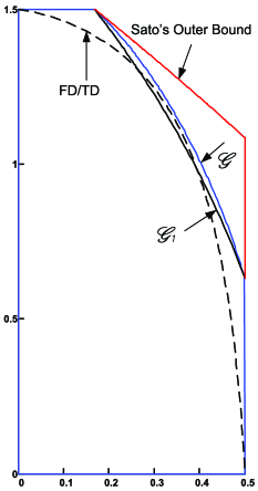
Figure 12: Comparison between different bounds for the one-sided Gaussian IC when $P_{1}=1$, $P_{2}=7$, and $a=0.4$.

VI Mixed Gaussian Interference Channels

In this section, we focus on the mixed Gaussian Interference channel. We first characterize the sum capacity of this channel. Then, we provide an outer bound on the capacity region. Finally, we investigate the HK achievable region. Without loss of generality, we assume $a<1$ and $b\geq 1$.

VI-A Sum Capacity

Theorem 10

The sum capacity of the mixed Gaussian IC with $a<1$ and $b\geq 1$ can be stated as

$$\mathscr{C}_{sum}=\gamma\left(P_{2}\right)+\min\left\{\gamma\left(\frac{P_{1}}{1+aP_{2}}\right),\gamma\left(\frac{bP_{1}}{1+P_{2}}\right)\right\}.$$ (203)

Proof:

We need to prove the achievability and converse for the theorem.

Achievability part: Transmitter 1 sends a common message to both receivers, while the first user’s signal is considered as noise at both receivers. In this case, the rate

$$R_{1}=\min\left\{\gamma\left(\frac{P_{1}}{1+aP_{2}}\right),\gamma\left(\frac{bP_{1}}{1+P_{2}}\right)\right\}$$ (204)

is achievable. At Receiver 2, the signal from Transmitter 1 can be decoded and removed. Therefore, User 2 is left with a channel without interference and it can communicate at its maximum rate which is

$$R_{2}=\gamma(P_{2}).$$ (205)

By adding (204) and (205), we obtain the desired result.

Converse part: The sum capacity of the Gaussian IC is upper bounded by that of the two underlying one-sided Gaussian ICs. Hence, we can obtain two upper bounds on the sum rate. We first remove the interfering link between Transmitter 1 and Receiver 2. In this case, we have a one-sided Gaussian IC with weak interference. The sum capacity of this channel is known [16]. Hence, we have

$$\mathscr{C}_{sum}\leq\gamma(P_{2})+\gamma\left(\frac{P_{1}}{1+aP_{2}}\right).$$ (206)

By removing the interfering link between Transmitter 2 and Receiver 1, we obtain a one-sided Gaussian IC with strong interference. The sum capacity of this channel is known. Hence, we have

$$\mathscr{C}_{sum}\leq\gamma\left(bP_{1}+P_{2}\right),$$ (207)

which equivalently can be written as

$$\mathscr{C}_{sum}\leq\gamma(P_{2})+\gamma\left(\frac{bP_{1}}{1+P_{2}}\right).$$ (208)

By taking the minimum of the right hand sides of (206) and (208), we obtain

$$\mathscr{C}_{sum}\leq\gamma\left(P_{2}\right)+\min\left\{\gamma\left(\frac{P_{1}}{1+aP_{2}}\right),\gamma\left(\frac{bP_{1}}{1+P_{2}}\right)\right\}.$$ (209)

This completes the proof. ∎

Remark 4

In an independent work [25], the sum capacity of the mixed Gaussian IC is obtained for a certain range of parameters, whereas in the above theorem, we characterize the sum capacity of this channel for the entire range of its parameters (see also [24]).

By comparing $\gamma\left(\frac{P_{1}}{1+aP_{2}}\right)$ with $\gamma\left(\frac{bP_{1}}{1+P_{2}}\right)$, we observe that if $1+P_{2}\leq b+abP_{2}$, then the sum capacity corresponds to the sum capacity of the one-sided weak Gaussian IC, whereas if $1+P_{2}>b+abP_{2}$, then the sum capacity corresponds to the sum capacity of the one-sided strong IC. Similar to the one-sided Gaussian IC, since the sum capacity is attained at the point where User 2 transmits at its maximum rate $R_{2}=\gamma(P_{2})$, other boundary points of the capacity region can be obtained by characterizing the solutions of $\sigma_{\mathscr{C}}(\mu,1)=\max\left\{\mu R_{1}+R_{2}|(R_{1},R_{2})\in\mathscr{C}\right\}$ for all $1\leq\mu$.

VI-B New Outer Bound

The best outer bound to date, due to Etkin et al. [13], is obtained by using the Genie aided technique. This bound is the union of all rate pairs $(R_{1},R_{2})$ satisfying

$$R_{1} \leq\gamma(P_{1}),$$ (210)

$$R_{2} \leq\gamma(P_{2}),$$ (211)

$$R_{1}+R_{2} \leq\gamma(P_{2})+\gamma\left(\frac{P_{1}}{1+aP_{2}}\right),$$ (212)

$$R_{1}+R_{2} \leq\gamma(P_{2}+bP_{1}),$$ (213)

$$2R_{1}+R_{2} \leq\gamma(P_{1}+aP_{2})+\gamma\left(bP_{1}+\frac{P_{2}}{1+aP_{2}}\right)+\gamma\left(\frac{P_{1}}{1+bP_{1}}\right).$$ (214)

The capacity region of the mixed Gaussian IC is inside the intersection of the capacity regions of the two underlying one-sided Gaussian ICs. Removing the link between Transmitter 1 and Receiver 2 results in a weak one-sided Gaussian IC whose outer bound $E_{1}$ is the collection of all rate pairs $(R_{1},R_{2})$ satisfying

$$R_{1} \leq\gamma\left(\frac{(1-\beta)P^{\prime}}{\beta P^{\prime}+1/a}\right),$$ (215)

$$R_{2} \leq\gamma(\beta P^{\prime}),$$ (216)

for all $\beta\in[0,\beta_{\text{max}}]$, where $P^{\prime}=P_{1}/a+P_{2}$ and $\beta_{\text{max}}=\frac{P_{2}}{P^{\prime}(1+P_{1})}$. On the other hand, removing the link between Transmitter 2 and Receiver 1 results in a strong one-sided Gaussian IC whose capacity region $E_{2}$ is fully characterized as the collection of all rate pairs $(R_{1},R_{2})$ satisfying

$$R_{1} \leq\gamma(bP_{1}),$$ (217)

$$R_{2} \leq\gamma\left(P_{2}\right),$$ (218)

$$R_{1}+R_{2} \leq\gamma(bP_{1}+P_{2}).$$ (219)

Using the channels in Class C, we upper bound $\sigma_{\mathscr{C}}(\mu,1)$ based on the following optimization problem:

$$W(\mu)= \min\frac{\mu-1}{2}\log\left(2\pi e(P_{1}+aP_{2}+1)\right)+\frac{1}{2}\log\left(2\pi e\left(\frac{P_{2}N_{22}}{P_{2}+N_{22}}+b^{\prime}P_{1}+N_{21}\right)\right)$$

$$~{}~{}~{}~{}~{}~{}~{}-\frac{1}{2}\log(2\pi eN_{21})-\frac{1}{2}\log(2\pi eN_{22})+f_{h}(P_{2},N_{22},1,a,\mu-1)$$

subject to:

$$~{}~{}~{}~{}~{}~{}~{}b^{\prime}g_{2}=b$$

$$~{}~{}~{}~{}~{}~{}~{}b^{\prime}\geq N_{21}$$

$$~{}~{}~{}~{}~{}~{}~{}aN_{22}\leq 1$$

$$~{}~{}~{}~{}~{}~{}~{}(1-\sqrt{g_{2}})^{2}N_{22}+g_{2}N_{21}=1$$

$$~{}~{}~{}~{}~{}~{}~{}0\leq[b^{\prime},g_{2},N_{22},N_{21}].$$

By substituting $S=g_{2}N_{21}$, we obtain

$$W(\mu)= \min\frac{\mu-1}{2}\log\left(2\pi e(P_{1}+aP_{2}+1)\right)+\frac{1}{2}\log\left(2\pi e\left(\frac{P_{2}(1-S)}{(1-\sqrt{g_{2}})^{2}P_{2}+1-S}+\frac{bP_{1}+S}{g_{2}}\right)\right)$$

$$~{}~{}~{}~{}~{}~{}~{}-\frac{1}{2}\log\left(\frac{2\pi eS}{g_{2}}\right)-\frac{1}{2}\log\left(\frac{2\pi e(1-S)}{(1-\sqrt{g_{2}})^{2}}\right)+f_{h}\left(P_{2},\frac{1-S}{(1-\sqrt{g_{2}})^{2}},1,a,\mu-1\right)$$

subject to:

$$~{}~{}~{}~{}~{}~{}~{}S<1$$

$$~{}~{}~{}~{}~{}~{}~{}a(1-S)\leq(1-\sqrt{g_{2}})^{2}$$

$$~{}~{}~{}~{}~{}~{}~{}0\leq[S,g_{2}].$$

Hence, we have the following theorem that provides an outer bound on the capacity region of the mixed Gaussian IC.

Theorem 11

For any rate pair $(R_{1},R_{2})$ achievable for the two-user mixed Gaussian IC, $(R_{1},R_{2})\in E_{1}\bigcap E_{2}$. Moreover, the inequality

$$\mu R_{1}+R_{2}\leq W(\mu)$$ (222)

holds for all $1\leq\mu$.

VI-C Han-Kobayashi Achievable Region

In this subsection, we study the HK achievable region for the mixed Gaussian IC. Since Receiver 2 can always decode the message of the first user, User 1 associates all its power to the common message. User 2, on the other hand, allocates $\beta P_{2}$ and $(1-\beta)P_{2}$ of its total power to its private and common messages, respectively, where $\beta\in[0,1]$. Therefore, we have

$$\psi_{1} =\gamma\left(\frac{P_{1}}{1+a\beta P_{2}}\right),$$ (223)

$$\psi_{2} =\gamma(P_{2}),$$ (224)

$$\psi_{31} =\gamma\left(\frac{P_{1}+a(1-\beta)P_{2}}{1+a\beta P_{2}}\right)+\gamma(\beta P_{2}),$$ (225)

$$\psi_{32} =\gamma(P_{2}+bP_{1}),$$ (226)

$$\psi_{33} =\gamma\left(\frac{a(1-\beta)P_{2}}{1+a\beta P_{2}}\right)+\gamma(\beta P_{2}+bP_{1}),$$ (227)

$$\psi_{4} =\gamma\left(\frac{P_{1}+a(1-\beta)P_{2}}{1+a\beta P_{2}}\right)+\gamma(\beta P_{2}+bP_{1}),$$ (228)

$$\psi_{5} =\gamma(\beta P_{2})+\gamma(P_{2}+bP_{1})+\gamma\left(\frac{a(1-\beta)P_{2}}{1+a\beta P_{2}}\right).$$ (229)

Figure 13: The new region $\mathscr{G}^{\prime}_{0}$ which is obtained by enlarging $\mathscr{G}_{0}$.

Due to the fact that the sum capacity is attained at the point where the second user transmits at its maximum rate, the last inequality in the description of the HK achievable region can be removed. Although the point $r^{\prime}_{5}=(\psi_{3}-\gamma(P_{2}),\gamma(P_{1}))$ in Figure 9 may not be in $\mathscr{G}_{0}$, this point is always achievable due to the sum capacity result. Hence, we can enlarge $\mathscr{G}_{0}$ by removing $r_{3}$ and $r_{4}$. Let us denote the resulting region as $\mathscr{G}^{\prime}_{0}$. Moreover, one can show that $r^{\prime}_{2}$, $r^{\prime}_{3}$, $r^{\prime}_{4}$, and $r^{\prime}_{6}$ are still outside $\mathscr{G}^{\prime}_{0}$. However, for the mixed Gaussian IC, it is possible that $r^{\prime}_{1}$ belongs to $\mathscr{G}^{\prime}_{0}$. In Figure 13, two alternative cases for the region $\mathscr{G}^{\prime}_{0}$ along with the new labeling of its extreme points are plotted. The new extreme points can be written as

$$r_{1} =(\psi_{1},\psi_{4}-2\psi_{1}),$$

$$r_{2} =(\psi_{1},\psi_{3}-\psi_{1}),$$

$$r_{3} =(\psi_{4}-\psi_{3},2\psi_{3}-\psi_{4}),$$

$$r_{4} =(\psi_{3}-\psi_{2},\psi_{2}).$$

In fact, we have either $\mathscr{G}^{\prime}_{0}=\text{conv}\{r_{1},r_{3},r_{4}\}$ or $\mathscr{G}^{\prime}_{0}=\text{conv}\{r_{2},r_{4}\}$.

To simplify the characterization of $\mathscr{G}_{1}$, we consider three cases:

Case I:

$1+P_{2}\leq b+abP_{2}$.

Case II:

$1+P_{2}>b+abP_{2}$ and $1-a\leq abP_{1}$.

Case III:

$1+P_{2}>b+abP_{2}$ and $1-a>abP_{1}$.

Case I ($1+P_{2}\leq b+abP_{2}$): In this case, $\psi_{3}=\psi_{31}$. Moreover, it is easy to verify that $\psi_{31}+\psi_{1}\leq\psi_{4}$ which means (10) is redundant for the entire range of parameters. Hence, $\mathscr{G}^{\prime}_{0}=\text{conv}\{r_{2},r_{4}\}$ consists of all rate pairs $(R_{1},R_{2})$ satisfying

$$R_{1} \leq\gamma\left(\frac{P_{1}}{1+a\beta P_{2}}\right),$$ (230)

$$R_{2} \leq\gamma\left(P_{2}\right),$$ (231)

$$R_{1}+R_{2} \leq\gamma\left(\frac{P_{1}+a(1-\beta)P_{2}}{1+a\beta P_{2}}\right)+\gamma(\beta P_{2}),$$ (232)

where $\beta\in[0,1]$. Using a reasoning similar to the one used to express boundary points of $\mathscr{G}_{1}$ for the one-sided Gaussian IC, we can express boundary points of $\mathscr{G}_{1}$ as

$$R_{1} \leq\gamma\left(\frac{P_{1}}{1+a\beta P_{2}}\right),$$ (233)

$$R_{2} \leq\gamma(\beta P_{2})+\gamma\left(\frac{a(1-\beta)P_{2}}{1+P_{1}+a\beta P_{2}}\right),$$ (234)

for all $\beta\in[0,1]$.

Theorem 12

For the mixed Gaussian IC satisfying $1\leq ab$, region $\mathscr{G}$ is equivalent to that of the one sided Gaussian IC obtained from removing the interfering link between Transmitter 1 and Receiver 2.

Proof:

If $1\leq ab$, then $1+P_{2}\leq b+abP_{2}$ holds for all $P_{1}$ and $P_{2}$. Hence, $\mathscr{G}^{\prime}_{0}(P_{1},P_{2},\beta)$ is a pentagon defined by (230), (231), and (231). Comparing with the corresponding region for the one-sided Gaussian IC, we see that $\mathscr{G}^{\prime}_{0}$ is equivalent to $\mathscr{G}_{0}$ obtained for the one-sided Gaussian IC. This directly implies that $\mathscr{G}$ is the same for both channels. ∎

Case II ($1+P_{2}>b+abP_{2}$ and $1-a\leq abP_{1}$): In this case, $\psi_{3}=\min\{\psi_{31},\psi_{32}\}$. It can be shown that $\mathscr{G}_{1}$ is the union of three regions $E_{1}$, $E_{2}$, and $E_{3}$, i.e, $\mathscr{G}_{0}=E_{1}\bigcup E_{2}\bigcup E_{3}$. Region $E_{1}$ is the union of all rate pairs $(R_{1},R_{2})$ satisfying

$$R_{1} \leq\gamma\left(\frac{P_{1}}{1+a\beta P_{2}}\right),$$ (235)

$$R_{2} \leq\gamma(\beta P_{2})+\gamma\left(\frac{a(1-\beta)P_{2}}{1+P_{1}+a\beta P_{2}}\right).$$ (236)

for all $\beta\in[0,\frac{b-1}{(1-ab)P_{2}}]$. Region $E_{2}$ is the union of all rate pairs $(R_{1},R_{2})$ satisfying

$$R_{1} \leq\gamma\left(\frac{bP_{1}}{1+\beta P_{2}}\right),$$ (237)

$$R_{2} \leq\gamma\left(\frac{P_{1}+a(1-\beta)P_{2}}{1+a\beta P_{2}}\right)+\gamma(\beta P_{2})-\gamma\left(\frac{bP_{1}}{1+\beta P_{2}}\right).$$ (238)

for all $\beta\in[\frac{b-1}{(1-ab)P_{2}},\frac{(b-1)P_{1}+(1-a)P_{2}}{(1-ab)P_{1}P_{2}+(1-a)P_{2}}]$. Region $E_{3}$ is the union of all rate pairs $(R_{1},R_{2})$ satisfying

$$R_{1} \leq\gamma\left(\frac{bP_{1}(1+\frac{(1-ab)P_{1}}{1-a})}{1+bP_{1}+P_{2}}\right),$$ (239)

$$R_{2} \leq\gamma\left(P_{2}\right),$$ (240)

$$R_{1}+R_{2} \leq\gamma(bP_{1}+P_{2}).$$ (241)

Case III ($1+P_{2}>b+abP_{2}$ and $1-a>abP_{1}$): In this case, $\psi_{3}=\min\{\psi_{31},\psi_{32}\}$. Similar to Case II, we have $\mathscr{G}_{1}=E_{1}\bigcup E_{2}\bigcup E_{3}$, where regions $E_{1}$, $E_{2}$, and $E_{3}$ are defined as follows. Region $E_{1}$ is the union of all rate pairs $(R_{1},R_{2})$ satisfying

$$R_{1} \leq\gamma\left(\frac{P_{1}}{1+a\beta P_{2}}\right),$$ (242)

$$R_{2} \leq\gamma(\beta P_{2})+\gamma\left(\frac{a(1-\beta)P_{2}}{1+P_{1}+a\beta P_{2}}\right).$$ (243)

for all $\beta\in[0,\frac{b-1}{(1-ab)P_{2}}]$. Region $E_{2}$ is the union of all rate pairs $(R_{1},R_{2})$ satisfying

$$R_{1} \leq\gamma\left(\frac{P_{1}}{1+a\beta P_{2}}\right),$$ (244)

$$R_{2} \leq\gamma\left(\frac{a(1-\beta)P_{2}}{1+P_{1}+a\beta P_{2}}\right)+\gamma(\beta P_{2}+bP_{1})-\gamma\left(\frac{P_{1}}{1+a\beta P_{2}}\right).$$ (245)

for all $\beta\in[\frac{b-1}{(1-ab)P_{2}},1]$. Region $E_{3}$ is the union of all rate pairs $(R_{1},R_{2})$ satisfying

$$R_{1} \leq\gamma\left(\frac{P_{1}}{1+aP_{2}}\right),$$ (246)

$$R_{2} \leq\gamma\left(P_{2}\right),$$ (247)

$$R_{1}+R_{2} \leq\gamma(bP_{1}+P_{2}).$$ (248)

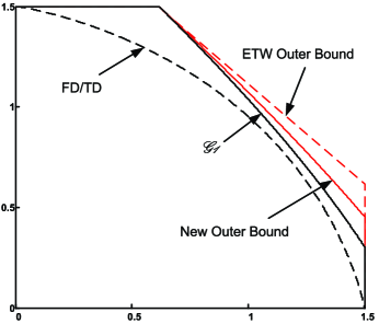
Figure 14: Comparison between different bounds for the mixed Gaussian IC when $1+P_{2}\leq b+abP_{2}$ (Case I) for $P_{1}=7$, $P_{2}=7$, $a=0.6$, and $b=2$.

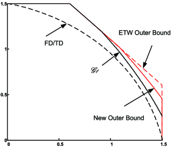
Figure 15: Comparison between different bounds for the mixed Gaussian IC when $1+P_{2}>b+abP_{2}$ and $1-a\leq abP_{1}$ (Case II) for $P_{1}=7$, $P_{2}=7$, $a=0.4$, and $b=1.5$.

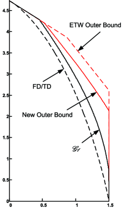
Figure 16: Comparison between different bounds for the mixed Gaussian IC when $1+P_{2}>b+abP_{2}$ and $1-a>abP_{1}$ (Case III) for $P_{1}=7$, $P_{2}=700$, $a=0.01$, and $b=1.5$.

Remark 5

Region $E_{3}$ in Case II and Case III represents a facet that belongs to the capacity region of the mixed Gaussian IC. It is important to note that, surprisingly, this facet is obtainable when the second transmitter uses both the common message and the private message.

Different bounds are compared for the mixed Gaussian IC for Cases I, II, and III in Figures 14, 15, and 16, respectively.

VII Conclusion

We have studied the capacity region of the two-user Gaussian IC. The sum capacities, inner bounds, and outer bounds have been considered for three classes of channels: weak, one-sided, and mixed Gaussian IC. We have used admissible channels as the main tool for deriving outer bounds on the capacity regions.

For the weak Gaussian IC, we have derived the sum capacity for a certain range of channel parameters. In this range, the sum capacity is attained when Gaussian codebooks are used and interference is treated as noise. Moreover, we have derived a new outer bound on the capacity region. This outer bound is tighter than the Kramer’s bound and the ETW’s bound. Regarding inner bounds, we have reduced the computational complexity of the HK achievable region. In fact, we have shown that when Gaussian codebooks are used, the full HK achievable region can be obtained by using the naive HK achievable scheme over three frequency bands.

For the one-sided Gaussian IC, we have presented an alternative proof for the Sato’s outer bound. We have also derived the full HK achievable region when Gaussian codebooks are used.

For the mixed Gaussian IC, we have derived the sum capacity for the entire range of its parameters. Moreover, we have presented a new outer bound on the capacity region that outperforms ETW’s bound. We have proved that the full HK achievable region using Gaussian codebooks is equivalent to that of the one-sided Gaussian IC for a particular range of channel gains. We have also derived a facet that belongs to the capacity region for a certain range of parameters. Surprisingly, this facet is obtainable when one of the transmitters uses both the common message and the private message.

References

- [1] C. E. Shannon, “Two-way communication channels,” in Proc. 4th Berkeley Symp. on Mathematical Statistics and Probability, vol. 1, 1961, pp. 611–644.
- [2] A. B. Carleial, “A case where interference does not reduce capacity,” IEEE Trans. Inform. Theory, vol. IT-21, pp. 569–570, Sept. 1975.
- [3] H. Sato, “The capacity of the gaussian interference channel under strong interference,” IEEE Trans. Inform. Theory, vol. IT-27, pp. 786–788, Nov. 1981.
- [4] R. Ahlswede, “Multi-way communnication channels,” in Proc. 2nd International Symp. on Information theory, U. Tsahkadsor, Armenia, Ed., Sep 2-8 1971, pp. 23–52.
- [5] I. Csiszár and J. Körner, Information Theory: Theorems for Discrete Memoryless Systems. Budapest, Hungary: Hungarian Acad. Sci., 1981.
- [6] R. S. Cheng and S. Verdú, “On limiting characterizations of memoryless multiuser capacity regions,” IEEE Trans. Inform. Theory, vol. 39, pp. 609–612, Mar. 1993.
- [7] T. Cover and J. Thomas, Elements of information theory. NY, John Wiley, 1991.
- [8] T. S. Han and K. Kobayashi, “A new achievable rate region for the interference channel,” IEEE Trans. Inform. Theory, vol. IT-27, pp. 49–6o, Jan. 1981.
- [9] H. Chong, M. Motani, H. Garg, and H. E. Gamal, “On the Han-Kobayashi region for the interference channel,” Submitted to the IEEE Trans. on Inf., Aug. 2006.
- [10] H. Sato, “On degraded gaussian two-user channels,” IEEE Trans. Inform. Theory, vol. IT-24, pp. 637–640, Sept. 1978.
- [11] M. H. M. Costa, “On the Gaussian interference channel,” IEEE Trans. Inform. Theory, vol. IT-31, pp. 607–615, Sept. 1985.
- [12] G. Kramer, “Outer bounds on the capacity of gaussian interference channels,” IEEE Trans. Inform. Theory, vol. 50, pp. 581–586, Mar. 2004.
- [13] R. Etkin, D. Tse, and H. Wang, “Gaussian interference channel capacity to within one bit.” submitted to the IEEE Transactions on Information Theory. Available at http://www.eecs.berkeley.edu/ dtse/pub.html, Feb. 2007.
- [14] T. Liu and P. Viswanath, “An extremal inequality motivated by multi terminal information theoretic problems,” in 2006 Internatinal Symposiun on Information Theory (ISIT), Seattle, WA, July 2006, pp. 1016–1020.
- [15] A. B. Carleial, “Interference channels,” IEEE Trans. Inform. Theory, vol. IT-24, pp. 60–70, Jan. 1978.
- [16] I. Sason, “On achievable rate regions for the gaussian interference channel,” IEEE Trans. Inform. Theory, vol. 50, pp. 1345–1356, June 2004.
- [17] S. Boyd and L. Vandenberghe, Convex Optimization. Cambridge, U.K.: Cambridge Univ. Press, 2003.
- [18] T. Han, “The capacity region of general multiple-access channel with certain correlated sources,” Inform. Contr., vol. 40, no. 1, pp. 37–60, 1979.
- [19] R. T. Rockafellar and R. J.-B. Wets, Variational Analysis. Springer-Verlag, Berlin Heidelberg., 1998.
- [20] R. Etkin, A. Parekh, and D. Tse, “Spectrum sharing for unlicensed bands,” IEEE Journal of Selected Area of Comm., vol. 52, pp. 1813–1827, April 2007.
- [21] S. N. Diggavi and T. Cover, “The worst additive noise under a covariance constraint.” IEEE Trans. Inform. Theory, vol. 47, no. 7, pp. 3072–3081, Nov. 2001.
- [22] S. Ihara, “On the capacity of channels with additive non-Gaussian noise.” Info. Ctrl., vol. 37, no. 1, pp. 34–39, Apr. 1978.
- [23] H. Sato, “An outer bound to the capacity region of broadcast channels,” IEEE Trans. Inform. Theory, vol. IT-24, pp. 374–377, May 1978.
- [24] A. S. Motahari and A. K. Khandani, “Capacity bounds for the gaussian interference channel,” Library Archives Canada Technical Report UW-ECE 2007-26 (Available at http://www.cst.uwaterloo.ca/ pub_tech_rep.html), Aug. 2007.
- [25] X. Shang, G. Kramer, and B. Chen, “A new outer bound and the noisy-interference sum-rate capacity for gaussian interference channels (availabe at: http://arxiv.org/abs/0712.1987),” Submitted to IEEE Trans. Inform. Theory, Dec. 2007.
- [26] V. S. Annapureddy and V. V. Veeravalli, “Sum capacity of the gaussian interference channel in the low interference regime (availabe at: http://arxiv.org/abs/0801.0452),” Proceedings of ITA Workshop, San Diego, CA, Jan. 2008.