Gene regulation in continuous cultures: A unified theory for bacteria and yeasts

Abstract

During batch growth on mixtures of two growth-limiting substrates, microbes consume the substrates either sequentially or simultaneously. These growth patterns are manifested in all types of bacteria and yeasts. The ubiquity of these growth patterns suggests that they are driven by a universal mechanism common to all microbial species. In previous work, we showed that a minimal model accounting only for enzyme induction and dilution explains the phenotypes observed in batch cultures of various wild-type and mutant/recombinant cells. Here, we examine the extension of the minimal model to continuous cultures. We show that: (1) Several enzymatic trends, usually attributed to specific regulatory mechanisms such as catabolite repression, are completely accounted for by dilution. (2) The bifurcation diagram of the minimal model for continuous cultures, which classifies the substrate consumption pattern at any given dilution rate and feed concentrations, provides a a precise explanation for the empirically observed correlation between the growth patterns in batch and continuous cultures. (3) Numerical simulations of the model are in excellent agreement with the data. The model captures the variation of the steady state substrate concentrations, cell densities, and enzyme levels during the single- and mixed-substrate growth of bacteria and yeasts at various dilution rates and feed concentrations. (4) This variation is well approximated by simple analytical expressions that furnish physical insights into the steady states of continuous cultures. Since the minimal model describes the behavior of the cells in the absence of any regulatory mechanisms, it provides a framework for rigorously quantitating the effect of these mechanisms. We illustrate this by analyzing several data sets from the literature.

1 Introduction

The mechanisms of gene regulation are of fundamental importance in biology. They play a crucial role in development by determining the fate of isogenic embroyonic cells, and there is growing belief that the diversity of biological organisms reflects the variation of their regulatory mechanisms (Carroll et al., 2005; Ptashne and Gann, 2002).

Many of the key principles of gene regulation, such as positive, negative, and allosteric control, were discovered by studying the growth of bacteria and yeasts in batch cultures containing one or more growth-limiting substrates. A model system that played a particularly important role is the growth of Escherichia coli on lactose and a mixture of lactose and glucose (Müller-Hill, 1996).

It turns out that the enzymes catalyzing the transport and peripheral catabolism of lactose, such as lactose permease and $\beta$-galactosidase, are synthesized or induced only if lactose is present in the environment. The molecular mechanism of induction was discovered by Monod and coworkers (Jacob and Monod, 1961). They showed that the genes encoding the peripheral enzymes for lactose are contiguous and transcribed sequentially, an arrangement referred to as the lac operon. In the absence of lactose, the lac operon is not transcribed because the lac repressor is bound to a specific site on the lac operon called the operator. This prevents RNA polymerase from attaching to the operon and initiating transcription. In the presence of lactose, transcription of lac is triggered because allolactose, a product of $\beta$-galactosidase, binds to the repressor, and renders it incapable of binding to the operator.

When Escherichia coli is grown on a mixture of glucose and lactose, lac transcription, and hence, the consumption of lactose, is somehow suppressed until glucose is exhausted. During this period of preferential growth on glucose, the peripheral enzymes for lactose are diluted to very small levels. The consumption of lactose begins upon exhaustion of glucose, but only after a certain lag during which the lactose enzymes are built up to sufficiently high levels. Thus, the cells exhibit two exponential growth phases separated by an intermediate lag. Monod referred to this phenomenon as diauxic or “double” growth (Monod, 1942).

Two major molecular mechanisms have been proposed to explain the repression of lac transcription in the presence of glucose:

1. Inducer exclusion (Postma et al., 1993): In the presence of glucose, enzyme IIA^glc, a peripheral enzyme for glucose, is dephosphorylated. The dephosphorylated IIA^glc inhibits lactose uptake by binding to lactose permease. This reduces the intracellular concentration of allolactose, and hence, the transcription rate of the lac operon.
   Genetic evidence suggests that phosphorylated IIA^glc activates adenylate cyclase, which catalyzes the synthesis of cyclic AMP (cAMP). Since glucose uptake results in dephosphorylation of IIA^glc, one expects the cAMP level to decrease in the presence of glucose. This forms the basis of the second mechanism of lac repression.

2. cAMP activation (Ptashne and Gann, 2002): It has been observed that the recruitment of RNA polymerase to promoter is inefficient unless a protein called catabolite activator protein (CAP) is bound to a specific CAP site on the promoter. Furthermore, CAP has a low affinity for the CAP site, but when bound to cAMP, its affinity increases dramatically. The inhibition of lac transcription by glucose is then explained as follows.
   In the presence of lactose alone (i.e., no glucose), the cAMP level is high. Hence, CAP becomes cAMP-bound, attaches to the CAP site, and promotes transcription by recruiting RNA polymerase. When glucose is added to the culture, the cAMP level decreases by the mechanism described above. Consequently, CAP, being cAMP-free, fails to bind to the CAP site, and lac transcription is abolished.

Mechanistic mathematical models of the glucose-lactose diauxie appeal to both these mechanisms (Kremling et al., 2001; Santillán et al., 2007; Dedem and Moo-Young, 1975; Wong et al., 1997)

Over the last few decades, microbial physiologists have accumulated a vast amount of data showing that diauxic growth is ubiquitous (reviewed in Egli, 1995; Harder and Dijkhuizen, 1982; Kovarova-Kovar and Egli, 1998). It occurs in diverse microbial species and numerous pairs of substitutable substrates (satisfying identical nutrient requirements). In many of these systems, the above mechanisms play no role. For instance, cAMP is not detectable in gram-positive bacteria (Mach et al., 1984), and has little effect on the transcription of peripheral enzymes in pseudomonads (Collier et al., 1996) and yeasts (Eraso and Gancedo, 1984). It has been proposed that in these cases, the mechanisms of repression are analogous to those of the lac operon, but involve different transcription factors, such as CcpA in gram-positive bacteria (Chauvaux, 1996), Crc in pseudomonads (Morales et al., 2004), and MigA in yeasts (Johnston, 1999).

Paradoxically, there is growing evidence that cAMP activation and inducer exclusion are not sufficient for explaining lac repression. Not long after the discovery of cAMP activation (Perlman and Pastan, 1968; Ullmann and Monod, 1968), Ullmann presented several lines of evidence showing that this mechanism played a relatively modest role in diauxic growth (Ullmann, 1974). But the most compelling evidence was obtained by Aiba and coworkers, who showed that the cAMP levels are essentially the same during the first and second growth phases; furthermore, glucose-mediated lac repression persists in the presence of high (5mM) exogenous cAMP levels, and in mutants of E. coli in which the ability of cAMP to influence lac transcription is completely abolished (Inada et al., 1996; Kimata et al., 1997). In Section 3.1, we shall show that the positive correlation between lac expression and intracellular cAMP levels (Epstein et al., 1975), which forms the foundation of the cAMP activation mechanism, does not reflect a causal relationship: The observed variation of lac expression is almost entirely due to dilution (rather than cAMP activation).

The persistence of lac repression in cAMP-independent cells has led to the hypothesis that inducer exclusion is the sole cause of repression (Kimata et al., 1997). However, this mechanism exerts a relatively mild effect. The lactose uptake rate is inhibited only $\sim$50% in the presence of glucose (McGinnis and Paigen, 1969).

Thus, transcriptional repression, by itself, cannot explain the several hundred-fold repression of lac during the first exponential growth phase of diauxic growth. In earlier work, we have shown that complete repression is predicted by a minimal model accounting for only induction and growth (Narang, 1998a, 2006).

Yet another phenomenon that warrants an explanation is the empirically observed correlation between the substrate consumption pattern and the specific growth on the individual substrates. For instance, in the case of diauxic growth, it has been observed that:

In most cases, although not invariably, the presence of a substrate permitting a higher growth rate prevents the utilization of a second, ‘poorer’ substrate in batch culture (Harder and Dijkhuizen, 1982).

It turns out that sequential consumption of substrates is not the sole growth pattern in batch cultures. Monod observed that in several cases of mixed-substrate growth, there was no diauxic lag (Monod, 1942, 1947), and subsequent studies have shown that both substrates are often consumed simultaneously (Egli, 1995). The occurrence of simultaneous substrate consumption also appears to correlate with the specific growth rates on the individual substrates. Based on a comprehensive review of the literature, Egli notes that:

Especially combinations of substrates that support medium or low maximum specific growth rates are utilized simultaneously (Egli, 1995).

Recently, we have shown that the minimal model provides a natural explanation for the foregoing correlations, which hinges upon the fact that the enzyme dilution rate is proportional to the specific growth rate (Narang and Pilyugin, 2007a). Roughly, substrates that support high growth rates lead to such high enzyme dilution rates that the enzymes of the “less preferred” substrates are diluted to near-zero levels. On the other hand, substrates that support low growth rates fail to efficiently dilute the enzymes of the other substrates. A more precise statement of this argument is given in Section 3.3.

Now, all the experimental results described above were obtained in batch cultures. However, since the invention of the chemostat, microbial physiologists have acquired extensive data on microbial growth in continuous cultures. Detailed analyses of this data have revealed well-defined patterns or motifs that occur in diverse microbial species growing on various substrates (Egli, 1995; Harder and Dijkhuizen, 1982; Kovarova-Kovar and Egli, 1998). The goal of this work is to show that the minimal model also accounts for the patterns observed in continuous cultures. We begin by giving a brief preview of these patterns in single- and mixed-substrate cultures.

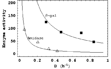
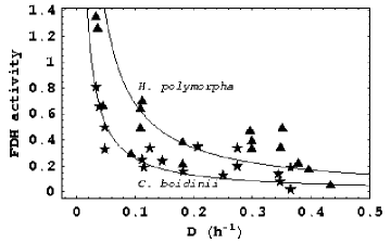
Figure 1: If the induction rate of the peripheral enzyme is independent of the inducer level, its activity decreases with the dilution rate. (a) The activities of $\beta$-galactosidase (Silver and Mateles, 1969, Fig. 1) and amidase (Clarke et al., 1968, Fig. 2) during growth of the constitutive mutants, E. coli B6b2 and P. aeruginosa C11, on lactose and acetamide, respectively. (b) The activity of formaldehyde dehydrogenase (FDH) during glucose-limited growth of H. polymorpha and C. boidinii (Egli et al., 1980, Fig. 1c,d). The curves in (a) and (b) shows the fits to eqs. (17) and (18), respectively.

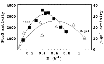
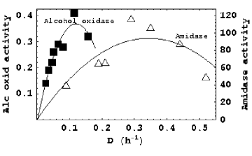
Figure 2: The activity of inducible enzymes passes through a maximum at an intermediate dilution rate. (a) Activities of PtsG (Seeto et al., 2004, Fig. 1) and $\beta$-galactosidase (Silver and Mateles, 1969, Fig. 4a) during glucose-limited growth of E. coli K12 and lactose-limited growth of E. coli B6, respectively. (b) Activities of alcohol oxidase (Egli and Harder, 1983, Fig. 1) and amidase (Clarke et al., 1968, Fig. 1) during methanol-limited growth of H. polymorpha and acetamide-limited growth of P. aeroginosa, respectively.

In chemostats limited by a single substrate, steady growth can be maintained at all dilution rates up to the critical dilution rate at which the cells wash out. At subcritical dilution rates, the peripheral enzyme activities of various cell types and growth-limiting substrates invariably show one of the following two trends (Harder and Dijkhuizen, 1982):

1. If the peripheral enzyme is fully constitutive, its activity decreases monotonically with the dilution rate (Fig. 1a). The very same trend is observed even if the peripheral enzyme is inducible, but the nutrient medium lacks substrates that can induce the synthesis of the enzyme (Fig. 1b and Fig. 6d).

2. If the peripheral enzyme is inducible and the medium contains the inducing substrate, the enzyme activity passes through a maximum at an intermediate dilution rate (Fig. 2).

Clarke and coworkers were the first to observe these trends during acetamide-limited growth of wild-type and constitutive mutants of P. aeruginosa (Clarke et al., 1968). They hypothesized that in wild-type cells, the amidase activity exhibits a maximum (Fig. 2b) due to the balance between induction and catabolite repression. Specifically,

at low dilution rates, catabolite repression is minimal and the rate of amidase synthesis is dependent mainly on the rate at which acetamide is presented to the bacteria. Thus, with increase in dilution rate the amidase specific activity under steady state conditions increases. However, above $D=0.30$ h^-1 the growth rate has increased to the point where metabolic intermediates are being formed at a sufficiently high rate to cause significant catabolite repression. At higher dilution rates catabolite repression becomes dominant and at $D=0.6$ h^-1 the enzyme concentration has decreased considerably (Clarke et al., 1968, p. 232).

In constitutive mutants, the enzyme activity decreases monotonically (Fig. 1a) because “they lack completely the part where, in the curves for the wild-type strain, … induction is dominant.” These hypotheses have subsequently been invoked to rationalize the similar trends found in the wild-type cells and constitutive mutants of many other microbial systems (reviewed in Dean, 1972; Matin, 1978; Toda, 1981). We shall show below that the decline of the enzyme activity (at all $D$ in constitutive mutants, and at high $D$ in wild-type cells) is entirely due to dilution, rather than catabolite repression.

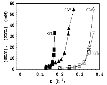
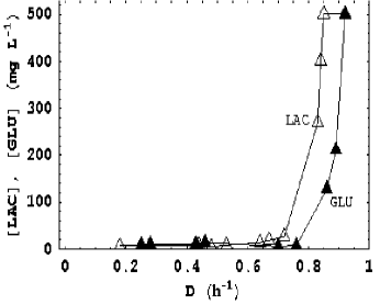
Figure 3: Simultaneous and preferential growth patterns in continuous cultures. (a) During growth of H. polymorpha on a mixture of xylose and glycerol, both substrates are consumed at all dilution rates up to washout (calculated from Fig. 3 of Brinkmann and Babel, 1992). Closed and open symbols show the substrate concentrations during single- and mixed-substrate growth, respectively. (b) During growth of E. coli B on a mixture of glucose and lactose, consumption of lactose ceases at a dilution rate below the (washout) dilution rate at which consumption of glucose ceases (Silver and Mateles, 1969, Fig. 3).

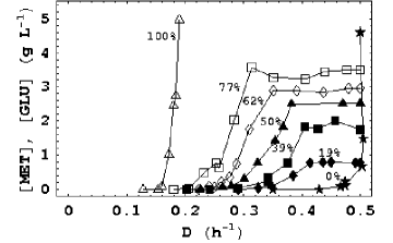
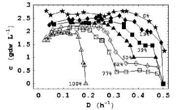
Figure 4: Variation of the substrate concentrations and cell density during mixed-substrate growth of H. polymorpha on a mixture of glucose and methanol (Egli et al., 1986, Fig. 2). The total feed concentration of glucose and methanol was 5 g L^-1 in all the experiments. The percentages show the mass percent of methanol in the feed. The critical dilution rates on pure methanol (curve labeled 100%) and pure glucose (curve labeled 0%) are $\sim$0.2 and $\sim$0.5 h^-1, respectively.

In chemostats limited by pairs of carbon sources, two types of steady state profiles have been observed. Importantly, these profiles correlate with, and in fact, can be predicted by, the substrate consumption pattern observed in substrate-excess batch cultures. Indeed, pairs of substrates consumed simultaneously in substrate-excess batch cultures are consumed simultaneously in continuous cultures at all dilution rates up to washout (Fig. 3a). In contrast, pairs of substrates that show diauxic growth in substrate-excess batch cultures are consumed simultaneously in continuous cultures only if the dilution rate is sufficiently small. For instance, during growth of Escherichia coli B on a mixture of glucose and lactose, consumption of the “less preferred” substrate, lactose, declines sharply at an intermediate dilution rate, beyond which only glucose is consumed (Fig. 3b). This growth pattern has been observed in several other systems (reviewed in Harder and Dijkhuizen, 1976, 1982), but the most comprehensive data was obtained in studies of the methylotrophic yeasts, Hansenula polymorpha and Candida boidinii, with mixtures of methanol + glucose (Egli et al., 1980, 1982b, 1982a, 1986). These studies, which were performed with various feed concentrations of glucose and methanol, revealed several well-defined patterns:

1. The sharp decline in methanol consumption at an intermediate dilution rate is analogous to the phenomenon of diauxic growth in batch cultures inasmuch as it is triggered by a precipitous drop in the activities of the peripheral enzymes for methanol, the “less preferred” substrate. The transition dilution rate was empirically defined by Egli as the dilution rate at which the concentration of the “less preferred substrate” achieves a sufficiently high value, e.g., half of the feed concentration (Egli et al., 1986, Fig. 1).

2. The transition dilution rate is always higher than the critical dilution rate on methanol (Fig. 4a). This was referred to as the enhanced growth rate effect, since methanol was consumed at dilution rates significantly higher than the critical dilution rate in cultures fed with pure methanol.

3. The transition dilution rate varies with the feed composition — the larger the fraction of methanol in the feed, the smaller the transition dilution rate (Fig. 4a).

These and several other general trends, discussed later in this work, have been observed in a wide variety of bacteria and yeasts (reviewed in Egli, 1995; Kovarova-Kovar and Egli, 1998).

The occurrence of the very same growth patterns in such diverse organisms suggests that they are driven by a universal mechanism common to all species. Thus, we are led to consider the minimal model, which accounts for only those processes — induction and growth — that occur in all microbes. In earlier work, computational studies of a variant of the minimal model showed that it captures all the growth patterns discussed above (Narang, 1998b). Here, we perform a rigorous bifurcation analysis of the model to obtain a complete classification of the growth patterns at any given dilution rate and feed concentrations. The analysis reveals new features, such as threshold effects, that were missed in our earlier work. It also provides simple explanations for the following questions:

1. During single-substrate growth of wild-type cells, why does the activity of the peripheral enzymes pass through a maximum?

2. During growth on mixtures of substrates, what are conditions under which (a) both substrates are consumed at all dilution rates up to washout (Fig. 3a), and (b) consumption of one of the substrates ceases at an intermediate dilution rate (Fig. 3b)?

3. Why does the transition dilution rate exist? Why is it always larger than the critical dilution rate of the “less preferred” substrate, and why does it vary with the feed concentrations (Fig. 4a)?

Finally, we show that under the conditions typically used in experiments, the physiological (intracellular) steady states are completely determined by only two parameters, namely, the dilution rate and the mass fraction of the substrates in the feed (rather than the feed concentrations per se). In fact, we derive explicit expressions for the steady state substrate concentrations, cell density, and enzyme levels, which provide physical insight into the variation of these quantities with the dilution rate and feed concentrations.

2 Theory

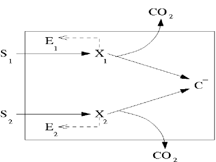
Figure 5: Kinetic scheme of the minimal model (Narang, 1998a).

Fig. 5 shows the kinetic scheme of the minimal model. Here, $S_{i}$ denotes the $i^{{\rm th}}$ exogenous substrate, $E_{i}$ denotes the “lumped” peripheral enzymes for $S_{i}$, $X_{i}$ denotes internalized $S_{i}$, and $C^{-}$ denotes all intracellular components except $E_{i}$ and $X_{i}$ (thus, it includes precursors, free amino acids, and macromolecules).

We assume that:

1. The concentrations of the intracellular components, denoted $e_{i}$, $x_{i}$, and $c^{-}$, are based on the dry weight of the cells (g per g dry weight of cells, i.e., g gdw^-1). The concentrations of the exogenous substrate and cells, denoted $s_{i}$ and $c$, are based on the volume of the reactor (g L^-1 and gdw L^-1, respectively). The rates of all the processes are based on the dry weight of the cells (g gdw^-1 h^-1). We shall use the term specific rate to emphasize this point.
   The choice of these units implies that if the concentration of any intracellular component, $Z$, is $z$ g gdw^-1, then the evolution of $z$ in a continuous culture operating at dilution rate, $D$, is given by

   $$\frac{dz}{dt}=r_{z}^{+}-r_{z}^{-}-\left(D+\frac{1}{c}\frac{dc}{dt}\right)z,$$

   where $r_{z}^{+}$ and $r_{z}^{-}$ denote the specific rates of synthesis and degradation of $Z$, and $Dz$ is the specific rate of efflux of $Z$ from the chemostat. It is shown below that the sum, $Dz+(1/c)(dc/dt)z$, is precisely the rate of dilution of $Z$ due to growth.

2. The transport and peripheral catabolism of $S_{i}$ is catalyzed by a unique system of peripheral enzymes, $E_{i}$. The specific uptake rate of $S_{i}$, denoted $r_{s,i}$, follows the modified Michaelis-Menten kinetics

   $$r_{s,i}\equiv V_{s,i}e_{i}\frac{s_{i}}{K_{s,i}+s_{i}},$$

   where $V_{s,i}$ is a fixed constant, i.e., inducer exclusion is negligible.

3. Part of the internalized substrate, denoted $X_{i}$, is converted to $C^{-}$. The remainder is oxidized to ${\rm CO_{2}}$ in order to generate energy.

   1. The conversion of $X_{i}$ to $C^{-}$ and ${\rm CO_{2}}$ follows first-order kinetics, i.e.,

      $$r_{x,i}\equiv k_{x,i}x_{i}.$$

   2. The fraction of $X_{i}$ converted to $C^{-}$, denoted $Y_{i}$, is constant. It is shown below that $Y_{i}$ is essentially identical to the yield of biomass on $S_{i}$. This assumption is therefore tantamount to assuming that the yield of biomass on a substrate is unaffected by the presence of another substrate in the medium.

4. The internalized substrate also induces the synthesis of $E_{i}$, which is assumed to controlled entirely by the initiation of transcription (i.e., mechanisms such as attenuation and proteolysis are neglected).

   1. The specific synthesis rate of $E_{i}$ follows the hyperbolic Yagil & Yagil kinetics (Yagil and Yagil, 1971),

      $$r_{e,i}^{+}\equiv V_{e,i}\frac{1+x_{i}}{1+\alpha_{i}+x_{i}},$$ (1)

      where $V_{e,i}$ is a fixed constant, i.e., catabolite repression is negligible. In the particular case of negatively controlled operons (modulated by repressors), $V_{e,i}$ and $\alpha_{i}$ can be expressed in terms of parameters associated with kinetics of RNAP-promoter and repressor-operator binding, respectively. In other cases, (1) must be viewed as a phenomenological description of the induction kinetics.

   2. Enzyme degradation is a first-order process, i.e., the specific rate of enzyme degradation is

      $$r_{e,i}^{-}=k_{e,i}e_{i}.$$

   3. The enzymes are synthesized at the expense of $C^{-}$, and their degradation produces $C^{-}$.

Given these assumptions, the mass balances yield the equations

$$\frac{ds_{i}}{dt} =D\left(s_{f,i}-s_{i}\right)-r_{s,i}c,$$ (2)

$$\frac{dx_{i}}{dt} =r_{s,i}-r_{x,i}-\left(D+\frac{1}{c}\frac{dc}{dt}\right)x_{i},$$ (3)

$$\frac{de_{i}}{dt} =r_{e,i}^{+}-r_{e,i}^{-}-\left(D+\frac{1}{c}\frac{dc}{dt}\right)e_{i},$$ (4)

$$\frac{dc^{-}}{dt} =\left(Y_{1}r_{x,1}+Y_{2}r_{x,2}\right)-\left(r_{e,1}^{+}-r_{e,1}^{-}\right)-\left(r_{e,2}^{+}-r_{e,2}^{-}\right)-\left(D+\frac{1}{c}\frac{dc}{dt}\right)c^{-},$$ (5)

where $s_{f,i}$ denotes the concentration of $S_{i}$ in the feed to the chemostat.

Following Fredrickson, we observe that eqs. (3)–(5) implicitly define the specific growth rate and the evolution of the cell density (Fredrickson, 1976). Indeed, since $x_{1}+x_{2}+e_{1}+e_{2}+c^{-}=1$, addition of (3)–(5) yields

$$0=r_{g}-\left(D+\frac{1}{c}\frac{dc}{dt}\right)\Leftrightarrow\frac{dc}{dt}=\left(r_{g}-D\right)c,$$ (6)

where

$$r_{g}\equiv\sum_{i=1}^{2}r_{s,i}-\sum_{i=1}^{2}(1-Y_{i})r_{x,i}$$ (7)

is the specific growth rate. As expected, it is the net rate of substrate accumulation in the cells. It follows from (6) that the last term in eqs. (3)–(5) is precisely the dilution rate of the corresponding physiological (intracellular) variables.

The equations can be simplified further because $k_{x,i}^{-1}$, the turnover time for $X_{i}$, is small (on the order of seconds to minutes). Thus, $x_{i}$ rapidly attains quasisteady state, resulting in the equations

$$\frac{ds_{i}}{dt} =D\left(s_{f,i}-s_{i}\right)-r_{s,i}c,$$ (8)

$$\frac{de_{i}}{dt} =r_{e,i}^{+}-\left(r_{g}+k_{e,i}\right)e_{i},$$ (9)

$$\frac{dc}{dt} =\left(r_{g}-D\right)c,$$ (10)

$$x_{i} \approx\frac{V_{s,i}e_{i}s_{i}/\left(K_{s,i}+s_{i}\right)}{k_{x,i}},$$ (11)

$$r_{g} \approx Y_{1}r_{s,1}+Y_{2}r_{s,2},$$ (12)

where (11)–(12) follow from the quasisteady state relation, $0\approx r_{s,i}-r_{x,i}$.

It is worth noting that:

1. The parameter, $Y_{i}$, which was defined as the fraction of $X_{i}$ converted to $C^{-}$, is essentially the yield of biomass on $S_{i}$. Indeed, substituting the relation, $r_{x,i}\approx r_{s,i}$ in (7) shows that after quasisteady state has been attained, $Y_{i}$ approximates the fraction of $S_{i}$ that accumulates in the cell.

2. Although we have assumed that $Y_{i}$ is constant, the validity of (12) does not rest upon this assumption. It is true even if the yields are variable (i.e., depend on the physiological state).

3. Enzyme induction is subject to positive feedback. This becomes evident if (11) is substituted in (1): The quasisteady state induction rate, $r_{e,i}^{+}$, is an increasing function of $e_{i}$. The positive feedback reflects the cyclic structure of enzyme synthesis that is inherent in Fig. 5: $E_{i}$ promotes the synthesis of $X_{i}$, which, in turn, stimulates the induction of $E_{i}$.

We shall appeal to these facts later.

The equations for batch growth are obtained from the above equations by letting $D=0$. In what follows, we shall be particularly concerned with the initial evolution of the enzymes in experiments performed with sufficiently small inocula. Under this condition, the substrate consumption for the first few hours is so small that the substrate concentrations remain essentially constant at their initial levels, $s_{0,i}$. In the face of this quasiconstant environment, the enzyme activities move toward a quasisteady state corresponding to exponential (balanced) growth. This motion is given by the equations

$$\frac{de_{i}}{dt} =r_{e,i}^{+}-\left(r_{g}+k_{e,i}\right)e_{i},$$ (13)

$$x_{i} \approx\frac{V_{s,i}e_{i}s_{0,i}/\left(K_{s,i}+s_{0,i}\right)}{k_{x,i}},$$ (14)

$$r_{g} \approx Y_{1}V_{s,1}e_{1}\frac{s_{0,1}}{K_{s,1}+s_{0,1}}+Y_{2}V_{s,2}e_{2}\frac{s_{0,2}}{K_{s,2}+s_{0,2}},$$ (15)

obtained by letting $s_{i}\approx s_{0,i}$ in eqs. (11)–(12). The steady state(s) of these equations represent the quasisteady state enzyme activities attained during the first exponential growth phase.

We note finally that the cells sense their environment through the ratio,

$$\sigma_{i}\equiv\frac{s_{i}}{K_{s,i}+s_{i}},$$

which characterizes the extent to which the permease is saturated with $S_{i}$. Not surprisingly, we shall find later on that the physiological steady states depend on the ratio, $\sigma_{i}$, rather than the substrate concentrations per se. It is, therefore, convenient to define the ratios

$$\sigma_{0,i}\equiv\frac{s_{0,i}}{K_{s,i}+s_{0,i}},\;\sigma_{f,i}\equiv\frac{s_{f,i}}{K_{s,i}+s_{f,i}}.$$

For a given cell type, $\sigma_{i}$, $\sigma_{0,i}$, $\sigma_{f,i}$ are increasing functions of $s_{i}$, $s_{i,0}$, $s_{f,i}$, respectively, and can be treated as surrogates for the corresponding substrate concentrations. In what follows, we shall frequently refer to $\sigma_{i}$, $\sigma_{0,i}$, and $\sigma_{f,i}$ as the substrate concentration, initial substrate concentration, and feed concentration, respectively.

3 Results

3.1 The role of regulation

Before analyzing the foregoing equations for batch and continuous cultures, we pause to consider the role of regulatory mechanisms. This is important because the literature places great emphasis on the regulatory mechanisms, whereas the model neglects them completely ($V_{s,i}$ and $V_{e,i}$ are assumed to be constants). It is therefore relevant to ask: To what extent do the regulatory mechanisms control gene expression? To address this question, we shall focus on the well-characterized lac operon in E. coli. The analysis shows that cAMP activation and inducer exclusion cannot explain the strong repression observed in experiments.

3.1.1 cAMP activation

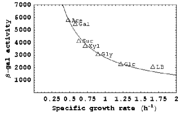
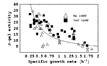
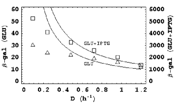
Figure 6: The relative roles of dilution and cAMP activation in lac induction. (a) Variation of the $\beta$-galactosidase activity with intracellular cAMP level during exponential growth of the lac-constitutive strain E. coli X2950 on various carbon sources (Epstein et al., 1975, Fig. 2). (b,c) During batch growth of (b) E. coli MC4100 $\lambda$CPT100 (Kuo et al., 2003, Fig. 2) and (c) E. coli NC3 (Wanner et al., 1978, Fig. 1) on various carbon sources, the steady state $\beta$-galactosidase activity is inversely proportional to the specific growth rate on the carbon source. Moreover, the $\beta$-galactosidase activity increases at most 2-fold if 5mM cAMP is added to the medium ($\blacksquare$). (d) The inverse relationship is satisfied at $D\gtrsim 0.4$ h^-1 in continuous cultures of E. coli K12 W3110 grown on glucose and glucose + 1mM IPTG (Kuo et al., 2003, Fig. 1). The curves in (b)–(c) and (d) show the fits to (16) and (17), respectively.

Interest in cAMP as a lac regulator began when it was discovered that the lac induction rate increased $\sim$2-fold upon addition of cAMP to glucose-limited cultures (Perlman and Pastan, 1968; Ullmann and Monod, 1968). However, this remained a hypothesis until Epstein et al showed that the lac induction rate increased with the intracellular cAMP levels (Fig. 6a). They obtained this relationship by measuring the $\beta$-galactosidase activities and intracellular cAMP levels during exponential growth of the lac-constitutive strain E. coli X2950 on a wide variety of carbon sources. The use of a constitutive strain served to eliminate inducer exclusion: In such cells, the repressor-operator binding is impaired so severely that $\alpha_{i}\approx 0$, and the induction rate is unaffected by the inducer level ($r_{e,i}^{+}\approx V_{e,i}$). The diverse carbon sources provided a way of varying the intracellular cAMP levels: In general, the lower the specific growth rate on a substrate, the higher the intracellular cAMP level (Buettner et al., 1973).

Although Fig. 6a shows a correlation between the cAMP level and the lac induction rate, it does not prove that there is a causal relationship between them. Indeed, since protein degradation is negligible in substrate-excess batch cultures (Mandelstam, 1958), (13) yields

$$e_{i}\approx\frac{r_{e,i}^{+}}{r_{g}}\approx\frac{V_{e,i}}{r_{g}}.$$ (16)

Thus, the steady state enzyme level depends on the ratio of the specific induction and growth rates. Since the substrates that yield high intracellular cAMP levels also support low specific growth rates, it is conceivable that Fig. 6a reflects the variation of the specific growth rate, $r_{g}$, rather than the specific induction rate, $V_{e,i}$.

Eq. (16) provides a simple criterion for checking if the specific induction rate varied in the experiments: Evidently, $V_{e,i}$ varies if and only if $e_{i}$ is not inversely proportional to $r_{g}$. Unfortunately, we cannot check the data in Fig. 6a with this criterion, since the authors did not report the specific growth rates of the carbon sources. However, the very same experiments have been performed by others (Kuo et al., 2003; Wanner et al., 1978), and this data shows that the $\beta$-galactosidase activity is inversely proportional to $r_{g}$ (Figs. 6b,c). It follows that in Figs. 6b and 6c, the $\beta$-galactosidase activity varies almost entirely due to dilution. The influence of cAMP on lac transcription is very modest, a fact that is further confirmed by the very marginal (<2-fold) improvement of the $\beta$-galactosidase activity in the presence of 5mM cAMP (Figs. 6c). The same is likely to be true of the data in Fig. 6a. Thus, the data from Epstein et al., 1975, which is extensively cited to support the existence of cAMP-mediated lac control, forces upon us just the opposite conclusion: cAMP has virtually no effect on the lac induction rate.

The data from continuous cultures also implies the absence of significant cAMP activation. Indeed, (9) implies that when lac-constitutive mutants of E. coli are grown in continuous cultures, the steady state $\beta$-galactosidase activity at sufficiently high dilution rates is given by the relation

$$e_{i}\approx\frac{V_{e,i}}{D}.$$ (17)

This relationship also holds for wild-type cells if the medium contains saturating concentrations of the gratuitous inducer, IPTG. In both cases, cAMP control is significant only if $e_{i}$ is not inversely proportional to $D$. But experiments performed with lac-constitutive mutants (Fig. 1a) and wild-type cells exposed to saturating IPTG levels (Fig. 6d) show that $\beta$-galactosidase activity is inversely proportional to $D$ for sufficiently large $D$.

Catabolite repression also appears to be insignificant in cell types other than E. coli. The amidase activity is inversely proportional to $D$ in the constitutive mutant P. aeroginosa C11 (Fig. 1a). Moreover, this declining trend is not due to catabolite repression, as postulated by Clarke and coworkers — it reflects the effect of dilution. Likewise, the activity of alcohol oxidase is inversely proportional to $D$ when H. polymorpha and C. boidinii are grown in glucose-limited chemostats. In this case, (9) implies that at sufficiently large dilution rates

$$e_{i}=\frac{V_{e,i}}{1+\alpha_{i}}\frac{1}{D},$$ (18)

which is formally similar to (17).

3.1.2 Inducer exclusion

The data shows that inducer exclusion certainly exists. When glucose or glucose-6-phosphate are added to a culture growing exponentially on lactose, the specific uptake rate of lactose declines $\sim$2-fold (McGinnis and Paigen, 1969, Figs. 3,5). Likewise, in the presence of glucose, the intracellular inducer concentration, as measured by the accumulation of radioactively labeled TMG, also decreases $\sim$2-fold (Winkler and Wilson, 1967, Fig. 1). But this modest decrease cannot account for the dramatic repression of the lac operon during diauxic growth: The addition of glucose-6-phosphate to a culture growing on lactose decreases the activity of $\beta$-galactosidase $\sim$300-fold after only 4 generations of growth (Hogema et al., 1998, Table 1).

We conclude that cAMP activation and inducer exclusion do influence the lac induction rate, but their effect is not commensurate with the experimentally observed repression. We show below that the minimal model predicts complete transcriptional repression, despite the absence of any regulatory mechanism.

3.2 Single-substrate growth

In wild-type cells, the repressor-operator binding is so tight that $\alpha_{i}$ is large compared to 1. This is true even in the case of glucose ($\alpha_{i}$=5–10), which is often treated as a substrate consumed by constitutive enzymes (Notley-McRobb and Ferenci, 2000, Table 3). Under these conditions, the basal induction rate is small compared to the fully induced induction rate. Hence, at all but the smallest inducer levels, the specific induction rate can be approximated by the expression

$$V_{e,i}\frac{x_{i}}{K_{e,i}+x_{i}},\;K_{e,i}\equiv\frac{\alpha_{i}}{K_{x,i}},$$ (19)

and the quasisteady state induction rate, obtained by substituting (11) in (19), is

$$V_{e,i}\frac{e_{i}\sigma_{i}}{\bar{K}_{e,i}+e_{i}\sigma_{i}},\;\bar{K}_{e,i}\equiv\frac{K_{e,i}k_{x,i}}{V_{s,i}}.$$

It is useful to make this approximation because the equations become amenable to rigorous analysis and yield simple physical insights. In the rest of the paper, we shall confine our attention to these idealized perfectly inducible systems.

We begin by considering the growth of cultures limited by a single substrate, say, $S_{1}$. Under this condition, $s_{2}=e_{2}=0$, and the steady state values of the remaining variable satisfy the equations

$$0 =\frac{ds_{1}}{dt}=D(s_{f,1}-s_{1})-V_{s,1}e_{1}\sigma_{1}c,$$ (20)

$$0 =\frac{de_{1}}{dt}=V_{e,1}\frac{e_{1}\sigma_{1}}{\bar{K}_{e,1}+e_{1}\sigma_{1}}-\left(Y_{1}V_{s,1}e_{1}\sigma_{1}+k_{e,1}\right)e_{1},$$ (21)

$$0 =\frac{dc}{dt}=\left(Y_{1}V_{s,1}e_{1}\sigma_{1}-D\right)c,$$ (22)

$$x_{1} \approx\frac{V_{s,1}e_{1}\sigma_{1}}{k_{x,1}}.$$ (23)

These equations have three types of steady states: $e_{1}>0$, $e_{2}=0$, $c>0$, denoted $E_{101}$; $e_{1}>0$, $e_{2}=0$, $c=0$, denoted $E_{100}$; and $e_{1}=0$, $e_{2}=0$, $c=0$, denoted $E_{000}$. The first two steady states correspond to the persistence and washout steady states of the classical Monod model (Herbert et al., 1956). The third steady state, $E_{000}$, is a consequence of perfect inducibility — it exists precisely because the specific induction rate is zero in the absence of the inducer.

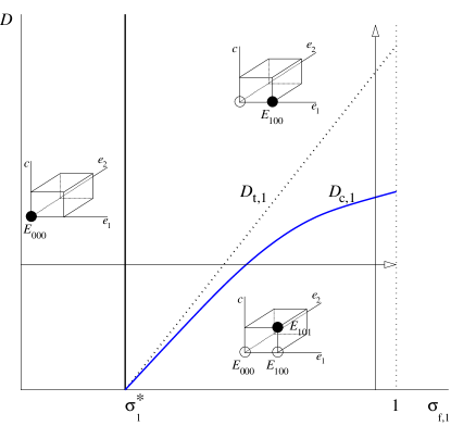
Figure 7: Bifurcation diagram for single-substrate growth on $S_{1}$. The blue curve denotes the curve of the critical dilution rate, $D_{c,1}$, and $\sigma_{1}^{*}$ denotes the threshold feed concentration. The 3-D insets depict the existence and stability of the steady states at any given $\sigma_{f,1}$ and $D$. Stable and unstable steady states are represented by full and open circles, respectively. The dashed line shows the transition dilution rate, $D_{t,1}$, which plays a crucial role in mixed-substrate growth (Section 3.3). The figure is not drawn to scale: Since $k_{e,1}\sim 0.05$ h^-1 and $V_{e,1}/\bar{K}_{e,1}\sim 1$ h^-1, the threshold, $\sigma_{1}^{*}\equiv k_{e,1}/(V_{e,1}/\bar{K}_{e,1})$, is on the order of 0.05.

Fig. 7 shows the bifurcation diagram for eqs. (20)–(23). It can be inferred from the following facts derived in Appendix B.

1. $E_{000}$ always exists, but it is stable if and only if

   $$\frac{V_{e,1}\sigma_{f,1}}{\bar{K}_{e,1}}<k_{e,1}\Leftrightarrow\sigma_{f,1}<\sigma_{1}^{*}\equiv\frac{k_{e,1}}{V_{e,1}/\bar{K}_{e,1}}.$$

   Thus, growth cannot be sustained in a chemostat if the feed concentration is below the threshold level, $\sigma_{1}^{*}$. Under this condition

   $$r_{e,1}^{+}=V_{e,1}\frac{e_{1}\sigma_{1}}{\bar{K}_{e,1}+e_{1}\sigma_{1}}\leq V_{e,1}\frac{e_{1}\sigma_{f,1}}{\bar{K}_{e,1}+e_{1}\sigma_{f,1}}\leq k_{e,1}e_{1},$$

   i.e., the induction rate of $E_{1}$ never exceeds the degradation rate. Hence, as $t\rightarrow\infty$, $e_{1}$ approaches zero, and $c,\sigma_{1}$ tend toward $0,\sigma_{f,1}$, respectively.

2. $E_{100}$ exists if and only if $\sigma_{f,1}>\sigma_{1}^{*}$, in which case it is given by the relations, $c=0$, $\sigma_{1}=\sigma_{f,1}$, and

   $$e_{1}=\frac{-\left(\bar{K}_{e,1}+\frac{k_{e,1}}{Y_{1}V_{s,1}}\right)+\sqrt{\left(\bar{K}_{e,1}+\frac{k_{e,1}}{Y_{1}V_{s,1}}\right)^{2}+\frac{4V_{e,1}}{Y_{1}V_{s,1}}\left(\sigma_{f,1}-\sigma_{1}^{*}\right)}}{2\sigma_{f,1}}.$$

   It is stable if and only if $D$ exceeds the critical dilution rate

   $$D_{c,1}\equiv Y_{1}V_{s,1}e_{1}\sigma_{f,1}.$$ (24)

   Evidently, $D_{c,1}$ is an increasing function of $\sigma_{f,1}$ that is zero when $\sigma_{f,1}=\sigma_{1}^{*}$. We show below that $D_{c,1}$ is the maximum specific growth rate that can be sustained in the chemostat ($r_{g}<D_{c,1})$.
   At first sight, this steady state poses a paradox: There are no cells in the chemostat, and yet, these non-existent cells have positive enzyme levels. The paradox disappears once it is recognized that $E_{100}$ reflects the long-run behavior of a small inoculum introduced into a sterile chemostat operating at $\sigma_{f,1}>\sigma_{1}^{*}$ and $D>D_{c,1}$. As $t\rightarrow\infty$, the specific growth rate of the cells approaches the maximum level, $D_{c,1}$. However, since $r_{g}<D_{c,1}$,

   $$\frac{dc}{dt}=\left(r_{g}-D\right)c<\left(D_{c,1}-D\right)c<0,$$

   so that $c\rightarrow 0$, $\sigma_{1}\rightarrow\sigma_{f,1}$, and $e_{1}$ approaches the positive value given above. Thus, in contrast to $E_{000}$, the cells fail to accumulate despite sustained induction of the enzymes because the dilution rate is higher than the maximum specific growth rate that can be attained.

3. $E_{101}$ exists if and only if $\sigma_{f,1}>\sigma_{1}^{*}$ and $D<D_{c,1}$, in which case it is given by the relations

   $$x_{1} =\frac{D}{Y_{1}k_{x,1}},$$ (25)

   $$e_{1} =\frac{V_{e,1}}{D+k_{e,1}}\frac{D}{D+Y_{1}V_{s,1}\bar{K}_{e,1}},$$ (26)

   $$\sigma_{1} =\frac{D}{Y_{1}V_{s,1}e_{1}}=\frac{\left(D+k_{e,1}\right)\left(D+Y_{1}V_{s,1}\bar{K}_{e,1}\right)}{Y_{1}V_{s,1}V_{e,1}},$$ (27)

   $$c =Y_{1}(s_{f,1}-s_{1}),$$ (28)

   all of which follow from the fact that the specific substrate uptake rate is proportional to $D$, i.e.,

   $$r_{s,1}=\frac{D}{Y_{1}}.$$ (29)

   Furthermore, $E_{101}$ is stable whenever it exists. Evidently, this is the only steady state that allows positive cell densities to be sustained.
   The critical dilution rate, $D_{c,1}$, is the maximum specific growth rate that can be maintained at steady state. To see this, observe that at $E_{101}$, the specific growth rate equals the dilution rate. Thus, (27) says that specific growth rate increases with $\sigma_{1}$, and is maximal when $\sigma_{1}=\sigma_{f,1}$. Letting $\sigma_{1}=\sigma_{f,1}$ in (27) and solving for $D$ yields (24).

Fig. (7) shows that at any given dilution rate and feed concentration, exactly one of the three steady states is stable. It is therefore straightforward to deduce the variation of the steady states along any path in the $\sigma_{f,1},D$-plane. The experiments are typically performed by varying either $\sigma_{f,1}$ or $D$, while the other one is held constant. We shall confine our attention to these two cases.

3.2.1 Variation of steady states with $\sigma_{f,1}$ at fixed $D$

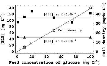
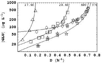
Figure 8: Growth of E. coli ML308 in a glucose-limited chemostat. (a) When the feed concentration of glucose is increased at a fixed dilution rate, the residual glucose concentration (closed symbols) is constant, and the cell density (open symbols) increases linearly (Lendenmann, 1994, Appendix B). The data for $D=0.3$ h^-1 and $D=0.6$ h^-1 is represented by the symbols, $\triangle,\blacktriangle$ and $\square,\blacksquare$, respectively. (a) When the dilution rate is increased at a fixed feed concentration (100 mg L^-1), the residual substrate concentration increases monotonically with $D$, and approaches a threshold at small dilution rates (Kovárová et al., 1996, Fig. 2). The data was obtained at 4 temperatures.

If the feed concentration is increased at a sufficiently small fixed $D$ (horizontal arrow in Fig. 7), steady growth is feasible only if the feed concentration lies in the region to the right of the blue curve, where $E_{101}$ is stable. The variation of the steady states in this region is given by (25)–(28), which imply that as the feed concentration increases, $x_{1},e_{1},\sigma_{1}$ remain constant, and $c$ increases linearly. Thus, any increase in the feed concentration is compensated by a proportional increase in the cell density — all other variables remain unchanged. We shall appeal to this fact later.

No data is available for the inducer or enzyme levels, but experiments performed with glucose-limited cultures of E. coli ML308 show that at dilution rates of $0.3$ and 0.6 h^-1, the residual substrate concentration is indeed independent of the feed concentration, and the cell density does increase linearly with the feed concentration (Fig. 8a). No threshold was observed in these experiments because the feed concentrations were relatively high ($\geq 1$ mg L^-1). As we show below, the threshold concentration for glucose is $\sim$10–50 $\mu$g L^-1.

3.2.2 Variation of steady states with $D$ at fixed $\sigma_{f,1}$

If the dilution rate is increased at any fixed $\sigma_{f,1}<\sigma_{1}^{*}$, there is no growth regardless of the dilution rate at which the chemostat is operated. If $\sigma_{f,1}>\sigma_{1}^{*}$, the variation of the steady states with $D$ is qualitatively identical to that of the Monod model: The persistence steady state, $E_{101}$, is stable for $0<D<D_{c,1}$, and the washout steady state, $E_{100}$, is stable for $D\geq D_{c,1}$ (vertical arrow in Fig. 7). We shall confine our attention to $E_{101}$, since $E_{100}$ is independent of $D$.

Variation of inducer and enzyme levels

It follows from (25)–(26) that as the dilution rate increases over the range, $(0,D_{c,1})$, the inducer level increases linearly, whereas the enzyme level passes through a maximum at $D=\sqrt{\left(Y_{1}V_{s,1}\bar{K}_{e,1}\right)k_{e,1}}.$ The latter is consistent with the data for systems with inducible enzymes (Fig. 2).

In contrast to the hypothesis of Clarke et al., the model explains the non-monotonic profile of the enzyme level as the outcome of a balance between induction and dilution/degradation (as opposed to catabolite repression). To see this, observe that the steady state enzyme level is given by the ratio of the induction and dilution/degradation rates, i.e.,

$$e_{1}=\frac{r_{e,1}^{+}}{D+k_{e,1}}.$$

Furthermore, since $x_{1}$ increases with $D$, so does $r_{e,1}^{+}$, but it saturates at sufficiently large $D$. At low values of $D$, the enzyme level increases with $D$ because the induction rate increases with $D$. At high $D$, the steady state enzyme level inversely proportional to $D$ because the induction rate saturates.

The validity of the above explanation rests upon the hypothesis that the induction rate saturates at large $D$. This hypothesis is supported by the data for the lac and ptsG operons. When batch cultures of E. coli growing exponentially on saturating concentrations of lactose (which are physiologically identical to cultures growing in a lactose-limited chemostat near the critical dilution rate) are exposed to 0.4 mM IPTG, there is almost no change in the $\beta$-galactosidase activity (Hogema et al., 1998, Table 1). Similarly, the PtsG activity of wild-type and ptsG-constitutive E. coli is the same in glucose-excess batch cultures and continuous cultures operating at high dilution rates (Seeto et al., 2004, Fig. 3). Induction is therefore already saturated during growth of E. coli on lactose or glucose, provided the dilution rate is sufficiently large. It remains to be seen if this hypothesis is also valid for the other systems. However, at large dilution rates, the enzyme activity is more or less inversely proportional to $D$ for all the systems shown Fig. 2, a result expected only if the induction rate saturates at large $D$. Thus, the decline of the enzyme activity in both constitutive mutants and wild-type cells is due to dilution, rather than catabolite repression.

Variation of the substrate concentration and cell density

According to the Monod model, the residual substrate concentration is proportional to the dilution rate, i.e., $\sigma_{1}=D/r_{g,1}^{\textnormal{max}}$, where $r_{g,1}^{\textnormal{max}}$ denotes the maximum specific growth rate on $S_{1}$ (Herbert et al., 1956). In contrast, eq. (27) yields

$$\sigma_{1}=\sigma_{1}^{*}+\left(\frac{k_{e,1}+Y_{1}V_{s,1}\bar{K}_{e,1}}{Y_{1}V_{s,1}V_{e,1}}\right)D+\left(\frac{1}{Y_{1}V_{s,1}V_{e,1}}\right)D^{2},$$

which implies that at small dilution rates, $\sigma_{1}$ approaches the threshold level, $\sigma_{1}^{*}$, and at large dilution rates, $\sigma_{1}$ is proportional to $D^{2}$. Both these properties follow from the relation, $r_{s,1}\equiv V_{s,1}e_{1}\sigma_{1}=D/Y_{1}$, and the steady state profiles of the peripheral enzyme activity. Indeed, at low dilution rates, $\sigma_{1}$ is constant because the enzyme level increases linearly. Likewise, at high dilution rates, $\sigma_{1}\sim D^{2}$ because $e_{1}\sim 1/D$.

The experiments provide clear evidence of threshold concentrations. Kovarova et al. have shown that when E. coli ML308 is grown in a glucose-limited chemostat, the residual glucose concentration approaches threshold levels of 20–40 $\mu$g/L at small dilution rates (Fig. 8b). The authors did not identify the specific mechanism underlying the threshold. It may exist, for example, simply because the maintenance requirements preclude growth. However, we shall show below that in some cases, the threshold exists precisely because the enzymes are not induced at sufficiently low values of the substrate concentration.

3.3 Mixed-substrate growth

We have shown above that in chemostats limited by a single substrate, enzyme synthesis is abolished if the feed concentration is below the threshold level, and this occurs because the induction rate of the enzyme cannot match the degradation rate. Our next goal is to show that in mixed-substrate cultures, enzyme synthesis is often abolished because the induction rate of the enzyme cannot match its dilution rate. To this end, we shall begin with the case of mixed-substrate batch cultures, where this phenomenon is particularly transparent. This analysis of batch cultures will also enable us to establish the formal similarity between the classification of the growth patterns in batch and continuous cultures.

3.3.1 Batch cultures

Mathematical classification of the growth patterns

The growth of mixed-substrate batch cultures is empirically classified based on the substrate consumption pattern (preferential or simultaneous) during the first exponential growth phase. The mathematical correlate of the foregoing empirical classification is provided by the bifurcation diagram for the equations

$$\frac{de_{1}}{dt} =V_{e,1}\frac{e_{1}\sigma_{0,1}}{\bar{K}_{e,1}+e_{1}\sigma_{0,1}}-\left(Y_{1}V_{s,1}e_{1}\sigma_{0,1}+Y_{2}V_{s,2}e_{2}\sigma_{0,2}+k_{e,1}\right)e_{1},$$ (30)

$$\frac{de_{2}}{dt} =V_{e,2}\frac{e_{2}\sigma_{0,2}}{\bar{K}_{e,2}+e_{2}\sigma_{0,2}}-\left(Y_{1}V_{s,1}e_{1}\sigma_{0,1}+Y_{2}V_{s,2}e_{2}\sigma_{0,2}+k_{e,2}\right)e_{2},$$ (31)

which describe the motion of the enzymes toward the quasisteady state corresponding to the first exponential growth phase.

We gain physical insight into the foregoing equations by observing that they are formally similar to the Lotka-Volterra model for two competing species

$$\frac{dN_{1}}{dt} =a_{1}N_{1}-\left(b_{11}N_{1}+b_{12}N_{2}\right)N_{1},$$ (32)

$$\frac{dN_{2}}{dt} =a_{2}N_{2}-\left(b_{21}N_{1}+b_{22}N_{2}\right)N_{2},$$ (33)

where $N_{i}$ is the population density of the $i$-th species; $a_{i}N_{i}$ is the (unrestricted) growth rate of the $i$-th species in the absence of any competion; and $b_{ii}N_{i}^{2}$, $b_{ij}N_{i}N_{j}$ represent the growth rate reduction due to intra- and inter-specific competition, respectively. Evidently, the net induction rate, $V_{e,i}e_{i}\sigma_{0,i}/(\bar{K}_{e,i}+e_{i}\sigma_{0,i})-k_{e,i}e_{i}$, and the two dilution terms in (30)–(31) are the correlates of the unrestricted growth rate and the two competition terms in the Lotka-Volterra model. Thus, the interaction between the enzymes is competitive (the enzymes inhibit each other via the dilution terms), despite the absence of any transcriptional repression (the induction rate of $E_{i}$ is unaffected by activity of $E_{j},j\neq i$).

Now, the Lotka-Volterra equations are known to yield coexistence or extinction steady states, depending on the values of the parameters, $b_{ij}$ (Murray, 1989). The formal similarity of eqs. (30)–(31) and (32)–(33) suggests that the enzymes will exhibit coexistence and extinction steady states, depending on the values of the physiological parameters and the initial substrate concentrations. We show below that this is indeed the case. Moreover, the coexistence and extinction steady states are the correlates of simultaneous and preferential growth, respectively.

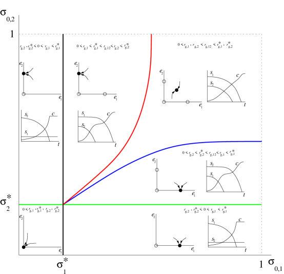
Figure 9: Bifurcation diagram classifying the growth patterns of mixed-substrate batch cultures at various initial substrate concentrations, $\sigma_{0,1}$ and $\sigma_{0,2}$. The green and black lines represent the threshold concentrations for induction of $E_{1}$ and $E_{2}$, respectively. The blue and red curves represent the locus of initial substrate concentrations defined by the equations, $r_{g,1}=r_{g,2}^{*}$ and $r_{g,2}=r_{g,1}^{*}$, respectively. The insets in each of the six regions show the dynamics at the corresponding initial substrate concentrations. The first inset shows the motion of the enzymes during the first exponential growth phase; the second one shows the resultant evolution of the substrate concentrations and cell density.

Eqs. (30)–(31) have 4 types of steady states: $e_{1}=0$, $e_{2}=0$; $e_{1}>0$, $e_{2}=0$; $e_{1}=0$, $e_{2}>0$; and $e_{1}>0$, $e_{2}>0$, which are denoted $E_{00}$, $E_{10}$, $E_{01}$, and $E_{11}$, respectively. Each of these steady states has a simple biological interpretation. If the enzyme levels reach $E_{00}$ (resp., $E_{11}$), none (resp., both) of the two substrates are consumed during the first exponential growth phase. If the enzyme levels reach $E_{10}$ (resp., $E_{01}$), only $S_{1}$ (resp., $S_{2}$) is consumed during the first exponential growth phase. The bifurcation diagram shows the existence and stability of these steady states (and hence, the growth pattern) at any given $\sigma_{0,1}$ and $\sigma_{0,2}$ (Fig. 9). It can be inferred from the following facts derived in Appendix A.

1. $E_{00}$ always exists (for all $\sigma_{0,1}$ and $\sigma_{0,2}$). It is stable if and only if

   $$r_{g,i}^{*}\equiv\frac{V_{e,i}\sigma_{0,i}}{\bar{K}_{e,i}}-k_{e,i}<0\Leftrightarrow\sigma_{0,i}<\sigma_{i}^{*},\;i=1,2$$

   i.e., the point, $\left(\sigma_{0,1},\sigma_{0,2}\right)$, lies below the green line and to the left of the black line in Fig. 9.

2. $E_{10}$ exists if and only if $\sigma_{0,1}>\sigma_{1}^{*}$, in which case it is unique, and given by

   $$e_{1}=\frac{-\left(\bar{K}_{e,1}+\frac{k_{e,1}}{Y_{1}V_{s,1}}\right)+\sqrt{\left(\bar{K}_{e,1}+\frac{k_{e,1}}{Y_{1}V_{s,1}}\right)^{2}+\frac{4\bar{K}_{e,1}r_{g,1}^{*}}{Y_{1}V_{s,1}}}}{2\sigma_{0,1}},\;e_{2}=0.$$

   At this steady state, the cells consume only $S_{1}$, and grow exponentially at the specific growth rate

   $$r_{g,1}\equiv Y_{1}V_{s,1}e_{1}\sigma_{0,1}.$$

   It is stable if and only if

   $$r_{g,2}^{*}<r_{g,1},$$ (34)

   i.e., $\left(\sigma_{0,1},\sigma_{0,2}\right)$ lies below the blue curve in Fig. 9, defined by the equation

   $$r_{g,2}^{*}=r_{g,1}.$$ (35)

   Thus, $E_{10}$ is stable under two distinct sets of conditions. Either $\sigma_{2,0}$ is below the threshold level, $\sigma_{2}^{*}$, in which case synthesis of $E_{2}$ cannot be sustained because its induction rate cannot match its degradation rate. Alternatively, $\sigma_{0,2}$ is above the threshold level, but sustained synthesis of $E_{2}$ remains infeasible because the dilution of $E_{2}$ due to growth on $S_{1}$ is too large. Thus, $r_{g,2}^{*}$ can be viewed as the highest specific growth rate tolerated by the induction machinery for $E_{2}$: Synthesis of $E_{2}$ is abolished whenever $r_{g,1}$ exceeds $r_{g,2}^{*}$. We shall refer to $r_{g,2}^{*}$ as the specific growth rate for extinction of $E_{2}$.
   For any given $\sigma_{0,1}>\sigma_{1}^{*}$, the exponential growth rate, $r_{g,1}$, can be higher or lower than $r_{g,2}^{*}$ (depending on the value of $\sigma_{0,2}$), but it cannot exceed the corresponding extinction growth rate, $r_{g,1}^{*}$. This reflects the biologically plausible fact that $e_{1}$ cannot be zero during exponential growth on $S_{1}$.

3. $E_{01}$ exists if and only if $\sigma_{0,2}>\sigma_{2}^{*}$, in which case it is (uniquely) given by the expressions

   $$e_{1}=0,\;e_{2}=\frac{-\left(\bar{K}_{e,2}+\frac{k_{e,2}}{Y_{2}V_{s,2}}\right)+\sqrt{\left(\bar{K}_{e,2}+\frac{k_{e,2}}{Y_{2}V_{s,2}}\right)^{2}+\frac{4\bar{K}_{e,2}r_{g,2}^{*}}{Y_{2}V_{s,2}}}}{2\sigma_{0,2}}.$$

   At this steady state, the cells consume only $S_{2}$, and grow exponentially at the specific growth rate

   $$r_{g,2}\equiv Y_{2}V_{s,2}e_{2}\sigma_{0,2}.$$

   It is stable if and only if

   $$r_{g,1}^{*}<r_{g,2},$$ (36)

   i.e., $\left(\sigma_{0,1},\sigma_{0,2}\right)$ lies to the left of the red curve in Fig. 9, defined by the equation

   $$r_{g,1}^{*}=r_{g,2}.$$ (37)

   Furthermore, $r_{g,2}\leq r_{g,2}^{*}$ with equality being attained precisely when $\sigma_{2}=\sigma_{2}^{*}$, in which case $r_{g,2}=r_{g,2}^{*}=0$.

4. $E_{11}$ exists and is unique if and only if $E_{10}$ and $E_{01}$ are unstable, a condition satisfied precisely when

   $$r_{g,2}^{*}>r_{g,1},\;r_{g,1}^{*}>r_{g,2},$$

   i.e., $\left(\sigma_{0,1},\sigma_{0,2}\right)$ lie between the blue and red curves in Fig. 9. At this steady state, both enzymes “coexist” because neither substrate supports a specific growth rate that is large enough to annihilate the enzymes for the other substrate. Hence, both substrates are consumed, and the cells grow exponentially at the specific growth rate

   $$r_{g,12}\equiv Y_{1}V_{s,1}e_{1}\sigma_{0,1}+Y_{2}V_{s,2}e_{2}\sigma_{0,2},$$

   where $e_{1},e_{2}$ are the unique positive solutions of (30)–(31).

5. The blue curve and red curves are given by the equations

   $$r_{g,1}^{*} =\left(1+\frac{k_{e,1}}{Y_{1}V_{s,1}\bar{K}_{e,1}}\right)r_{g,2}^{*}+\frac{1}{Y_{1}V_{s,1}\bar{K}_{e,1}}\left(r_{g,2}^{*}\right)^{2},$$ (38)

   $$r_{g,2}^{*} =\left(1+\frac{k_{e,2}}{Y_{2}V_{s,2}\bar{K}_{e,2}}\right)r_{g,1}^{*}+\frac{1}{Y_{2}V_{s,2}\bar{K}_{e,2}}\left(r_{g,2}^{*}\right)^{2},$$ (39)

   respectively. Both equations define graphs of increasing functions passing through $(\sigma_{1}^{*},\sigma_{2}^{*})$, but the blue curve always lies below the red curve.

Thus, the bifurcation diagram consists of 6 distinct regions such that exactly one of the four steady states is stable in each region.

The bifurcation diagram implies that there are six possible growth patterns, depending on the initial substrate concentrations. Three of these growth patterns occur if $\sigma_{0,1}<\sigma_{1}^{*}$ or/and $\sigma_{0,1}<\sigma_{2}^{*}$. If both $\sigma_{0,1}$ and $\sigma_{0,2}$ are below their respective threshold concentrations, neither substrate is consumed. If only one of them is below its threshold level, say, $\sigma_{0,2}<\sigma_{2}^{*}$, only $S_{1}$ is consumed during the first exponential growth phase. However, growth is not diauxic because $S_{2}$ is never consumed. If $\sigma_{0,1}>\sigma_{1}^{*}$ and $\sigma_{0,2}>\sigma_{2}^{*}$, the model predicts the existence of three additional growth patterns.

1. If $\sigma_{0,1}$, $\sigma_{0,2}$ lie in the region between the blue and green curves, $e_{2}$ approaches zero during the first exponential growth phase. Importantly, since $\sigma_{0,2}$ is higher than the threshold level, $E_{2}$ is synthesized upon exhaustion of $S_{1}$ at the end of the first exponential growth phase. Hence, growth is diauxic with preferential consumption of $S_{1}$.

2. If $\sigma_{0,1}$, $\sigma_{0,2}$ lie in the region between the red and black curves, $e_{1}$ approaches zero during the first exponential growth phase, i.e., there is diauxic growth with preferential consumption of $S_{2}$.

3. If $\sigma_{0,1}$, $\sigma_{0,2}$ lie between the red and blue curves, $e_{1}$ and $e_{2}$ attain positive values during the first exponential growth phase. Consequently, both substrates are consumed until one of them is exhausted, and there is no diauxic lag before the remaining substrate is consumed.

We show below that the foregoing classification is consistent with the data.

Growth patterns at saturating substrate concentrations

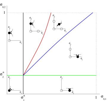
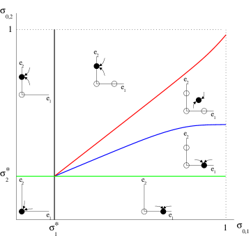
Figure 10: Bifurcation diagrams corresponding to diauxic growth under substrate-excess conditions ($\sigma_{0,1},\sigma_{0,2}\approx 1$). (a) Preferential consumption of $S_{1}$. (b) Preferential consumption of $S_{2}$.

Physiological experiments, which are generally performed with saturating substrate concentrations ($\sigma_{0,1},\sigma_{0,2}\approx 1$), show that depending on the cell type, the two substrates are consumed sequentially or simultaneously. The behavior of the model is consistent with this observation. To see this, observe that depending on the values of the physiological parameters (which, in effect, determine the cell type), there are three possible arrangements of the red and blue curves, each of which yields a distinct growth pattern at saturating substrate concentrations. Indeed, $S_{1}$ is consumed preferentially if $(1,1)$ lies below the blue curve (Fig. 10a). This occurs precisely when the physiological parameters satisfy the condition

$$\frac{V_{e,1}}{\bar{K}_{e,1}} >\frac{V_{e,2}}{\bar{K}_{e,2}}+\frac{1}{Y_{1}V_{s,1}\bar{K}_{e,1}}\left(\frac{V_{e,2}}{\bar{K}_{e,2}}\right)^{2},$$ (40)

obtained from (38) by neglecting enzyme degradation ($k_{e,i}=0$). Likewise, $S_{2}$ is consumed preferentially if $(1,1)$ lies above the red curve (Fig. 10b), i.e., the physiological parameters satisfy the condition

$$\frac{V_{e,2}}{\bar{K}_{e,2}} >\frac{V_{e,1}}{\bar{K}_{e,1}}+\frac{1}{Y_{2}V_{s,2}\bar{K}_{e,12}}\left(\frac{V_{e,1}}{\bar{K}_{e,1}}\right)^{2},$$ (41)

obtained from (39) upon setting $k_{e,i}=0$. Finally, the substrates are consumed simultaneously if (1,1) lies above the blue curve and below the red curve (Fig. 9), i.e., both the foregoing conditions are violated.

The biological meaning of these conditions was discussed in earlier work (Narang and Pilyugin, 2007a). Indeed, one can check that (40) and (41) are equivalent to the conditions

$$\alpha <\alpha_{*}\equiv\frac{\kappa_{2}\left(-\kappa_{1}+\sqrt{\kappa_{1}^{2}+4}\right)}{2},$$

$$\alpha >\alpha^{*}\equiv\frac{2}{\kappa_{1}\left(-\kappa_{2}+\sqrt{\kappa_{1}^{2}+4}\right)},$$

respectively, where $\alpha\equiv\sqrt{Y_{2}V_{s,2}V_{e,2}}/\sqrt{Y_{1}V_{s,1}V_{e,1}}$ is a measure of the maximum specific growth rate on $S_{2}$ relative to that on $S_{1}$, and $\kappa_{i}\equiv\bar{K}_{e,i}/\sqrt{V_{e,i}/(Y_{i}V_{s,i})}$ is a measure of saturation constant for induction of $E_{i}$. Thus, the substrates are consumed preferentially whenever the maximum specific growth rate on one of the substrates is sufficiently large compared to that on the other substrate. Just how large this ratio must be depends on the saturation constants, $\kappa_{i}$. Enzymes with small saturation constants are quasi-constitutive — their synthesis cannot be abolished even if the other substrate supports a large specific growth rate. In contrast, synthesis of enzymes with large saturation constants can be abolished even if the other substrate supports a comparable specific growth rate.

Transitions triggered by changes in substrate concentrations

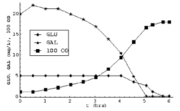
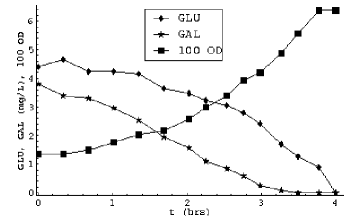
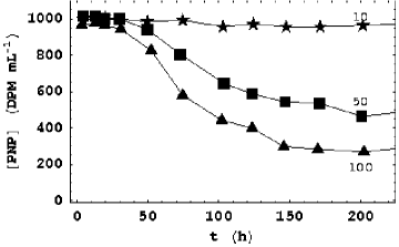
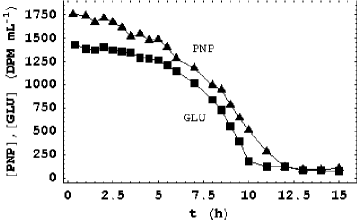
Figure 11: Transitions of the growth patterns triggered by changes in the initial substrate concentrations. Upper panel: Batch growth of Escherichia coli ML308 on mixtures of glucose and galactose. (a) At high initial glucose concentrations (20 mg L^-1), glucose is consumed before galactose (Lendenmann, 1994). (b) At low initial glucose concentrations (5 mg L^-1), glucose and galactose are consumed simultaneously (Egli et al., 1993, Fig. 1). Lower panel: Batch growth of Pseudomonas on PNP and PNP + glucose (Schmidt et al., 1987, Figs. 1,4). DPM denotes disintegrations per min of ¹⁴C-labelled PNP and glucose. (c) No PNP is consumed if its initial concentration is 10 $\mu$g L^-1. Significant consumption occurs at initial concentrations of 50 and 100 $\mu$g L^-1. (d) PNP and glucose are consumed simultaneously if their initial concentrations are high (3 and 10 mg L^-1, respectively).

Figs. 9–10 imply that the growth pattern can be changed by altering the initial substrate concentrations. We show below that this conclusion is consistent with the data.

As a first example, consider a cell type that prefers to consume $S_{1}$ under substrate-excess conditions ($\sigma_{0,1},\sigma_{0,2}\approx 1$). Its growth pattern at any $\sigma_{0,1}$, $\sigma_{0,2}$ is then described by Fig. 10a, which implies that if $\sigma_{0,1}$ is decreased sufficiently from 1, both substrates will be consumed simultaneously. Such behavior has been observed in experiments. If the initial concentrations of glucose and galactose are 20 mg/L and 5 mg/L, respectively, E. coli ML308 consumes glucose before galactose (Fig. 11a). If the initial concentration of glucose is reduced to 5 mg/L or lower, glucose and galactose are consumed simultaneously (Fig. 11b).

The data in Figs. 11a,b are open to question because the initial cell densities are so large ($\sim 10^{9}$ cells L^-1) that the substrates may have been exhausted before the enzymes reached the quasisteady state corresponding to balanced growth. However, similar results have also been obtained in studies performed with very small initial cell densities ($10^{3}$–$10^{5}$ cells L^-1). Indeed, Schmidt and Alexander observed that “simultaneous use of two substrates is concentration dependent … Pseudomonas sp. ANL 50 mineralized glucose and aniline simultaneously when present at 3 $\mu$g L^-1 but metabolized them diauxically at 300 $\mu$g L^-1” (Schmidt and Alexander, 1985, Figs. 3–4). Likewise, Pseudomonas acidovorans consumed acetate before phenol when the concentrations of these substrates were >70 and 2 $\mu$g L^-1, respectively. If the initial concentration of acetate was reduced to 13 $\mu$g L^-1, both substrates were consumed simultaneously.

In terms of the model, these transitions from sequential to simultaneous substrate consumption can be understood as follows. Sequential substrate consumption occurs at high concentrations of the preferred substrate because it supports such a large specific growth rate that the enzymes associated with the secondary substrate are diluted to extinction. Reducing the initial concentration of the preferred substrate decreases its ability to support growth, and thus dilute the secondary substrate enzymes to extinction. Consequently, both substrates are consumed.

The growth of Pseudomonas sp. on p-nitrophenol (PNP) and glucose furnishes additional examples of growth pattern transitions driven by changes in the initial substrate concentrations. Schmidt et al. found that no PNP was consumed if its initial concentration was 10 $\mu$g L^-1, and significant mineralization occurred at the higher initial concentrations of 50 and 100 $\mu$g L^-1 (Fig. 11c). It follows that the threshold concentration for PNP lies between 10 and 50 $\mu$g L^-1. Importantly, the addition of 20 mg L^-1 glucose to a culture containing 10 $\mu$g L^-1 PNP failed to stimulate PNP consumption. The authors concluded that “the threshold was not a result of the fact that the concentration of PNP was too low to meet maintenance energy requirements of the organism, but rather supports the hypothesis that the concentration was too low to induce degradative enzymes.” Finally, it was observed that when the initial concentrations of PNP and glucose were increased to saturating levels of 3 mg L^-1 and 10 mg L^-1, respectively, both substrates were consumed simultaneously (Fig. 11d). All these results are consistent with the bifurcation diagram shown in Fig. 9.

Figs. 9–10 extend the results obtained in Narang and Pilyugin, 2007a. There, we constructed bifurcation diagrams describing the variation of the growth patterns in response to changes in the physiological parameters at (fixed) saturating substrate concentrations. These genetic bifurcation diagrams explained the phenotypes of many different mutants and recombinant cells. Figs. 9–10 can be viewed as epigenetic bifurcation diagrams, since they describe the variation of the growth pattern when a given cell type, characterized by fixed physiological parameters, is exposed to various initial substrate concentrations.

3.3.2 Continuous cultures

In the experimental literature, the growth pattern of mixed-substrate continuous cultures is classified based on the manner in which the two substrates are consumed when the dilution rate is increased at a given pair of feed concentrations. Either both substrates are consumed at all dilution rates up to washout, or both substrates are consumed up to an intermediate dilution rate beyond which only one of the substrates is consumed. We show below that the model predicts these growth patterns. Moreover, it can quantitatively capture the variation of the steady state enzyme levels, substrate concentrations, and cell density with respect to the dilution rate and the feed concentrations.

Mathematical classification of the growth patterns

The mathematical correlate of the experimentally observed growth patterns corresponds to the bifurcation diagram for eqs. (8)–(12), which describes the existence and stability of the steady states in the 3-dimensional $\sigma_{f,1},\sigma_{f,2},D$-space.

Table 1: Necessary and sufficient conditions for existence and stability of the steady states for mixed-substrate growth in continuous cultures (see Appendix C for details).

Steady	Defining	Biological	Existence	Stability
state	property	meaning	condition(s)	condition(s)
$E_{000}$	$e_{1}=0,e_{2}=0,$	No substrate	Always	$D_{t,1}<0,$
	$c=0$	consumed	exists	$D_{t,2}<0$
$E_{101}$	$e_{1}>0,e_{2}=0,$	Only $S_{1}$	$D_{t,1}>0,$	$D>D_{t,2}$
	$c>0$	consumed	$0<D<D_{c,1}$
$E_{100}$	$e_{1}>0,e_{2}=0,$	Washout	$D_{t,1}>0$	$D_{t,2}<D_{c,1},$
	$c=0$	of $E_{101}$		$D>D_{c,1}$
$E_{011}$	$e_{1}=0,e_{2}>0$	Only $S_{2}$	$D_{t,2}>0,$	$D>D_{t,1}$
	$c>0$	consumed	$0<D<D_{c,2}$
$E_{010}$	$e_{1}=0,e_{2}>0,$	Washout	$D_{t,2}>0$	$D_{t,1}<D_{c,2},$
	$c=0$	of $E_{011}$		$D>D_{c,2}$
$E_{111}$	$e_{1}>0,e_{2}>0,$	Both $S_{1},S_{2}$	$D_{t,1},D_{t,2}>0,$	Whenever it
	$c>0$	consumed	$D<D_{t,1},D_{t,2},D_{c}$	exists
$E_{110}$	$e_{1}>0,e_{2}>0,$	Washout	$D_{t,2}>D_{c,1}$,	$D>D_{c}$
	$c=0$	of $E_{111}$	$D_{t,1}>D_{c,2}$

Eqs. (8)–(12) have 7 steady states, but 5 of them are “single-substrate steady states” (see rows 1–5 of Table 1). Indeed, $E_{000}$, $E_{101}$, and $E_{100}$ (resp., $E_{000}$, $E_{011}$, and $E_{010}$) are observed in chemostats limited by $S_{1}$ (resp., $S_{2}$). Their existence in mixed-substrate growth implies that even if both substrates are supplied to the chemostat, there are steady states at which only one of the substrates is consumed. We shall see below that these steady states can become stable under certain conditions. Here, it suffices to observe that only two of 7 steady states, namely, $E_{111}$ ($e_{1}>0$, $e_{2}>0$, $c>0$) and $E_{110}$ ($e_{1}>0$, $e_{2}>0$, $c>0$), are uniquely associated with mixed-substrate growth. They correspond to simultaneous consumption of both substrates and its washout.

The existence and stability of the steady states are completely determined by five special dilution rates, namely, $D_{t,i}$, $D_{c,i}$, and $D_{c}$ (Table 1, columns 4–5). These dilution rates are the analogs of the special specific growth rates considered in the analysis of batch cultures. Indeed, the transition dilution rate for $S_{i}$,

$$D_{t,i}\equiv\frac{V_{e,i}\sigma_{f,i}}{\bar{K}_{e,i}}-k_{e,i},$$ (42)

is the analog of the extinction growth rate, $r_{g,i}^{*}$. It is the maximum dilution rate up to which synthesis of $E_{i}$ can be sustained. The critical dilution rate, $D_{c,i}$, given by the relation

$$D_{c,i}=Y_{i}V_{s,i}\frac{-\left(\bar{K}_{e,i}+\frac{k_{e,i}}{Y_{i}V_{s,i}}\right)+\sqrt{\left(\bar{K}_{e,i}+\frac{k_{e,i}}{Y_{i}V_{s,i}}\right)^{2}+\frac{4K_{e,i}D_{t,i}}{Y_{1}V_{s,i}}}}{2},$$

is the analog of $r_{g,i}$. It is the maximum dilution rate up to which growth can be sustained in a chemostat supplied with only $S_{i}$, and satisfies the relation, $D_{ci}\leq D_{t,i}$ with equality being obtained precisely when $\sigma_{i}=\sigma_{i}^{*}$, in which case, $D_{c,i}=D_{t,i}=0$ (see dashed and blue lines in Fig. 7). Finally, the critical dilution rate, $D_{c}$, is defined as

$$D_{c}\equiv Y_{1}V_{s,1}e_{1}\sigma_{f,1}+Y_{2}V_{s,2}e_{2}\sigma_{f,2},$$

where $e_{1},e_{2}$ are the unique positive steady state solutions of (30)–(31) with $\sigma_{0,i}$ replaced by $\sigma_{f,i}$. It is the analog of the function, $r_{g,12}$. Thus, $r_{g,i}^{*}$, $r_{g,i}$, $r_{g,12}$, and their analogs, $D_{t,i}$, $D_{c,i}$, $D_{c}$, are defined by formally identical expressions, the only difference being that $\sigma_{0,i}$ is replaced by $\sigma_{f,i}$.

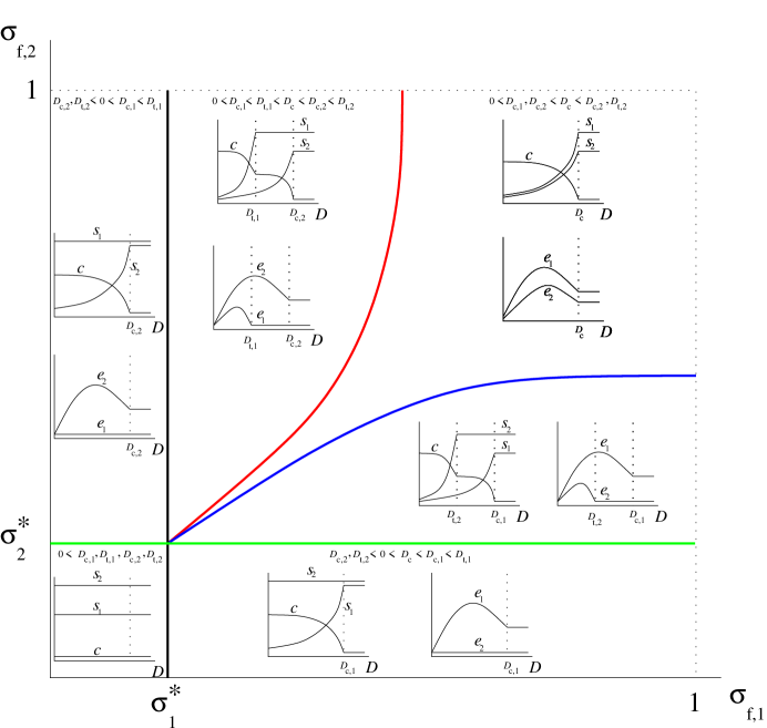
Figure 12: Bifurcation diagram classifying the growth patterns of mixed-substrate continuous cultures at various feed concentrations, $\sigma_{f,1}$ and $\sigma_{f,2}$. The green and black lines represent the threshold concentrations for induction of $E_{1}$ and $E_{2}$, respectively. The blue and red curves represent the locus of initial substrate concentrations defined by the equations, $D_{c,1}=D_{t,2}$ and $D_{c,2}=D_{t,1}$, respectively. The insets in each of the six regions show the variation of the steady states with $D$ at the corresponding feed concentrations.

The formal similarity of the expressions for $D_{t,i}$, $D_{c,i}$, $D_{c}$ and $r_{g,i}^{*}$, $r_{g,i}$, $r_{g,12}$ implies that for a given set of physiological parameters, the relations, $\sigma_{f,i}=\sigma_{i}^{*}$, $D_{t,1}=D_{c,2}$ and $D_{t,2}=D_{c,1}$, define curves on the $\sigma_{f,1},\sigma_{f,2}$-plane that are identical to the curves on the $\sigma_{0,1},\sigma_{0,2}$-plane defined by the equations, $\sigma_{0,i}=\sigma_{i}^{*}$, $r_{g,1}^{*}=r_{g,2}$ and $r_{g,2}^{*}=r_{g,1}$. It follows that the relations, $\sigma_{f,i}=\sigma_{i}^{*}$, $D_{t,1}=D_{c,2}$, $D_{t,2}=D_{c,1}$, determine a partitioning of the $\sigma_{f,1},\sigma_{f,2}$-plane into 6 regions, which is identical to the partitioning of the bifurcation diagram for batch cultures, the only difference being that the coordinates are $\sigma_{f,1},\sigma_{f,2}$, rather than $\sigma_{0,1},\sigma_{0,2}$ (Fig. 12).

Each of the six regions in Fig. 12 corresponds to unique growth pattern that can be inferred from the existence and stability properties summarized in columns 4–5 of Table 1. For instance, if $\left(\sigma_{f,1},\sigma_{f,2}\right)$ lies in the region between the green and blue curves in Fig. 12, both substrates are consumed for all $0<D<D_{t,2}$, only $S_{1}$ is consumed for all $D_{t,2}\leq D<D_{c,1}$, and neither substrate is consumed because the cells are washed out for all $D\geq D_{c,1}$. To see this, observe that in the region of interest (between the green and blue curves), the special dilution rates stand in the relation

$$0<D_{c,2}<D_{t,2}<D_{c}<D_{c,1}<D_{t,1}.$$

The existence and stability conditions listed in Table 1 therefore imply that as $D$ increases, 4 of the 7 steady states play no role because they are unstable whenever they exist, or do not exist at all. Indeed:

1. $E_{000}$ and $E_{010}$ exist at all $D>0$, but they are always unstable because the stability conditions for these two steady states ($D_{t,1},D_{t,2}>0$ and $D_{t,1}<D_{c,2}$, respectively) are violated in the region of interest .

2. $E_{011}$ exists for all $0<D<D_{c,2}$, but it is unstable whenever it exists because the stability condition, $D>D_{t,1}$, is not satisfied in the region of interest.

3. $E_{110}$ does not exist at all since one of the existence conditions, $D_{t,2}>D_{c,1}$, is violated in the region of interest.

It follows that only the remaining three steady states are relevant. One can check by appealing to Table 1 that $E_{111}$ is stable for $0<D<D_{t,2}$, $E_{101}$ is stable for $D_{t,2}<D<D_{c,1}$, and $E_{100}$ is stable for $D>D_{c,1}$. Hence, both substrates are consumed for all $0<D<D_{t,2}$. At $D=D_{t,2}$, $e_{2}$ becomes zero. Only $S_{1}$ is consumed for all $D_{t,2}\leq D<D_{c,1}$ until $c$ becomes zero at $D=D_{c,1}$. Neither substrate is consumed for $D>D_{c,1}$.

Similar arguments, applied to all the regions in Fig. 12, show that there are 6 distinct growth patterns. Three of these growth patterns occur when at least one of the feed concentrations is below its threshold level.

1. If both feed concentrations are below the threshold level, $E_{000}$ is always stable, so that neither substrate is consumed at any dilution rate.

2. If $\sigma_{f,2}<\sigma_{2}^{*}$, but $\sigma_{f,1}>\sigma_{1}^{*}$, $E_{101}$ is stable (i.e., only $S_{1}$ is consumed) for all $0<D<D_{c,1}$, and $E_{100}$ is stable (i.e., the cells wash out) whenever $D\geq D_{c,1}$. This is qualitatively similar to the behavior observed during single-substrate growth on $S_{1}$ (Fig. 7). Thus, if the feed concentration of $S_{2}$ is at sub-threshold levels, it has no effect on the behavior of the chemostat.

3. If $\sigma_{f,1}<\sigma_{1}^{*}$, and $\sigma_{f,2}>\sigma_{2}^{2}$, $E_{011}$ is stable (i.e., only $S_{2}$ is consumed) for all $0<D<D_{c,2}$, and $E_{010}$ is stable (i.e., the cells wash out) for $D\geq D_{c,2}$. This is qualitatively similar to the behavior of the chemostat during single-substrate growth on $S_{2}$.

If both feed concentrations are above their respective threshold levels, there are three additional growth patterns.

1. If $\sigma_{f,1}$ and $\sigma_{f,2}$ lie between the red and blue curves, $E_{111}$ (i.e., both substrates are consumed) for $0<D<D_{c}$, and $E_{110}$ is stable (i.e., cells wash out) for $D\geq D_{c}$. Thus, both substrates are consumed at all dilution rates up to washout.

2. If $\sigma_{f,1}$ and $\sigma_{f,2}$ lie between the green and blue curves, $E_{111}$ is stable (i.e., both substrates are consumed) for all $0<D<D_{t,2}$, $E_{101}$ is stable (i.e., only $S_{1}$ is consumed) for all $D_{t,1}\leq D<D_{c,1}$, and $E_{100}$ is stable (the cells wash out) for all $D>D_{c,1}$.

3. If $\sigma_{f,1}$ and $\sigma_{f,2}$ lie between the black and red curves, $E_{111}$ is stable (i.e., both substrates are consumed) for all $0<D<D_{t,1}$, $E_{011}$ is stable (i.e., only $S_{2}$ is consumed) for all $D_{t,2}\leq D<D_{c,2}$, and $E_{100}$ is stable (the cells wash out) for all $D>D_{c,2}$.

These growth patterns are the mathematical correlates of the growth patterns shown in Fig. 3.

The model predicts that the growth pattern in continuous cultures can be changed by altering the feed concentrations. Unfortunately, there is no experimental data at subsaturating feed concentrations ($\sigma_{f,i}\lesssim K_{s,i}$) due to technical difficulties associated with wall growth. Henceforth, we shall confine our attention to growth at saturating feed concentrations ($\sigma_{f,i}\approx 1$).

We have shown above that for a given cell type, the bifurcation diagrams for batch and continuous cultures are formally identical — one can be generated from the other by a mere relabeling of the coordinate axes. This formal identity provides a precise mathematical explanation for the empirically observed correlation between the batch and continuous growth patterns of a given cell type. To see this, suppose the cells in question consume $S_{1}$ preferentially in substrate-excess batch cultures ($\sigma_{0,i}\approx 1$). The bifurcation diagram for this system then has the form shown in Fig. 10a. The continuous growth patterns of this system are given by the very same figure, the only difference being that the coordinates, $\sigma_{0,1}$, $\sigma_{0,2}$, are replaced by $\sigma_{f,1}$, $\sigma_{f,2}$, respectively. It follows that if the cells are grown in continuous cultures fed with saturating substrate concentrations ($\sigma_{f,i}\approx 1$), they will consume both substrates at low dilution rates, and only $S_{1}$ at all high dilution rates up to washout (Fig. 3b). A similar argument shows that if the cells consume both substrates in substrate-excess batch culture (bifurcation diagram given by a relabeled Fig. 9), their growth in continuous cultures will be such that both substrates are consumed at all dilution rates up to washout (Fig. 3a).

The model predicts the observed variation of the steady states with $D$ and $s_{f,i}$

Although the model predicts the existence of the observed growth patterns, it remains to determine if the variation of the steady states with $D$ and $s_{f,i}$ is in quantitative agreement with the data. Since the variation of the “single-substrate steady states” with $D$ and $s_{f,i}$ is consistent with the data (Section 3.2), it suffices to focus on $E_{111}$, the only growth-supporting steady state uniquely associated with mixed-substrate growth. This steady state can be observed in systems exhibiting both the simultaneous and the preferential growth patterns. However, since the data for simultaneous systems is limited, we shall focus on preferential systems. In our discussion of these systems, we shall assume, furthermore, that $S_{1}$ is the “preferred” substrate. This entails no loss of generality since the equations for $S_{1}$ and $S_{2}$ (and the associated physiological variables) are formally identical: Interchanging the indices does not change the form of the equations.

Two types of experiments can be found in the literature.

1. Either the dilution rate was changed at fixed feed concentrations.

2. Alternatively, the mass fraction of the substrates in the feed, $\psi_{i}\equiv s_{f,i}/(s_{f,1}+s_{f,2})$, was changed at fixed total feed concentration, $s_{f,t}\equiv s_{f,1}+s_{f,2}$, and (sufficiently small) dilution rate.

The model predicts that in the first case, $E_{111}$ is stable at all dilution rates below $D_{t,2}$, the transition dilution rate for the “less preferred” substrate. In the second case, $E_{111}$ is stable at all feed fractions, except those near the extreme values, 0 and 1, where the model predicts threshold effects. Such threshold effects have been observed when the feed contained a very small fraction of one of the substrates (Kovar et al., 2002; Ng and Dawes, 1973; Rudolph and Grady, 2002). Nevertheless, we shall restrict our attention to intermediate values of $\psi_{i}$ at which $E_{111}$ is the stable steady state.

The steady state, $E_{111}$, satisfies the equations

$$0 =D(s_{f,i}-s_{i})-r_{s,i}c,$$ (43)

$$0 =V_{e,i}\frac{\sigma_{i}}{\bar{K}_{e,i}+e_{i}\sigma_{i}}-\left(D+k_{e,i}\right),$$ (44)

$$0 =Y_{1}r_{s,1}+Y_{2}r_{s,2}-D,$$ (45)

$$x_{i} \approx\frac{r_{s,i}}{k_{x,i}}.$$ (46)

These equations do not yield an analytical solution valid for all $D$ and $s_{f,i}$. However, we show below that they can be solved for the two limiting cases of low and high $D$, from which the entire solution can be pieced together.

Before considering these limiting cases, it is useful to note that eqs. (43) and (45) imply that

$$c =Y_{1}\left(s_{f,1}-s_{1}\right)+Y_{2}\left(s_{f,2}-s_{2}\right),$$ (47)

$$\frac{Y_{i}r_{s,i}}{D} =\beta_{i}\equiv\frac{Y_{i}(s_{f,i}-s_{i})}{Y_{1}(s_{f,1}-s_{1})+Y_{2}(s_{f,2}-s_{2})}.$$ (48)

The first relation says that the steady state cell density is the sum of the cell densities derived from the two substrates. The second relation states that $\beta_{i}$, the fraction of biomass derived from $S_{i}$, equals the fraction of the total specific growth rate, $D$, supported by $S_{i}$. Evidently, $\beta_{i}\leq 1$ with equality being attained only during single-substrate growth.

Eq. (48) immediately yields

$$r_{s,i}=\frac{\beta_{i}D}{Y_{i}},$$ (49)

which explains the following well-known empirical observation: At any given $D$, the mixed-substrate specific uptake rate of $S_{i}$ is always lower than the single-substrate specific uptake rate of $S_{i}$ (reviewed in Egli, 1995). This correlation is a natural consequence of the mass balances for the substrates and cells, together with the constant yield property. The mixed-substrate specific uptake rate is smaller simply because both substrates are consumed to support the specific growth rate, $D$, whereas only one substrate supports the very same specific growth rate during single-substrate growth.

Low dilution rates

The first limiting case corresponds to dilution rates so small that both substrates are at subsaturating levels, i.e., $s_{i}\lesssim K_{s,i}\ll s_{f,i}$. Since both substrates are almost completely consumed, (47)–(48) become

$$c \approx Y_{1}s_{f,1}+Y_{2}s_{f,2},$$ (50)

$$r_{s,i} =\frac{\beta_{i}D}{Y_{i}},\;\beta_{i}\approx\frac{Y_{i}s_{f,i}}{Y_{1}s_{f,1}+Y_{2}s_{f,2}}=\frac{Y_{i}\psi_{i}}{Y_{1}\psi_{1}+Y_{2}\psi_{2}}.$$ (51)

Evidently, $\beta_{i}$ is completely determined by $\psi_{i}$, the fraction of $S_{i}$ in the feed. Moreover, $\beta_{i}(\psi_{i})$ is an increasing function of $\psi_{i}$ with $\beta_{i}(0)=0$ and $\beta_{i}(1)=1$. It is identical to $\psi_{i}$ when the yields on both substrates are the same.

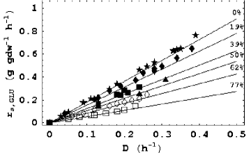
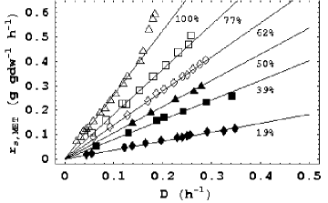
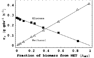
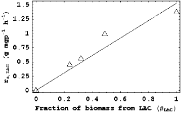
Figure 13: Upper panel: The specific substrate uptake rate increases linearly when the dilution rate is increased at fixed feed concentrations. Specific uptake rates of (a) glucose and (b) methanol during growth of H. polymorpha on various mixtures of glucose and methanol (Egli et al., 1986, Figs. 4–5). The percentages show the percent methanol in the feed. The total feed concentration of glucose and methanol was 5 g L^-1. Lower panel: If the fraction of $S_{i}$ in the feed is increased at a fixed dilution rate, the specific substrate uptake rate increases linearly with $\beta_{i}$. (c) Growth of H. polymorpha on a mixture of glucose and methanol at $D=0.145$ h^-1 (Egli et al., 1982b, Fig. 5). (d) Growth of E. coli K12 on various mixtures of lactose and glucose at $D=0.4$ h^-1 (calculated from Fig. 4 of Smith and Atkinson, 1980). The lines in the figures show the specific substrate uptake rates predicted by eq. (51) with the experimentally measured single-substrate yields, $Y_{\textnormal{GLU}}=0.55$, $Y_{\textnormal{MET}}=0.38$ in (a)–(c), and $Y_{\textnormal{GLU}}=Y_{\textnormal{LAC}}$ in (d).

Eq. (51) implies that if $D$ is increased at fixed feed concentrations, $r_{s,i}$ increases linearly. Likewise, if $\psi_{i}$, and hence, $\beta_{i}$, is increased at a fixed dilution rate, $r_{s,i}$ increases linearly with $\beta_{i}$. Both conclusions are consistent with the data. Fig. 13 shows that eq. (51) provides excellent fits to the data for growth of H. polymorpha on glucose + methanol and E. coli on glucose + lactose. The validity of (51) at low dilution rates has been demonstrated for many different systems (reviewed in Kovarova-Kovar and Egli, 1998).

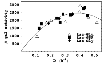
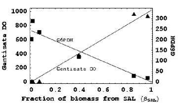
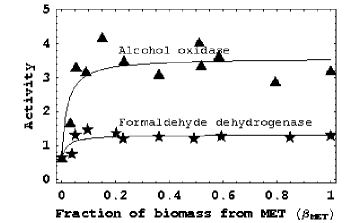
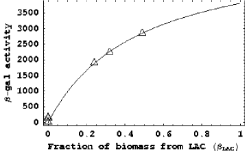
Figure 14: Variation of the peripheral enzyme levels: (a) Activity of $\beta$-galactosidase during growth of E. coli K12 on mixtures of lactose (1mM) plus glucose (2mM), glucose-6-phosphate (2mM), or glycerol (4mM) (Smith and Atkinson, 1980, Fig. 3). (b) Activity of gentisate-1,2-dioxygenase and glucose-6-phosphate dehydrogenase (G6PDH) during growth of P. aeruginosa on salicylate + glucose at $D=0.02$ h^-1 (Rudolph and Grady, 2002, Fig. 3). (c) Activities of alcohol oxidase and formaldehyde dehydrogenase during growth of H. polymorpha on various mixtures of glucose and methanol at $D=0.15$ h^-1 and $s_{f,t}=5$ g L^-1 (Egli et al., 1982b, Figs. 7A,C). (d) Activity of $\beta$-galactosidase during growth of E. coli K12 on various mixtures of lactose and glucose at $D=0.4$ h^-1 (calculated from Fig 5 of Smith and Atkinson, 1980).

The physiological variables, $x_{i}$ and $e_{i}$, are completely determined by the specific uptake rate of $S_{i}$. Indeed, (46) and (44) imply that

$$x_{i} \approx\frac{r_{s,i}}{k_{x,i}}=\frac{\beta_{i}D}{Y_{i}k_{x,i}},$$ (52)

$$e_{i} =\frac{V_{e,i}}{D+k_{e,i}}\frac{\beta_{i}D}{Y_{i}V_{s,i}\bar{K}_{e,i}+\beta_{i}D}.$$ (53)

It follows from (53) that:

1. If the dilution rate is increased at fixed feed concentrations, the steady state enzyme level passes through a maximum. However, at every dilution rate, the mixed-substrate enzyme level is always lower than the single-substrate enzyme level.

2. If the fraction of $S_{i}$ in the feed is increased at a fixed dilution rate, the activity of $E_{i}$ increases with $\beta_{i}$. The increase is linear if $D$ is small, and hyperbolic if $D$ is large.

Both results are consistent with the data (Fig. 14).

Based on studies with batch cultures of E. coli, it is widely believed that glucose and glucose-6-phosphate (G6P) are strong inhibitors of $\beta$-galactosidase synthesis, whereas glycerol is a weak inhibitor. It is therefore remarkable that the $\beta$-galactosidase activity at any given dilution rate is the same in three different continuous cultures fed with lactose + glucose, lactose + G6P, and lactose + glycerol (Fig. 14a). The model provides a simple explanation for this data. To see this, let $S_{1}$ and $S_{2}$ denote lactose and glucose/G6P/glycerol, respectively. Now, (53) implies that any given dilution rate, the influence of $S_{2}$ on the $\beta$-galactosidase activity, $e_{1}$, is completely determined by the parameter,

$$\beta_{1}\approx\frac{Y_{1}s_{f,1}}{Y_{1}s_{f,1}+Y_{2}s_{f,2}},$$

which is identical to $\psi_{1}$, the mass fraction of lactose in the feed, because the yields on lactose, glucose, G6P, and glycerol are similar. It turns out that the feed concentrations used in the experiments were such that $\psi_{1}\approx 0.45$ in all the experiments. Consequently, the $\beta$-galactosidase activity at any $D$ is independent of the chemical identity of $S_{2}$.

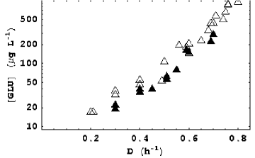
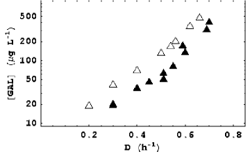
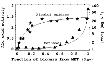
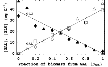
Figure 15: Upper panel: Variation of the glucose and galactose concentrations with the dilution rate during single- and mixed-substrate growth of E. coli ML308 on glucose or/and galactose (Lendenmann, 1994; Lendenmann et al., 1996, Appendix B). The residual concentrations of (a) glucose and (b) galactose during mixed-substrate growth ($\blacktriangle$) are lower than the corresponding levels during single-substrate growth ($\vartriangle$). Lower panel: The relationship between the substrate concentration and the peripheral enzyme level. (a) Growth of C. boidinii on various mixtures of methanol and glucose at $D=0.14$ h^-1 and $s_{f,t}=5.0$ g L^-1 (Egli et al., 1993, Fig. 7). When the activity of alcohol oxidase increases ($0\leq\beta_{\textnormal{MET}}\lesssim 0.4$), the methanol concentration is constant. When the activity of alcohol oxidase saturates ($\beta_{\textnormal{MET}}\gtrsim 0.4$), the methanol concentration increases. (b) Residual concentrations of galactose (open symbols) and glucose (closed symbols) during growth on E. coli ML308 on various mixtures of galactose and glucose at $D=0.3$ h^-1 and $s_{f,t}=1$ ($\vartriangle,\blacktriangle$), 10 ($\lozenge,\blacklozenge$), and 100 ($\square$) mg L^-1 (Lendenmann, 1994; Lendenmann et al., 1996).

The steady state substrate concentrations are given by the expression

$$\sigma_{i}=\frac{r_{s,i}}{V_{s,i}e_{i}}=\frac{1}{Y_{i}V_{s,i}V_{e,i}}\left(D+k_{e,i}\right)\left(\beta_{i}D+Y_{i}V_{s,i}\bar{K}_{e,i}\right),$$ (54)

which follows immediately from (51) and (53). Evidently, if the dilution rate is increased at fixed feed concentrations, the substrate concentrations increase. However, comparison with (27) shows that at every dilution rate, the substrate concentrations during mixed-substrate growth are lower than the corresponding levels during single-substrate growth. This agrees with the data (Figs. 15a,b). Eq. (54) also implies that if the fraction of $S_{i}$ in the feed, and hence, $\beta_{i}$, is increased at a fixed dilution rate, the substrate concentration is constant when $\beta_{i}$ is small, and increases when $\beta_{i}$ is large. This occurs because at small $\beta_{i}$, the linear increase of $r_{s,i}$ is driven entirely by the linear increase of $e_{i}$. Since the enzyme level saturates at sufficiently large $\beta_{i}$, further improvement of $r_{s,i}$ is obtained by a corresponding increase of the substrate concentration. Fig 15c shows that this conclusion is consistent with the data. To be sure, there are instances in which the substrate concentrations appear to increase for all $0\leq\beta_{i}\leq 1$ (Fig. 15d). The model implies that this occurs because $Y_{i}V_{s,i}\bar{K}_{e,i}$ is so small that the peripheral enzymes are saturated at relatively small values of $\beta_{i}D$.

In general, one expects the mixed-substrate steady states to depend on three independent parameters, namely, $D$, $\sigma_{f,1}$, and $\sigma_{f,2}$. However, the model implies that at sufficiently small dilution rates (such that $s_{i}\ll s_{f,i}$), the steady state specific uptake rates, and hence, the steady state enzyme levels and substrate concentrations, are completely determined by only two independent parameters, $D$ and $\beta_{i}(\psi_{i})$. Experiments provide direct evidence supporting this conclusion. Indeed, the data in Fig. 15d were obtained by performing experiments with three different values of the total feed concentration ($s_{f,t}=1,10,100$ mg/L). It was observed that at any given fraction of galactose in the feed, the residual sugar concentrations were the same, regardless of the total feed concentration. Thus, the residual substrate concentrations are completely determined by the dilution rate and the fraction of the substrates in the feed (rather than the absolute values of the feed concentrations). The same is true of the enzyme levels (Fig. 14b). Athough three different substrates (glucose, G6P, glycerol) were used in the experiments, the $\beta$-galactosidase activity at any given $D$ was the same regardless of the identity of the substrate, since the fraction of lactose in the feed was identical ($\sim$0.45) in all three experiments.

High dilution rates

Eq. (54) implies that if the dilution is increased at fixed feed concentrations, the substrate concentrations increase monotonically. At a sufficiently high dilution rate, $s_{2}$ approaches saturating levels ($s_{2}\gg K_{s,2}$), while $s_{1}$ remains at subsaturating levels ($s_{1}\lesssim K_{s,1}$). The dilution rate at which $s_{2}$ switches from subsaturating to saturating levels, denoted $D_{s,2}$, can be roughly estimated from the relation

$$1\approx\frac{1}{Y_{2}V_{s,2}V_{e,2}}\left(D_{s,2}+k_{e,2}\right)\left(D_{s,2}\beta_{2}+Y_{2}V_{s,2}\bar{K}_{e,2}\right),$$ (55)

obtained by letting $\sigma_{2}\approx 1$ in eq. (54). At dilution rates exceeding $D_{s,2}$, growth is limited by $S_{1}$ only. Based on our earlier analysis of single-substrate growth, we expect that the steady state concentrations of $S_{1}$ and the physiological variables are completely determined by $D$, and the cell density increases linearly with the feed concentration of $S_{1}$ (Fig. 8). We show below that this is indeed the case.

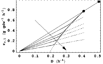
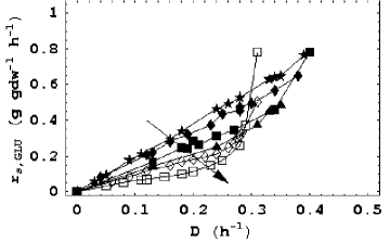
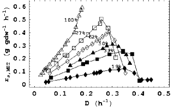
Figure 16: Near the transition dilution rate, the specific substrate uptake rates are independent of the feed composition. Upper panel: Model simulations. The arrows point in the direction of increasing $S_{2}$ in the feed. The full lines show the specific uptake rates predicted by numerical simulations of the model. The dashed lines show the specific uptake rates predicted by eqs. (51) and (57)–(58). Lower panel: Specific uptake rates of glucose and methanol during mixed-substrate growth of H. polymorpha (Egli et al., 1986, Figs. 4–5).

When $s_{2}\gg K_{s,2}$, eqs. (46) and (44) yield

$$x_{2} =\frac{r_{s,2}}{k_{x,2}}\approx\frac{V_{s,2}e_{2}}{k_{x,2}},$$

$$e_{2} =\frac{V_{e,2}}{D+k_{e,2}}-\frac{\bar{K}_{e,2}}{\sigma_{2}}\approx\frac{\bar{K}_{e,2}}{D+k_{e,2}}\left(D_{t,2}-D\right),$$ (56)

where the second relation was obtained by appealing to the approximations, $\sigma_{2},\sigma_{f,2}\approx 1$. Evidently,

$$r_{s,2}\approx V_{s,2}e_{2}$$ (57)

is a function of $D$. Since $Y_{1}r_{s,1}+Y_{2}r_{s,2}=D$, we conclude that

$$r_{s,1}=\frac{D-Y_{2}r_{s,2}}{Y_{1}},$$ (58)

and

$$x_{1} =\frac{r_{s,1}}{k_{x,1}},e_{1}=\frac{V_{e,1}}{D+k_{e,1}}\frac{x_{1}}{K_{e,1}+x_{1}},$$ (59)

are also functions of $D$.

Table 2: Parameter values used to simulate the growth of H. polymorpha on mixtures of glucose ($S_{1}$) and methanol ($S_{2}$). The yields are based on experimental measurements (Egli et al, 1986). The remaining parameters, which have not been measured experimentally, are based on order-of-magnitude estimates obtained from well-characterized systems, such as the lac operon (Shoemaker et al, 2003, Appendix A)

$i$	$Y_{i}$	$V_{s,i}$ (h-1)	$K_{s,i}$ (g L-1)	$k_{x,i}$ (h-1)	$V_{e,i}$ (h-1)	$K_{e,i}$	$k_{e,i}$ (h-1)
1	0.55	$10^{3}$	$10^{-2}$	$10^{3}$	$9\times 10^{-4}$	$7\times 10^{-4}$	0.05
2	0.38	$10^{3}$	$10^{-2}$	$10^{3}$	$3\times 10^{-4}$	$6\times 10^{-4}$	0.05

Since $r_{s,1}$ and $r_{s,2}$ are completely determined by $D$, the curves representing the specific substrate uptake rates at various feed compositions must collapse into a single curve. This conclusion is consistent with the data for growth of H. polymorpha on glucose + methanol (Figs. 16c,d). Indeed, simulations of the model, performed with the parameter values in Table 2, are in good agreement with the data, with the exception of two minor discrepancies (Figs. 16a,b). The specific uptake rates of glucose corresponding to 77%, and 62% methanol in the feed are discrepant for $D\gtrsim 0.25$ h^-1 (curves labeled $\square$ and $\lozenge$ in Fig. 16c). Likewise, the single-substrate specific uptake rate of methanol deviates from the model prediction when $D\gtrsim 0.15$ h^-1 (curve labeled $\triangle$ in Fig. 16d). Under these exceptional conditions, the residual methanol concentrations are so high that toxic effects arise, thus reducing the yields on glucose and methanol. The observed specific uptake rates are therefore higher than the predicted rates.

Eqs. (56)–(57) imply that at sufficiently high dilution rates, $e_{2}$ and $r_{s,2}$ decrease with $D$ until they become zero at $D=D_{t,2}$ (Fig. 17b). Consequently, $r_{s,1}$ and $e_{1}$ increase with $D$ to ensure that the total specific growth rate remains equal to $D$ (Fig. 17a). Both conclusions are consistent with the data for growth of H. polymorpha on glucose + methanol. The activities of the glucose enzymes, hexokinase and 6-phosphogluconate dehydrogenase, increase with $D$ (Fig. 17c), while the activity of the methanol enzyme, formaldehyde dehydrogenase, decreases with $D$ (Fig. 17d).

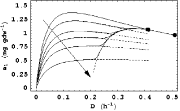
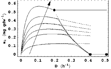
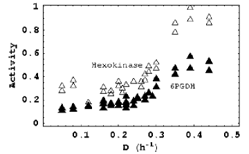
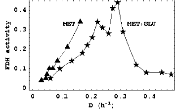
Figure 17: Variation of the peripheral enzyme levels for glucose and methanol. Upper panel: Model simulations. The arrows point in the direction of increasing $S_{2}$ in the feed. The full lines show the specific uptake rates predicted by numerical simulations of the model. The dashed lines show the enzyme levels predicted by eqs. (53) and (56), (59). Lower panel: Activities of (c) the glucose enzymes, hexokinase and 6-phoshogluconate dehydrogenase (6PGDH), and (d) the methanol enzyme, formaldehyde dehydrogenase, during mixed-substrate growth of H. polymorpha on 3 g L^-1 glucose and 2 g L^-1 methanol (Egli et al., 1982a, Fig. 4).

Since $r_{s,1}$ and $e_{1}$ are functions of $D$, so is

$$\sigma_{1}=\frac{r_{s,1}}{V_{s,1}e_{1}}.$$ (60)

In fact, the only variables that depend on the feed concentrations are the cell density and the concentration of $S_{2}$. To see this, it suffices to observe that eq. (43) yields

$$c =\frac{D(s_{f,1}-s_{1})}{r_{s,1}}\approx\left(\frac{D}{r_{s,1}}\right)s_{f,1},$$ (61)

$$s_{f,2}-s_{2} =\frac{r_{s,2}c}{D}\approx\left(\frac{r_{s,2}}{r_{s,1}}\right)s_{f,1},$$ (62)

where the terms in parentheses are functions of $D$. As expected, $c$ increases linearly with $s_{f,1}$ because growth is limited by $S_{1}$ only. Fig. 18 shows that numerical simulations of the model with the parameter values in Table 2 are in good agreement with the data for growth of H. polymorpha on glucose + methanol (Fig. 4).

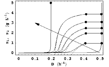
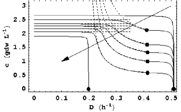
Figure 18: The model simulations are in good agreement with the data for growth of H. polymorpha on glucose + methanol shown in Fig. 4. The arrows point in the direction of increasing $S_{2}$ in the feed. The full lines show the substrate concentrations and cell density predicted by numerical simulations of the model. The dashed lines show the substrate concentrations and cell density predicted by eqs. (50), (54) and (60)–(62).

The patched limiting solutions approximate the exact solution

Taken together, the two approximate solutions corresponding to low and high dilution rates coincide with the (exact) numerical solution at all dilution rates, except in a small neighborhood of the dilution rate at which the two approximate solutions intersect (compare the dashed and full lines in Figs. 16–18). This remarkable agreement between the approximate and exact solution obtains because as $D$ increases, $s_{2}$ changes from subsaturating to saturating levels so rapidly that the change is, for all practical purposes, discontinuous. The switching dilution rate, $D_{s,2}$, provides a good approximation to the dilution rate at which this near-discontinuous change occurs. The model therefore provides explicit formulas that approximate the specific uptake rates, substrate concentrations, cell density, and enzyme levels at all dilution rates and saturating feed concentrations. The approximate solutions corresponding to low and high dilution rates are valid for $D<D_{s,2}$ and $D>D_{s,2}$, respectively.

Egli’s transition dilution rate differs from our transition dilution rate

There is an important difference between the transition dilution rates defined by Egli and us. In our model, $D_{t,2}$ is the dilution rate at which $e_{2}$, the activity of methanol enzymes becomes zero. This transition dilution rate, defined by eq. (42), increases with the feed concentration of methanol. However, at the saturating feed concentrations used in the experiments, it is essentially independent of the feed concentration. On the other hand, Egli defined the transition dilution rate empirically as the dilution rate at which the residual methanol concentration achieved a sufficiently high level (e.g., half the feed concentration of methanol). The mathematical correlate of this empirically defined transition dilution rate is the switching dilution rate, $D_{s,2}$ (at which $s_{2}$ switches from subsaturating to saturating levels). Consistent with Egli’s observations, $D_{s,2}$ decreases with the fraction of methanol in the feed. Indeed, (55) yields

$$\beta_{2}=Y_{2}V_{s,2}\bar{K}_{e,2}\frac{D_{t,2}-D_{s,2}}{D_{s,2}(D_{s,2}+k_{e,2})},$$

where $D_{t,2}$ is essentially constant at saturating feed concentrations. It follows that $D_{s,2}$ is a decreasing function of $\beta_{2}$, and, hence, $\psi_{2}$. Moreover, in the limiting cases of feeds consisting of almost pure methanol ($\beta_{2}\approx 1$) and pure glucose ($\beta_{2}\approx 0$), the switching dilution rate, $D_{s,2}$, tends to $D_{c,2}$ and $D_{t,2}$, respectively.

4 Discussion

We have shown above that a simple model accounting for only induction and growth captures the experimental data under a wide variety of conditions. This does not prove that the model is correct unless the underlying mechanism is consistent with experiments. Now, the model is based on following 3 assumptions. (a) The yield of biomass on a substrate is constant. (b) The induction rate follows hyperbolic kinetics, and regulatory mechanisms have a negligible effect on the induction rate. (c) Each substrate is transported by a unique system of lumped peripheral enzymes. In what follows, we discuss the validity of these assumptions.

4.1 Constant yields

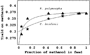
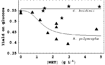
Figure 19: Yields on the substrates during growth of H. polymorpha and C. boidinii on glucose + methanol. (a) The yield on methanol is nearly constant at almost all feed concentrations (Egli et al., 1982b, Fig. 4). The dilution rate is fixed at $\sim$0.15 h^-1. (b) In H. polymorpha, the yield on glucose decreases $\sim$20% in the presence of high methanol concentrations (Egli et al., 1982a, Fig. 3).

Both direct and indirect evidence show that in many cases, the yield is, for the most part, constant.

Indirect evidence is obtained from experiments in which the specific growth and substrate uptake rates were measured during mixed-substrate growth at various dilution rates and feed concentrations. Given these rates, eq. (12) can be satisfied by infinitely many $Y_{1}$ and $Y_{2}$. It is therefore striking that in all these experiments, (12) is satisfied by the single-substrate yields on the two substrates. These include growth of E. coli on various sugars (Lendenmann et al., 1996; Smith and Atkinson, 1980), organic acids (Narang et al., 1997), glucose + 3-phenylpropionic acid (Kovarova et al., 1997); growth of Chelabacter heintzii on glucose + nitrilotriacetic acid (Bally et al., 1994); and growth of methylotrophic yeasts on methanol + glucose (Fig. 13c) and methanol + sorbitol (Eggeling and Sahm, 1981).

Direct evidence is obtained from experiments in which at least one of the yields was measured by using radioactively labeled substrates (Fig. 19). These measurements show that the yield on a substrate remains essentially equal to the single-substrate yield, except when toxic effects arise, or the fraction of the substrate in the feed is below $\sim$10%  (Rudolph and Grady, 2001).

4.2 Induction kinetics

The induction kinetics and regulatory mechanisms can influence the behavior of the model. Specifically, if the induction kinetics are sigmoidal, multiple stable steady states arise, resulting in the manifestation of the maintenance or pre-induction effect (Narang, 1998a; Narang and Pilyugin, 2007b). Likewise, introduction of regulatory effects in the model will alter its quantitative predictions (although the analysis of the data for the lac operon shows that regulatory effects play a minor role). However, the essential property of the model, namely, the competitive (Lotka-Volterra) interaction between the enzymes, is unaffected by these changes — the model still predicts the existence of extinction and coexistence steady states obtained with the minimal model (see Section 4.1 of Narang and Pilyugin, 2007a).

4.3 Transport kinetics

Many substrates are imported into the cell by two (or more) transport systems (Ferenci, 1996, Table 1). In general, these transport systems dominate substrate import at different substrate concentrations. For instance, galactose is transported by the low-affinity galactose permease under substrate-excess conditions, and the high-affinity methylgalactosidase system under substrate-limiting conditions (Weickert and Adhya, 1993). If these transport systems dominate in distinct regimes of the dilution rate, they are unlikely to have a significant effect on the model. However, if the two regimes overlap, it is difficult to predict the outcome without analyzing a suitably extended model. This will be the focus of future work.

Lumping of peripheral enzymes has a profound effect if the inducer is synthesized and consumed by coordinately expressed enzymes. Following Savageau, we illustrate this point by appealing to the lac operon (Savageau, 2001, Fig. 10). It turns out that the concentration of the inducer, allolactose, is completely determined by the concentration of intracellular lactose. Moreover, the dynamics of intracellular lactose, denoted $x$, are given by the equation

$$\frac{dx}{dt}=V_{s}e_{p}\frac{s}{K_{s}+s}-k_{x}e_{b}x-r_{g}x,$$

where $s$ denotes extracellular lactose, $e_{p}$ denotes permease, and $e_{b}$ denotes $\beta$-galactosidase. Since permease and $\beta$-galactosidase are encoded by the same operon, intuition suggests that they must be coordinately expressed, i.e., $e_{p}=e_{b}$. It follows that the quasisteady state concentration of intracellular lactose, $x\approx(V_{s}/k_{x})s/(K_{s}+s)$, is independent of the enzyme level. Thus, positive feedback, a key component of the model disappears if the inducer (or its precursor) is synthesized by coordinately expressed enzymes. Under this condition, the positive feedback generated by one of the enzymes (e.g., permease) is neutralized by the other enzyme (e.g., $\beta$-galactosidase).

The relative rates of permease and $\beta$-galactosidase expression are not known, but there is good evidence that galactosidase and transacetylase are not expressed coordinately (reviewed in Adhya, 2003). Indeed, Ullmann and coworkers have shown that the higher the protein synthesis rate, the higher the relative rate of transacetylase synthesis (Danchin et al., 1981). Furthermore, this uncoupling occurs at the level of transcription, and involves the transcription termination factor, Rho (Guidi-Rontani et al., 1984). It seems likely that permease and $\beta$-galactosidase are also uncoupled, but this remains a hypothesis until direct evidence is obtained.

5 Conclusions

We formulated a minimal model of mixed-substrate growth that accounts for only induction and growth (but no regulation), the two processes that occur in all microbes including bacteria and yeasts.

1. Quantitative analysis of the data for both bacteria and yeasts shows that the decline of the enzyme activities in constitutive and wild-type cells, typically attributed to specific regulatory mechanisms, is almost entirely due to dilution.

2. We analyzed the model by constructing the bifurcation diagrams for both batch and continuous cultures.

   1. The bifurcation diagram for batch cultures describes the substrate consumption patterns at any given initial substrate concentrations. It shows that: (i) When the initial concentrations of one or more substrates are sufficiently small, threshold effects arise because the enzymes cannot be induced. (ii) Even if the initial concentrations of both substrates are at supra-threshold levels, induction of the enzymes for one of the substrates may not occur because of dilution. Thus, diauxic growth is feasible even if there are no regulatory mechanisms. (c) The substrate consumption pattern can be switched from sequential to simultaneous (or vice versa) by altering the initial substrate concentrations. All these conclusions are consistent with the data in the literature.

   2. The bifurcation diagram for continuous cultures, which describes the substrate consumption patterns at any given dilution rate and feed concentrations, is formally identical to the bifurcation diagram for batch cultures. This gives a precise mathematical basis for the well-known empirical correlation between the growth patterns in batch and continuous cultures. Specifically, substrates that are simultaneously consumed in substrate-excess batch cultures are consumed simultaneously in continuous cultures at all dilution rates up to washout. However, substrates that are sequentially consumed in substrate-excess batch cultures are consumed simultaneously in continuous cultures only if the dilution rate is sufficiently small — at large dilution rates, only the preferred substrate is consumed. This switch occurs precisely at the so-called transition dilution rate because synthesis of the secondary substrate enzymes is abolished by dilution. The transition dilution rate is significantly higher the maximum growth rate on the secondary substrate. This “enhanced growth effect” occurs because the enzyme levels are positive at the critical dilution rate of the secondary substrate — they become vanishingly small only if the cells are subjected to even higher dilution rates.

3. At the saturating feed concentrations typically used in experiments, the physiological steady states are completely determined by only two independent parameters, the dilution rate and the mass fraction of the substrate in the feed. We derived analytical expressions for the steady state values of the substrates, cell density, and enzymes that provide good fits to the extensive data for the growth of methylotrophic yeasts on glucose and methanol.

Appendix A Bifurcation diagram for batch cultures

A.1 Conditions for existence and stability of the steady states

The steady states that can be attained during the first few hours of batch growth are given by the equations

$$0=\frac{de_{1}}{dt} =V_{e,1}\frac{e_{1}\sigma_{0,1}}{\bar{K}_{e,1}+e_{1}\sigma_{0,1}}-\left(Y_{1}V_{s,1}e_{1}\sigma_{0,1}+Y_{2}V_{s,2}e_{2}\sigma_{0,2}+k_{e,1}\right)e_{1},$$ (63)

$$0=\frac{de_{2}}{dt} =V_{e,2}\frac{e_{2}\sigma_{0,2}}{\bar{K}_{e,2}+e_{2}\sigma_{0,2}}-\left(Y_{1}V_{s,1}e_{1}\sigma_{0,1}+Y_{2}V_{s,2}e_{2}\sigma_{0,2}+k_{e,2}\right)e_{2}.$$ (64)

The Jacobian has the form

$$J(e_{1},e_{2})=\left[\begin{array}[]{cc}J_{11}&-Y_{2}V_{s,2}e_{1}\sigma_{0,2}\\ -Y_{1}V_{s,1}e_{2}\sigma_{0,1}&J_{22}\end{array}\right],$$ (65)

where

$$J_{11} \equiv V_{e,1}\frac{\bar{K}_{e,1}\sigma_{0,1}}{\left(\bar{K}_{e,1}+e_{1}\sigma_{0,1}\right)^{2}}-2Y_{1}V_{s,1}e_{1}\sigma_{0,1}-Y_{2}V_{s,2}e_{2}\sigma_{0,2}-k_{e,1},$$ (66)

$$J_{22} \equiv V_{e,2}\frac{\bar{K}_{e,2}\sigma_{0,2}}{\left(\bar{K}_{e,2}+e_{2}\sigma_{0,2}\right)^{2}}-Y_{1}V_{s,1}e_{1}\sigma_{0,1}-2Y_{2}V_{s,2}e_{2}\sigma_{0,2}-k_{e,2}.$$ (67)

In what follows, we derive the existence and stability conditions for each of the 4 steady states.

1. $E_{00}$ ($e_{1}=0,e_{2}=0$): It is evident from (63)–(64) that this steady always exists. Since

   $$J(E_{00})=\left[\begin{array}[]{cc}\frac{V_{e,1}\sigma_{0,1}}{\bar{K}_{e,1}}-k_{e,1}&0\\ 0&\frac{V_{e,2}\sigma_{0,2}}{\bar{K}_{e,2}}-k_{e,2}\end{array}\right],$$

   $E_{00}$ is stable if and only if

   $$r_{g,i}^{*}\equiv\frac{V_{e,i}\sigma_{0,i}}{\bar{K}_{e,i}}-k_{e,i}<0 \Leftrightarrow\sigma_{0,i}<\sigma_{i}^{*}\equiv\frac{k_{e,i}}{V_{e,i}/\bar{K}_{e,i}}$$

   for $i=1,2$.

2. $E_{10}$ ($e_{1}>0,e_{2}=0$): This steady state exists if and only if the equation

   $$V_{e,1}\frac{\sigma_{0,1}}{\bar{K}_{e,1}+e_{1}\sigma_{0,1}}=Y_{1}V_{s,1}e_{1}\sigma_{0,1}+k_{e,1}$$ (68)

   has a positive solution, $e_{1}>0$. Such a solution exists precisely when

   $$r_{g,1}^{*}>0\Leftrightarrow\sigma_{0,1}>\sigma_{1}^{*},$$

   in which case

   $$\left.e_{1}\right|_{E_{10}} =\frac{-\left(\bar{K}_{e,1}+\frac{k_{e,1}}{Y_{1}V_{s,1}}\right)+\sqrt{\left(\bar{K}_{e,1}+\frac{k_{e,1}}{Y_{1}V_{s,1}}\right)^{2}+\frac{4\bar{K}_{e,1}r_{g,1}^{*}}{Y_{1}V_{s,1}}}}{2\sigma_{0,1}},$$

   $$r_{g,1} =Y_{1}V_{s,1}\frac{-\left(\bar{K}_{e,1}+\frac{k_{e,1}}{Y_{1}V_{s,1}}\right)+\sqrt{\left(\bar{K}_{e,1}+\frac{k_{e,1}}{Y_{1}V_{s,1}}\right)^{2}+\frac{4\bar{K}_{e,1}r_{g,1}^{*}}{Y_{1}V_{s,1}}}}{2},$$ (69)

   where $r_{g,1}\equiv\left.Y_{1}V_{s,1}e_{1}\sigma_{0,1}\right|_{E_{10}}$ is the exponential growth rate at $E_{10}$.
   To determine the stability conditions, observe that

   $$J(E_{10})=\left[\begin{array}[]{cc}J_{11}&-Y_{2}V_{s,2}e_{1}\sigma_{0,2}\\ 0&J_{22}\end{array}\right],$$

   where

   $$J_{11} =V_{e,1}\frac{\bar{K}_{e,1}\sigma_{0,1}}{\left(\bar{K}_{e,1}+e_{1}\sigma_{0,1}\right)^{2}}-2Y_{1}V_{s,1}e_{1}\sigma_{0,1}-k_{e,1},$$

   $$J_{22} =V_{e,2}\frac{\sigma_{0,2}}{\bar{K}_{e,2}}-Y_{1}V_{s,1}e_{1}\sigma_{0,1}-k_{e,2}.$$

   Now, $J_{11}$ is always negative because (68) implies that at $E_{10}$,

   $$V_{e,1}\frac{\bar{K}_{e,1}\sigma_{0,1}}{\left(\bar{K}_{e,1}+e_{1}\sigma_{0,1}\right)^{2}}=\frac{\bar{K}_{e,1}}{\bar{K}_{e,1}+e_{1}\sigma_{0,1}}\left(Y_{1}V_{s,1}e_{1}\sigma_{0,1}+k_{e,1}\right),$$

   so that

   $$J_{11}=-\left(Y_{1}V_{s,1}e_{1}\sigma_{0,1}+k_{e,1}\right)\frac{e_{1}\sigma_{0,1}}{\bar{K}_{e,1}+e_{1}\sigma_{0,1}}-Y_{1}V_{s,1}e_{1}\sigma_{0,1}<0.$$

   Hence, $E_{10}$ is stable if and only if

   $$J_{22}<0 \Leftrightarrow V_{e,2}\frac{\sigma_{0,2}}{\bar{K}_{e,2}}<\left.Y_{1}V_{s,1}e_{1}\sigma_{0,1}\right|_{E_{10}}+k_{e,2},$$

   $$\Leftrightarrow r_{g,2}^{*}<r_{g,1}.$$

3. $E_{01}$ ($e_{1}=0,e_{2}>0$): Arguments similar to those used above for $E_{10}$ show that $E_{01}$ exists if and only if

   $$r_{g,2}^{*}>0\Leftrightarrow\sigma_{0,2}>\sigma_{2}^{*},$$

   in which case

   $$\left.e_{2}\right|_{E_{01}} =\frac{-\left(\bar{K}_{e,2}+\frac{k_{e,2}}{Y_{2}V_{s,2}}\right)+\sqrt{\left(\bar{K}_{e,2}+\frac{k_{e,2}}{Y_{2}V_{s,2}}\right)^{2}+\frac{4\bar{K}_{e,2}r_{g,2}^{*}}{Y_{2}V_{s,2}}}}{2\sigma_{0,2}},$$

   $$r_{g,2}^{\textnormal{max}} =Y_{2}V_{s,2}\frac{-\left(\bar{K}_{e,2}+\frac{k_{e,2}}{Y_{2}V_{s,2}}\right)+\sqrt{\left(\bar{K}_{e,2}+\frac{k_{e,2}}{Y_{2}V_{s,2}}\right)^{2}+\frac{4\bar{K}_{e,2}r_{g,2}^{*}}{Y_{2}V_{s,2}}}}{2},$$ (70)

   where $r_{g,2}\equiv\left.Y_{2}V_{s,2}e_{2}\sigma_{0,2}\right|_{E_{01}}$ is the exponential growth rate at $E_{01}$.

4. $E_{11}$ ($e_{1}>0,e_{2}>0$): This steady state exists if and only if the equations

   $$0 =V_{e,1}\frac{\sigma_{0,1}}{\bar{K}_{e,1}+e_{1}\sigma_{0,1}}-\left(Y_{1}V_{s,1}e_{1}\sigma_{0,1}+Y_{2}V_{s,2}e_{2}\sigma_{0,2}+k_{e,1}\right),$$ (71)

   $$0 =V_{e,2}\frac{\sigma_{0,2}}{\bar{K}_{e,2}+e_{2}\sigma_{0,2}}-\left(Y_{1}V_{s,1}e_{1}\sigma_{0,1}+Y_{2}V_{s,2}e_{2}\sigma_{0,2}+k_{e,2}\right),$$ (72)

   have positive solutions, $e_{1},e_{2}>0$. The conditions for such solutions can be determined by eliminating one of the variables, $e_{1},e_{2}$, from the above equations. To this end, observe that eqs. (71)–(72) imply the relation

   $$V_{e,1}\frac{\sigma_{0,1}}{\bar{K}_{e,1}+e_{1}\sigma_{0,1}}-k_{e,1}=V_{e,2}\frac{\sigma_{0,2}}{\bar{K}_{e,2}+e_{2}\sigma_{0,2}}-k_{e,2}.$$ (73)

   Hence, we can eliminate $e_{2}$ from (71)–(72) by solving (73) for $e_{2}$, and substituting it in (71) to obtain the equation

   $$V_{e,1}\frac{\sigma_{0,1}}{\bar{K}_{e,1}+e_{1}\sigma_{0,1}}-k_{e,1} =Y_{1}V_{s,1}e_{1}\sigma_{0,1}+Y_{2}V_{s,2}\frac{V_{e,2}\sigma_{0,2}}{V_{e,1}\frac{\sigma_{0,1}}{\bar{K}_{e,1}+\sigma_{0,1}}-k_{e,1}+k_{e,2}}$$

   $$\quad\quad\quad-Y_{2}V_{s,2}\bar{K}_{e,2},$$

   which has a (unique) positive solution, $e_{1}>0$, if and only if

   $$\frac{V_{e,1}\sigma_{0,1}}{\bar{K}_{e,1}}-k_{e,1}>Y_{2}V_{s,2}\frac{V_{e,2}\sigma_{0,1}}{\left(\frac{V_{e,1}\sigma_{0,1}}{\bar{K}_{e,1}}-k_{e,1}\right)+k_{e,2}}-Y_{2}V_{s,2}\bar{K}_{e,2}.$$

   One can check that this is equivalent to the condition

   $$r_{g,1}^{*}\equiv\frac{V_{e,1}\sigma_{0,1}}{\bar{K}_{e,1}}-k_{e,1}>\left.Y_{2}V_{s,2}e_{2}\sigma_{0,2}\right|_{E_{01}}\equiv r_{g,2},$$

   i.e., $E_{10}$ is unstable.
   Similarly, eliminating $e_{1}$ from (71)-(72) yields

   $$V_{e,2}\frac{\sigma_{0,2}}{\bar{K}_{e,1}+e_{2}\sigma_{0,2}}-k_{e,2} =Y_{2}V_{s,2}e_{2}\sigma_{0,2}+Y_{1}V_{s,1}\frac{V_{e,1}\sigma_{0,1}}{V_{e,2}\frac{\sigma_{0,2}}{\bar{K}_{e,2}+\sigma_{0,2}}-k_{e,2}+k_{e,1}}$$

   $$\quad\quad\quad-Y_{1}V_{s,1}\bar{K}_{e,1},$$

   which has a positive solution, $e_{2}>0$, if and only if $E_{10}$ is unstable. We conclude that $E_{11}$ exists and is unique if and only if both $E_{10}$ and $E_{01}$ (exist and) are unstable.
   To determine the stability condition, observe that (71) implies

   $$V_{e,1}\frac{\bar{K}_{e,1}\sigma_{0,1}}{\left(\bar{K}_{e,1}+e_{1}\sigma_{0,1}\right)^{2}}=\left(Y_{1}V_{s,1}e_{1}\sigma_{0,1}+Y_{2}V_{s,2}e_{2}\sigma_{0,2}+k_{e,1}\right)\frac{\bar{K}_{e,1}}{\bar{K}_{e,1}+e_{1}\sigma_{0,1}}.$$

   Hence,

   $$J_{11} =\left(Y_{1}V_{s,1}e_{1}\sigma_{0,1}+Y_{2}V_{s,2}e_{2}\sigma_{0,2}+k_{e,1}\right)\frac{\bar{K}_{e,1}}{\bar{K}_{e,1}+e_{1}\sigma_{0,1}}$$

   $$\quad\quad\quad-2Y_{1}V_{s,1}e_{1}\sigma_{0,1}-Y_{2}V_{s,2}e_{2}\sigma_{0,2}-k_{e,2},$$

   $$=-\left(Y_{1}V_{s,1}e_{1}\sigma_{0,1}+Y_{2}V_{s,2}e_{2}\sigma_{0,2}+k_{e,1}\right)\frac{e_{1}\sigma_{0,1}}{\bar{K}_{e,1}+e_{1}\sigma_{0,1}}-Y_{1}V_{s,1}e_{1}\sigma_{0,1},$$

   and similarly,

   $$J_{22}=-\left(Y_{1}V_{s,1}e_{1}\sigma_{0,1}+Y_{2}V_{s,2}e_{2}\sigma_{0,2}+k_{e,1}\right)\frac{e_{2}\sigma_{0,2}}{\bar{K}_{e,2}+e_{2}\sigma_{0,2}}-Y_{2}V_{s,2}e_{2}\sigma_{0,2}.$$

   It follows immediately that $\textnormal{tr}\,J<0$ and $\det J>0$. Hence, $E_{11}$ is stable whenever it exists.

A.2 Relative magnitudes of $r_{g,i}$ and $r_{g,i}^{*}$

The exponential growth rate on $S_{i}$, $r_{g,i}(\sigma_{0,i})$, is always less than $r_{g,i}^{*}(\sigma_{0,i})$, the specific growth rate at which $E_{i}$ becomes extinct. To see this, observe that (69)–(70) can be rewritten as

$$r_{g,i}^{*}=\left(1+\frac{k_{e,i}}{Y_{i}V_{s,i}\bar{K}_{e,i}}\right)r_{g,i}+\left(\frac{1}{Y_{i}V_{s,i}\bar{K}_{e,i}}\right)r_{g,i}^{2},$$ (74)

which implies that

$$r_{g,i}\leq r_{g,i}^{*},$$

with equality being attained when $\sigma_{i}=\sigma_{i}^{*}$, in which case, $r_{g,i}=r_{g,i}^{*}=0$.

A.3 Disposition of the bifurcation curves

The lower (blue) bifurcation curve in Fig. 9 is defined by the condition

$$r_{g,1} =r_{g,2}^{*}.$$ (75)

Since

$$r_{g,1}^{*}=\left(1+\frac{k_{e,1}}{Y_{1}V_{s,1}\bar{K}_{e,1}}\right)r_{g,1}+\left(\frac{1}{Y_{1}V_{s,1}\bar{K}_{e,1}}\right)r_{g,1}^{2},$$ (76)

the bifurcation curve defined by (75) satisfies the equation

$$r_{g,1}^{*}=\left(1+\frac{k_{e,1}}{Y_{1}V_{s,1}\bar{K}_{e,1}}\right)r_{g,2}^{*}+\frac{1}{Y_{1}V_{s,1}\bar{K}_{e,1}}\left(r_{g,2}^{*}\right)^{2},$$

obtained from (76) by replacing $r_{g,1}$ with $r_{g,2}^{*}$. Substituting the definition of $r_{g,i}^{*}$ into the above equation yields

$$\frac{V_{e,1}}{\bar{K}_{e,1}}\left(\sigma_{0,1}-\sigma_{1}^{*}\right) =\left(1+\frac{k_{e,1}}{Y_{1}V_{s,1}\bar{K}_{e,1}}\right)\left[\frac{V_{e,2}}{\bar{K}_{e,2}}\left(\sigma_{0,2}-\sigma_{2}^{*}\right)\right]$$

$$\qquad+\frac{1}{Y_{1}V_{s,1}\bar{K}_{e,1}}\left[\frac{V_{e,2}}{\bar{K}_{e,2}}\left(\sigma_{0,2}-\sigma_{2}^{*}\right)\right]^{2},$$

which defines an increasing curve on the $\sigma_{0,1},\sigma_{0,2}$-plane passing through the point $\left(\sigma_{1}^{*},\sigma_{2}^{*}\right)$. Moreover, since the points on this curve satisfy the relation

$$\frac{V_{e,1}}{\bar{K}_{e,1}}\left(\sigma_{0,1}-\sigma_{1}^{*}\right)>\frac{V_{e,2}}{\bar{K}_{e,2}}\left(\sigma_{0,2}-\sigma_{2}^{*}\right),$$

they never go above the line

$$\frac{V_{e,1}}{\bar{K}_{e,1}}\left(\sigma_{0,1}-\sigma_{1}^{*}\right)=\frac{V_{e,2}}{\bar{K}_{e,2}}\left(\sigma_{0,2}-\sigma_{2}^{*}\right).$$ (77)

A similar argument shows that the upper (red) bifurcation curve in Fig. 9, which is defined by the equation

$$r_{g,2}=r_{g,1}^{*},$$ (78)

satisfies the relation

$$\frac{V_{e,2}}{\bar{K}_{e,2}}\left(\sigma_{0,2}-\sigma_{2}^{*}\right) =\left(1+\frac{k_{e,2}}{Y_{2}V_{s,2}\bar{K}_{e,2}}\right)\left[\frac{V_{e,1}}{\bar{K}_{e,1}}\left(\sigma_{0,2}-\sigma_{1}^{*}\right)\right]$$

$$\qquad+\frac{1}{Y_{2}V_{s,2}\bar{K}_{e,12}}\left[\frac{V_{e,1}}{\bar{K}_{e,1}}\left(\sigma_{0,1}-\sigma_{1}^{*}\right)\right]^{2}.$$

This relation also defines an increasing curve passing through $\left(\sigma_{1}^{*},\sigma_{2}^{*}\right)$, but the curve never goes below the line defined by (77) because

$$\frac{V_{e,2}}{\bar{K}_{e,2}}\left(\sigma_{0,2}-\sigma_{2}^{*}\right)>\frac{V_{e,1}}{\bar{K}_{e,1}}\left(\sigma_{0,1}-\sigma_{1}^{*}\right).$$

Hence, the curve defined by (78) always lies above the curve defined by (75).

Finally, we note that as the two bifurcation curves approach the point, $(\sigma_{1}^{*},\sigma_{2}^{*})$, they are approximated by the lines

$$\frac{V_{e,1}}{\bar{K}_{e,1}}\left(\sigma_{0,1}-\sigma_{1}^{*}\right) \approx\left(1+\frac{k_{e,1}}{Y_{1}V_{s,1}\bar{K}_{e,1}}\right)\left[\frac{V_{e,2}}{\bar{K}_{e,2}}\left(\sigma_{0,2}-\sigma_{2}^{*}\right)\right],$$

$$\frac{V_{e,2}}{\bar{K}_{e,2}}\left(\sigma_{0,2}-\sigma_{2}^{*}\right) \approx\left(1+\frac{k_{e,2}}{Y_{2}V_{s,2}\bar{K}_{e,2}}\right)\left[\frac{V_{e,1}}{\bar{K}_{e,1}}\left(\sigma_{0,1}-\sigma_{1}^{*}\right)\right],$$

which almost coincide with the line defined by (77) because $k_{e,i}\ll Y_{i}V_{s,i}\bar{K}_{e,i}$. Thus, for typical parameter values, the curves have the quasicusp-shaped geometry shown in Fig. 9.

Appendix B Bifurcation diagram for continuous cultures

The steady states of continuous cultures satisfy the equations

$$0=\frac{ds_{1}}{dt} =D\left(s_{f,1}-s_{1}\right)-r_{s,1}c,$$ (79)

$$0=\frac{ds_{2}}{dt} =D\left(s_{f,2}-s_{1}\right)-r_{s,2}c,$$ (80)

$$0=\frac{dc}{dt} =\left(r_{g}-D\right)c,$$ (81)

$$0=\frac{de_{1}}{dt} =R_{1}\equiv V_{e,1}\frac{e_{1}\sigma_{1}}{\bar{K}_{e,1}+e_{1}\sigma_{1}}-\left(r_{g}+k_{e,1}\right)e_{1},$$ (82)

$$0=\frac{de_{2}}{dt} =R_{2}\equiv V_{e,2}\frac{e_{2}\sigma_{2}}{\bar{K}_{e,2}+e_{2}\sigma_{2}}-\left(r_{g}+k_{e,2}\right)e_{2},$$ (83)

where $r_{g}=Y_{1}r_{s,1}+Y_{2}r_{s,2}$. The Jacobian is

$$J=\left[\begin{array}[]{ccccc}-D-c\frac{\partial r_{s,1}}{\partial s_{1}}&0&-r_{s,1}&-c\frac{\partial r_{s,1}}{\partial e_{1}}&0\\ 0&-D-c\frac{\partial r_{s,2}}{\partial s_{2}}&-r_{s,2}&0&-c\frac{\partial r_{s,2}}{\partial e2_{1}}\\ c\frac{\partial r_{g}}{\partial s_{1}}&c\frac{\partial r_{g}}{\partial s_{2}}&r_{g}-D&c\frac{\partial r_{g}}{\partial e_{1}}&c\frac{\partial r_{g}}{\partial e_{2}}\\ \frac{\partial R_{1}}{\partial s_{1}}&\frac{\partial R_{1}}{\partial s_{2}}&0&\frac{\partial R_{1}}{\partial e_{1}}&\frac{\partial R_{1}}{\partial e_{2}}\\ \frac{\partial R_{2}}{\partial s_{1}}&\frac{\partial R_{2}}{\partial s_{2}}&0&\frac{\partial R_{2}}{\partial e_{1}}&\frac{\partial R_{2}}{\partial e_{2}}\end{array}\right]$$ (84)

We begin by considering the washout steady states ($c=0$), since the existence and stability conditions for these steady states follow immediately from the foregoing analysis of batch cultures.

B.1 Existence and stability of washout steady states

At a washout steady state, $c=0,s_{1}=s_{f,1},s_{2}=s_{f,2}$. Such a steady state exists if and only if there exist $e_{1},e_{2}>0$ satisfying the equations

$$0=\frac{de_{1}}{dt} =V_{e,1}\frac{e_{1}\sigma_{f,1}}{\bar{K}_{e,1}+e_{1}\sigma_{f,1}}-\left(Y_{1}V_{s,1}e_{1}\sigma_{f,1}+Y_{2}V_{s,2}e_{2}\sigma_{f,2}+k_{e,1}\right)e_{1},$$

$$0=\frac{de_{2}}{dt} =V_{e,2}\frac{e_{2}\sigma_{f,2}}{\bar{K}_{e,2}+e_{2}\sigma_{f,2}}-\left(Y_{1}V_{s,1}e_{1}\sigma_{f,1}+Y_{2}V_{s,2}e_{2}\sigma_{f,2}+k_{e,2}\right)e_{2},$$

which are formally similar to eqs. (63)–(64), the only difference being that $\sigma_{0,i}$ is replaced by $\sigma_{f,i}$.

It follows from (84) that the Jacobian at a washout steady steady is

$$J=\left[\begin{array}[]{ccccc}-D&0&-r_{s,1}&0&0\\ 0&-D&-r_{s,2}&0&0\\ 0&0&r_{g}-D&0&0\\ \frac{\partial R_{1}}{\partial s_{1}}&\frac{\partial R_{1}}{\partial s_{2}}&0&\frac{\partial R_{1}}{\partial e_{1}}&\frac{\partial R_{1}}{\partial e_{2}}\\ \frac{\partial R_{2}}{\partial s_{1}}&\frac{\partial R_{2}}{\partial s_{2}}&0&\frac{\partial R_{2}}{\partial e_{1}}&\frac{\partial R_{2}}{\partial e_{2}}\end{array}\right].$$

Thus, a washout steady state is stable if and only if at this steady state, $r_{g}<D$, and the submatrix

$$R\equiv\left[\begin{array}[]{cc}\frac{\partial R_{1}}{\partial e_{1}}&\frac{\partial R_{1}}{\partial e_{2}}\\ \frac{\partial R_{2}}{\partial e_{1}}&\frac{\partial R_{2}}{\partial e_{2}}\end{array}\right]$$

has negative eigenvalues. This submatrix is formally similar to the matrix defined by eqs. (65)–(67), the only difference being that $\sigma_{0,i}$ is replaced by $\sigma_{f,i}$.

Given the above results, we expect the existence and stability conditions for the washout steady states, $E_{000}$, $E_{100}$, $E_{010}$, $E_{110}$, to be formally similar to the existence and stability conditions for the corresponding batch culture steady states, namely, $E_{00}$, $E_{10}$, $E_{01}$, and $E_{11}$. We show below that this is indeed the case.

1. $E_{000}$ ($e_{1}=0$, $e_{2}=0$, $c=0$): It is evident that this steady state always exists. Since $\left.r_{g}\right|_{E_{000}}=0<D$, $E_{000}$ is stable if and only if $R(E_{000})$ has negative eigenvalues. Since $R(E_{000})$ is formally similar to $J(E_{00})$, we conclude that $E_{000}$ is stable if and only if

   $$D_{t,i}\equiv\frac{V_{e,i}\sigma_{f,i}}{\bar{K}_{e,i}}-k_{e,i}<0\Leftrightarrow\sigma_{f,i}<\sigma_{i}^{*}\equiv\frac{k_{e,i}}{V_{e,i}/K_{e,i}}$$ (85)

   for $i=1,2$.

2. $E_{100}$ ($e_{1}>0$, $e_{2}=0$, $c=0$): This steady state exists if and only if

   $$V_{e,1}\frac{\sigma_{f,1}}{\bar{K}_{e,1}+e_{1}\sigma_{f,1}}=Y_{1}V_{s,1}e_{1}\sigma_{f,1}+k_{e,1}$$ (86)

   which is formally similar to eq. (68). It follows that $E_{100}$ exists if and only if

   $$D_{t,1}>0\Leftrightarrow\sigma_{f,1}>\sigma_{1}^{*},$$

   in which case

   $$\left.e_{1}\right|_{E_{100}} =\frac{-\left(\bar{K}_{e,1}+\frac{k_{e,1}}{Y_{1}V_{s,1}}\right)+\sqrt{\left(\bar{K}_{e,1}+\frac{k_{e,1}}{Y_{1}V_{s,1}}\right)^{2}+\frac{4K_{e,1}D_{t,1}}{Y_{1}V_{s,1}}}}{2\sigma_{f,1}},$$

   $$D_{c,1} =Y_{1}V_{s,1}\frac{-\left(\bar{K}_{e,1}+\frac{k_{e,1}}{Y_{1}V_{s,1}}\right)+\sqrt{\left(\bar{K}_{e,1}+\frac{k_{e,1}}{Y_{1}V_{s,1}}\right)^{2}+\frac{4K_{e,1}D_{t,1}}{Y_{1}V_{s,1}}}}{2},$$ (87)

   where $D_{c,1}\equiv\left.r_{g}\right|_{E_{100}}=\left.Y_{1}V_{s,1}e_{1}\sigma_{1}\right|_{E_{100}}$ is the critical dilution rate during single-substrate growth on $S_{1}$.
   $E_{100}$ is stable if and only if $D>D_{c,1}$ and $D_{t,2}<D_{c,1}$, where the latter relation ensures that the submatrix, $R(E_{100})$, which is formally similar to $J(E_{10})$, has negative eigenvalues. In the particular case of single-substrate growth on $S_{1}$, the second stability condition is always satisfied ($D_{t,2}=-k_{e,2}<0<D_{c,1}$), so that $E_{100}$ is stable whenever $D>D_{c,1}$.

3. $E_{010}$ ($e_{1}=0$, $e_{2}>0$, $c=0$): Arguments similar to those used above for $E_{100}$ show that $E_{010}$ exists if and only if

   $$D_{t,2}>0\Leftrightarrow\sigma_{f,2}>\sigma_{2}^{*},$$

   in which case

   $$\left.e_{2}\right|_{E_{010}} =\frac{-\left(\bar{K}_{e,2}+\frac{k_{e,2}}{Y_{2}V_{s,2}}\right)+\sqrt{\left(\bar{K}_{e,2}+\frac{k_{e,2}}{Y_{2}V_{s,2}}\right)^{2}+\frac{4K_{e,2}D_{t,2}}{Y_{2}V_{s,2}}}}{2\sigma_{f,2}},$$

   $$D_{c,2} =Y_{2}V_{s,2}\frac{-\left(\bar{K}_{e,2}+\frac{k_{e,2}}{Y_{2}V_{s,2}}\right)+\sqrt{\left(\bar{K}_{e,2}+\frac{k_{e,2}}{Y_{2}V_{s,2}}\right)^{2}+\frac{4K_{e,2}D_{t,2}}{Y_{2}V_{s,2}}}}{2},$$ (88)

   where $D_{c,2}\equiv\left.r_{g}\right|_{E_{010}}=\left.Y_{2}V_{s,2}e_{2}\sigma_{2}\right|_{E_{010}}$ is the critical dilution rate during single-substrate growth on $S_{2}$. It is stable if and only if $D>D_{c,2}$ and $D_{t,1}<D_{c,2}$.

4. $E_{110}$ ($e_{1}=0$, $e_{2}>0$, $c>0$): This steady state exists if and only if the equations

   $$0 =V_{e,1}\frac{\sigma_{f,1}}{\bar{K}_{e,1}+e_{1}\sigma_{f,1}}-\left(Y_{1}V_{s,1}e_{1}\sigma_{f,1}+Y_{2}V_{s,2}e_{2}\sigma_{f,2}+k_{e,1}\right),$$ (89)

   $$0 =V_{e,2}\frac{\sigma_{f,2}}{\bar{K}_{e,2}+e_{2}\sigma_{f,2}}-\left(Y_{1}V_{s,1}e_{1}\sigma_{f,1}+Y_{2}V_{s,2}e_{2}\sigma_{f,2}+k_{e,2}\right),$$ (90)

   have positive solutions. These equations are formally similar to eqs. (71)–(72). Hence, $E_{110}$ exists and is unique if and only if

   $$0<D_{t,2}<D_{c,1},\;0<D_{t,1}<D_{c,2}.$$

   Since $R(E_{110})$ is formally similar to $J(E_{11})$, the eigenvalues of $R(E_{110})$ are always negative. It follows that $E_{110}$ is stable if and only if

   $$D>D_{c}\equiv\left.r_{g}\right|_{E_{110}}=\left.Y_{1}V_{s,1}e_{1}\sigma_{1}+Y_{2}V_{s,2}e_{2}\sigma_{2}\right|_{E_{110}}.$$

   We cannot solve explicitly for $D_{c}$, but its properties can be inferred from an implicit representation, which can be derived as follows. At $E_{110}$, the steady state enzyme balances imply that

   $$V_{e,i}\frac{\sigma_{f,i}}{\bar{K}_{e,i}+e_{1}\sigma_{f,i}}=D_{c}+k_{e,1} \Leftrightarrow e_{i}\sigma_{f,i}=\frac{V_{e,i}}{D_{c}+k_{e,i}}-\bar{K}_{e,i}$$

   $$\Leftrightarrow e_{i}\sigma_{f,i}=\frac{\bar{K}_{e,i}}{D_{c}+k_{e,i}}\left(D_{t,i}-D_{c}\right).$$

   Hence, $D_{c}$ satisfies the equation

   $$D_{c}=\frac{Y_{1}V_{s,1}\bar{K}_{e,1}}{D_{c}+k_{e,1}}\left(D_{t,1}-D_{c}\right)+\frac{Y_{2}V_{s,2}\bar{K}_{e,2}}{D_{c}+k_{e,2}}\left(D_{t,2}-D_{c}\right).$$ (91)

   We shall appeal to this equation below.

Before proceeding to the persistence steady states, we pause to consider the geometry and disposition of the surfaces.

B.1.1 Geometry and disposition of the surfaces of $D_{t,i}(\sigma_{f,i})$ and $D_{c,i}(\sigma_{f,i})$:

The geometry and disposition of the surfaces of $D_{c,i}$ and $D_{t,i}$ follow from arguments similar to those used above in the analysis of batch cultures. Indeed, (87)–(88) imply that

$$D_{t,i}=\left(1+\frac{k_{e,i}}{Y_{1}V_{s,i}\bar{K}_{e,i}}\right)D_{c,i}+\left(\frac{1}{Y_{i}V_{s,i}\bar{K}_{e,i}}\right)D_{c,i}^{2},$$

which is formally similar to (74). It follows that $D_{t,i}\geq D_{c,i}$, and the bifurcation curves defined by the equations, $D_{t,2}=D_{c,1}$ and $D_{t,1}=D_{c,2}$, are identical to the bifurcation curves in Fig. 9, the only difference being that they lie on the $\sigma_{f,1},\sigma_{f,2}$-plane (as opposed to the $\sigma_{0,1},\sigma_{0,2}$-plane).

B.1.2 Geometry and disposition of the surface of $D_{c}(\sigma_{f,1},\sigma_{f,2})$

The surface of $D_{t,1}$ intersects the surfaces of both $D_{c}$ and $D_{c,2}$ along the very same curves. Indeed, it follows from (91) that $D_{t,1}$ intersects the surfaces of $D_{c}$ and $D_{t,1}$ along the curve

$$D_{t,1}=\frac{Y_{2}V_{s,2}\bar{K}_{e,2}}{D_{t,1}+k_{e,2}}\left(D_{t,2}-D_{t,1}\right),$$

which is identical to the equation defining the curve, $D_{t,1}=D_{c,2}$. A similar argument shows that the surface of $D_{t,2}$ intersects the surfaces of $D_{c}$ and $D_{c,1}$ along the same curve.

Differentiation of (91) yields

$$\frac{\partial D_{c}}{\partial\sigma_{f,i}}=\frac{\frac{Y_{i}V_{s,i}V_{e,i}}{D+k_{e,i}}}{1+\frac{Y_{1}V_{s,1}\bar{K}_{e,1}}{(D+k_{e,1})^{2}}+\frac{Y_{2}V_{s,2}\bar{K}_{e,2}}{(D+k_{e,2})^{2}}}>0.$$

This immediately implies that the magnitude of $D_{c}$ (relative to the magnitudes of $D_{t,i}$ and $D_{c,i}$) is as shown in Fig. 12.

B.2 Persistence steady states

There are three persistence steady states.

B.2.1 $E_{101}$ ($e_{1}>0$, $e_{2}=0$, $c>0$)

This steady state exists if and only if the equations

$$0 =D(s_{f,1}-s_{1})-V_{s,1}e_{1}\sigma_{1}c,$$ (92)

$$0 =V_{e,1}\frac{\sigma_{1}}{\bar{K}_{e,1}+e_{1}\sigma_{1}}-\left(Y_{1}V_{s,1}e_{1}\sigma_{1}+k_{e,1}\right),$$ (93)

$$0 =Y_{1}V_{s,1}e_{1}\sigma_{1}-D.$$ (94)

have positive solutions. These equations can be explicitly solved for $s_{1}$, $e_{1}$, and $c$. Indeed, (94) implies that

$$\sigma_{1}=\frac{D}{Y_{1}V_{s,1}e_{1}},$$

which can be substituted in (92)–(93) to obtain

$$c =Y_{1}(s_{f,1}-s_{1}),$$ (95)

$$e_{1} =\frac{V_{e,1}}{D+k_{e,1}}\frac{D}{Y_{1}V_{s,1}\bar{K}_{e,1}+D},$$ (96)

$$\sigma_{1}= \frac{D}{Y_{1}V_{s,1}e_{1}}=\frac{1}{Y_{1}V_{s,1}V_{e,1}}\left(D+k_{e,1}\right)\left(D+Y_{1}V_{s,1}\bar{K}_{e,1}\right).$$ (97)

Now, $e_{1}>0$ for all $D>0$, and $c>0$ whenever $s_{1}<s_{f,1}$. Hence, $E_{101}$ exists if and only if (97) has a solution satisfying $0<\sigma_{1}<\sigma_{f,1}$. It follows from the graph of $\sigma_{1}$ (Fig. 20a) that such a solution exists if and only if

$$\sigma_{f,1}>\sigma_{1}^{*},\;0<D<D_{c,1}.$$

Here, $D_{c,1}$ satisfies the relation

$$\sigma_{f,1}==\frac{1}{Y_{1}V_{s,1}V_{e,1}}\left(D_{c,1}+k_{e,1}\right)\left(D_{c,1}+Y_{1}V_{s,1}\bar{K}_{e,1}\right),$$

which has the positive solution given by (87).

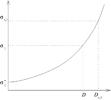
Figure 20: (a) The residual substrate concentration at $E_{101}$ satisfies the relation, $0<\sigma_{1}<\sigma_{f,1}$, precisely when $\sigma_{f,1}>\sigma_{1}^{*}$ and $0<D<D_{c,1}$. (b) Graphical depiction of the conditions for existence of $E_{111}$.

To determine the stability of $E_{101}$, observe that the Jacobian is similar to the matrix

$$\left[\begin{array}[]{ccccc}-c\frac{\partial r_{s,1}}{\partial s_{1}}&-c\frac{\partial r_{s,1}}{\partial e_{1}}&-r_{s,1}&0&Y_{2}r_{s,1}\\ \frac{\partial R_{1}}{\partial s_{1}}&\frac{\partial R_{1}}{\partial e_{1}}&0&\frac{\partial R_{1}}{\partial e_{2}}&\frac{\partial R_{1}}{\partial s_{2}}\\ 0&0&-D&0&0\\ 0&0&0&\frac{\partial R_{2}}{\partial e_{2}}&0\\ 0&0&0&-c\frac{\partial r_{s,2}}{\partial e_{2}}&-D\end{array}\right],$$

which represents the Jacobian of the new system of equations obtained if we make the linear coordinate change

$$\left\{s_{1},s_{2},e_{1},e_{2},c\right\}\longrightarrow\left\{s_{1},e_{1},Y_{1}s_{1}+Y_{1}s_{2}+c,e_{2},s_{2}\right\}.$$

It follows that $E_{101}$ is stable if and only if $\partial R_{2}/\partial e_{2}<0$ and the submatrix

$$\left[\begin{array}[]{cc}-c\frac{\partial r_{s,1}}{\partial s_{1}}&-c\frac{\partial r_{s,1}}{\partial e_{1}}\\ \frac{\partial R_{1}}{\partial s_{1}}&\frac{\partial R_{1}}{\partial e_{1}}\end{array}\right]$$

has negative eigenvalues. One can check that thi submatrix always has negative eigenvalues, and

$$\frac{\partial R_{2}}{\partial e_{2}}=\frac{V_{e,2}\sigma_{f,2}}{\bar{K}_{e,2}}-D-k_{e,2}=D_{t,2}-D,$$

so that $E_{101}$ is stable if and only if

$$D>D_{t,2}.$$ (98)

In the particular case of single-substrate growth on $S_{1}$, this condition is always satisfied, so that $E_{101}$ is stable whenever it exists.

B.2.2 $E_{011}$ ($e_{1}=0$, $e_{2}>0$, $c>0$)

The existence and stability conditions for $E_{011}$ can be derived by methods analogous to those shown above for $E_{101}$.

B.2.3 $E_{111}$ ($e_{1}>0$, $e_{2}>0$, $c>0$)

This steady state exists if and only if the equations

$$0= D(s_{f,1}-s_{1})-V_{s,1}e_{1}\sigma_{1}c$$ (99)

$$0= D(s_{f,2}-s_{2})-V_{s,2}e_{2}\sigma_{2}c$$ (100)

$$0= V_{e,1}\frac{\sigma_{1}}{\bar{K}_{e,1}+e_{1}\sigma_{1}}-\left(Y_{1}V_{s,1}e_{1}\sigma_{1}+Y_{2}V_{s,2}e_{2}\sigma_{2}+k_{e,1}\right)$$ (101)

$$0= V_{e,2}\frac{\sigma_{2}}{\bar{K}_{e,2}+e_{2}\sigma_{2}}-\left(Y_{1}V_{s,1}e_{1}\sigma_{1}+Y_{2}V_{s,2}e_{2}\sigma_{2}+k_{e,2}\right)$$ (102)

$$0= Y_{1}V_{s,1}e_{1}\sigma_{1}+Y_{2}V_{s,2}e_{2}\sigma_{2}-D$$ (103)

have positive solutions, $s_{i},e_{i},c>0$. It follows from (99)–(100) that $c>0$ if and only if $s_{i}<s_{f,i}$.

To prove the existence conditions, it is useful to simplify the above equations. To this end, observe that $c$ can be eliminated from eqs. (99)–(100) to obtain the relation

$$V_{s,2}e_{2}\sigma_{2}\left(s_{f,1}-s_{1}\right) =V_{s,1}e_{1}\sigma_{1}\left(s_{f,2}-s_{2}\right),$$ (104)

and eqs. (101)–(103) immediately yield

$$e_{i}=\frac{V_{e,i}}{D+k_{e,i}}-\frac{\bar{K}_{e,i}}{\sigma_{i}},\;i=i,2,$$ (105)

We conclude that $E_{111}$ exists if and only there exist $0<s_{i}<s_{f,i}$, $e_{i}>0$ satisfying (103)–(105). We show below that such $s_{i}$ and $e_{i}$ exist if and only if $0<D<D_{t,1},D_{t,2},D_{c}$.

To prove the sufficiency of the condition, $0<D<D_{t,1},D_{t,2},D_{c}$, substitute (105) in (103) and (104) to obtain the equations

$$0 =f_{1}(\sigma_{1},\sigma_{2})\equiv\frac{\sigma_{1}}{\overline{\sigma}_{1}}+\frac{\sigma_{2}}{\overline{\sigma}_{2}}=1,$$ (106)

$$0 =f_{2}(\sigma_{1},\sigma_{2})\equiv\frac{V_{s,1}V_{e,1}}{D+k_{e,1}}\left(\sigma_{1}-\underline{\sigma}_{1}\right)\left(s_{f,2}-s_{2}\right)-\frac{V_{s,2}V_{e,2}}{D+k_{e,2}}\left(\sigma_{2}-\underline{\sigma}_{2}\right)\left(s_{f,1}-s_{1}\right),$$ (107)

where

$$\overline{\sigma}_{i} \equiv\frac{1}{Y_{i}V_{s,i}\bar{K}_{e,i}}\left(D+k_{e,i}\right)\left(D+Y_{1}V_{s,1}\bar{K}_{e,1}+Y_{2}V_{s,2}\bar{K}_{e,2}\right),$$

$$\underline{\sigma}_{i} \equiv\left(D+k_{e,i}\right)\frac{\bar{K}_{e,i}}{V_{e,i}}.$$

Now, (106) defines a line on the $\sigma_{1},\sigma_{2}$-plane with the intercepts, $\overline{\sigma}_{1}$ and $\overline{\sigma}_{2}$ (full line in Fig. 20b). As $D$ increases, it moves further from the origin, and passes through the point, $\left(\sigma_{f,1},\sigma_{f,2}\right)$, precisely when $D=D_{c}$. On the other hand, (107) defines a curve which has the geometry of the dashed curve in Fig. 20b. To see this, observe that $\left(\underline{\sigma}_{1},\underline{\sigma}_{2}\right)$ and $\left(\sigma_{f,1},\sigma_{f,2}\right)$ lie on the curve. Moreover, $\left(\underline{\sigma}_{1},\underline{\sigma}_{2}\right)$ lies to the left and below $\left(\sigma_{f,1},\sigma_{f,2}\right)$ because

$$D<D_{t,i}=\frac{V_{e,i}\sigma_{f,i}}{\bar{K}_{e,i}}-k_{e,i}\Leftrightarrow\underline{\sigma}_{i}<\sigma_{f,i},$$

and the slope of the curve is positive since

$$-\frac{\partial f_{1}/\partial\sigma_{1}}{\partial f_{1}/\partial\sigma_{2}}=\frac{\frac{V_{s,1}V_{e,2}}{D+k_{e,2}}\frac{ds_{1}}{d\sigma_{1}}\left(\sigma_{2}-\underline{\sigma}_{2}\right)+\frac{V_{s,2}V_{e,1}}{D+k_{e,1}}\left(s_{f,2}-s_{2}\right)}{\frac{V_{s,2}V_{e,1}}{D+k_{e,1}}\frac{ds_{2}}{d\sigma_{2}}\left(\sigma_{1}-\underline{\sigma}_{1}\right)+\frac{V_{s,1}V_{e,2}}{D+k_{e,2}}\left(s_{f,1}-s_{1}\right)}>0$$

for all $\underline{\sigma}_{i}<\sigma_{i}<\sigma_{f,i}$. Finally, $\left(\underline{\sigma}_{1},\underline{\sigma}_{2}\right)$ lies below the growth isocline because

$$\frac{\underline{\sigma}_{1}}{\overline{\sigma}_{1}}+\frac{\underline{\sigma}_{2}}{\overline{\sigma}_{2}}=\frac{Y_{1}V_{s,1}\bar{K}_{e,1}+Y_{2}V_{s,2}\bar{K}_{e,2}}{D+Y_{1}V_{s,1}\bar{K}_{e,1}+Y_{2}V_{s,2}\bar{K}_{e,2}}<1$$

for all $D>0$. It follows that the curves defined by (106) and (107) intersect at a unique point, say, $\left(\widetilde{\sigma}_{1},\widetilde{\sigma}_{2}\right)$, such that $\underline{\sigma}_{i}<\widetilde{\sigma}_{1}<\sigma_{f,1}.$ Since

$$\underline{\sigma}_{i}<\widetilde{\sigma}_{i}\Leftrightarrow e_{i}=\frac{V_{e,i}}{D+k_{e,i}}-\frac{\bar{K}_{e,i}}{\widetilde{\sigma}_{i}}>0$$

$E_{111}$ exists and is unique.

The necessity of the existence conditions follows from the fact that for all $0<\sigma_{i}<\sigma_{f,i}$,

$$e_{i}<\frac{V_{e,i}}{D+k_{e,i}}-\frac{\bar{K}_{e,i}}{\sigma_{f,i}}=\frac{\bar{K}_{e,i}}{\sigma_{i}\left(D+k_{e,i}\right)}\left(D_{t,i}-D\right).$$

Hence, if $D_{t,i}\leq 0$ or $D\geq D_{t,i}$, $E_{111}$ does not exist because $e_{i}<0$. Likewise, if $D\geq D_{c}$, $E_{111}$ does not exist because there are no $0<s_{i}<s_{f,i}$ satisfying (106).

We conclude that $E_{111}$ exists if and only if

$$0<D<D_{t,1},D_{t,2},D_{c}.$$

We were unable to prove the stability condition for $E_{111}$. However, extensive numerical simulations suggest that it is stable whenever it exists.

References

- Adhya (2003) Adhya, S., Jun 2003. Suboperonic regulatory signals. Sci STKE 2003 (185), pe22.
- Bally et al. (1994) Bally, M., Wilberg, E., Kühni, M., Egli, T., 1994. Growth and regulation of enzyme synthesis in the nitrilotriacetic acid (NTA)-degrading bacterium Chelatobacter heintzii ATCC 29600. Microbiology 140, 1927–1936.
- Brinkmann and Babel (1992) Brinkmann, U., Babel, W., 1992. Simultaneous utilization of heterotrophic substrates by Hansenula polymorpha results in enhanced growth. Adv. Microbiol. Biotechnol. 37, 98–103.
- Buettner et al. (1973) Buettner, M. J., Spitz, E., Rickenberg, H. V., Jun 1973. Cyclic adenosine 3’,5’-monophosphate in Escherichia coli. J Bacteriol 114 (3), 1068–1073.
- Carroll et al. (2005) Carroll, S. B., Grenier, J. K., Weatherbee, S. D., 2005. From DNA to Diversity: Molecular Genetics and the Evolution of Animal Design, 2nd Edition. Blackwell Publishing.
- Chauvaux (1996) Chauvaux, S., 1996. CcpA and HPr(ser-P): mediators of catabolite repression in Bacillus subtilis. Res Microbiol 147 (6-7), 518–522.
- Clarke et al. (1968) Clarke, P. H., Houldsworth, M. A., Lilly, M. D., 1968. Catabolite repression and the induction of amidase synthesis by Pseudomonas aeruginosa 8602 in continuous culture. J. Gen. Microbiol. 51, 225.
- Collier et al. (1996) Collier, D. N., Hager, P. W., Phibbs, P. V., 1996. Catabolite repression control in the pseudomonads. Res Microbiol 147 (6-7), 551–561.
- Danchin et al. (1981) Danchin, A., Dondon, L., Joseph, E., Ullmann, A., 1981. Transcription-translation coupling and polarity: A possible role of cyclic amp. Biochimie 63 (5), 419–424.
- Dean (1972) Dean, A. C. R., 1972. Influence of environment on the control of enzyme synthesis. J. Appl. Chem. Biotechnol. 22, 245–259.
- Dedem and Moo-Young (1975) Dedem, G. V., Moo-Young, M., 1975. A model for diauxic growth. Biotechnol. Bioeng. 17, 1301–1312.
- Eggeling and Sahm (1981) Eggeling, L., Sahm, H., 1981. Enhanced utilization of methanol during growth on mixed substrates: A continuous culture study with Hansenula polymorpha. Arch. Microbiol. 14, 305–386.
- Egli (1995) Egli, T., 1995. The ecological and physiological significance of the growth of heterotrophic microorganisms with mixtures of substrates. Adv. Microbiol. Ecol. 14, 305–386.
- Egli et al. (1986) Egli, T., Bosshard, C., Hamer, G., 1986. Simultaneous utilization of methanol-glucose mixtures by Hansenula polymorpha in chemostat: Influence of dilution rate and mixture composition on utilization pattern. Biotechnol. Bioeng. 28, 1735–1741.
- Egli and Harder (1983) Egli, T., Harder, W., 1983. Growth of methylotrophs on mixed substrates. In: Crawford, R. L. (Ed.), Microbial growth on C1 compounds. ASM Press, pp. 330–337.
- Egli et al. (1982a) Egli, T., Käppeli, O., Fiechter, A., 1982a. Mixed substrate growth of methylotrophic yeasts in chemostat culture: Influence of dilution rate on the utilization of a mixture of methanol and glucose. Arch. Microbiol. 131, 8–13.
- Egli et al. (1982b) Egli, T., Käppeli, O., Fiechter, A., 1982b. Regulatory flexibility of methylotrophic yeasts in chemostat culture: Simultaneous assimilation of glucose and methanol at a fixed dilution rate. Arch. Microbiol. 131, 1–7.
- Egli et al. (1993) Egli, T., Lendenmann, U., Snozzi, M., 1993. Kinetics of microbial growth with mixtures of carbon sources. Antonie van Leeuwenhoek 63, 289–298.
- Egli et al. (1980) Egli, T., van Dijken, J. P., Veenhuis, J. P., Harder, W., Fiechter, A., 1980. Methanol metabolism in yeasts: Regulation of the synthesis of catabolic enzymes. Arch. Microbiol. 124, 115–121.
- Epstein et al. (1975) Epstein, W., Rothman-Denes, L. B., Hesse, J., Jun 1975. Adenosine 3’:5’-cyclic monophosphate as mediator of catabolite repression in Escherichia coli. Proc Natl Acad Sci U S A 72 (6), 2300–2304.
- Eraso and Gancedo (1984) Eraso, P., Gancedo, J. M., May 1984. Catabolite repression in yeasts is not associated with low levels of cAMP. Eur J Biochem 141 (1), 195–198.
- Ferenci (1996) Ferenci, T., Jul 1996. Adaptation to life at micromolar nutrient levels: the regulation of Escherichia coli glucose transport by endoinduction and cAMP. FEMS Microbiol Rev 18 (4), 301–317.
- Fredrickson (1976) Fredrickson, A. G., 1976. Formulation of structured growth models. Biotechnol. Bioeng. 28, 1481–1486.
- Guidi-Rontani et al. (1984) Guidi-Rontani, C., Danchin, A., Ullmann, A., 1984. Transcriptional control of polarity in Escherichia coli by cAMP. Mol Gen Genet 195 (1-2), 96–100.
- Harder and Dijkhuizen (1976) Harder, W., Dijkhuizen, L., 1976. Mixed substrate utilization. In: Dean, A. C. R., Ellwood, D. C., Evans, C. G. T., Melling, J. (Eds.), Continuous Culture 6: Applications and New Fields. Ellis Horwood, Chichester, Ch. 23, pp. 297–314.
- Harder and Dijkhuizen (1982) Harder, W., Dijkhuizen, L., 1982. Strategies of mixed substrate utilization in microorganisms. Philos. Trans. R. Soc. London B 297, 459–480.
- Hartner and Glieder (2006) Hartner, F. S., Glieder, A., 2006. Regulation of methanol utilisation pathway genes in yeasts. Microb Cell Fact 5, 39.
- Herbert et al. (1956) Herbert, D., Elsworth, R., Telling, R. C., 1956. The continuous culture of bacteria: A theoretical and experimental study. J. Gen. Microbiol. 14, 601–622.
- Hogema et al. (1998) Hogema, B. M., Arents, J. C., Bader, R., Eijkemans, K., Inada, T., Aiba, H., Postma, P. W., May 1998. Inducer exclusion by glucose 6-phosphate in Escherichia coli. Mol Microbiol 28 (4), 755–765.
- Inada et al. (1996) Inada, T., Kimata, K., Aiba, H., 1996. Mechanism responsible for the glucose-lactose diauxie in Escherichia coli: Challenge to the cAMP model. Genes Cells 1, 293–301.
- Jacob and Monod (1961) Jacob, F., Monod, J., 1961. Genetic regulatory mechanisms in the synthesis of proteins. J. Mol. Biol. 3, 318–356.
- Johnston (1999) Johnston, M., Jan 1999. Feasting, fasting and fermenting. glucose sensing in yeast and other cells. Trends Genet 15 (1), 29–33.
- Kimata et al. (1997) Kimata, K., Takahashi, H., Inada, T., Postma, P., Aiba, H., 1997. cAMP receptor protein-cAMP plays a crucial role in glucose-lactose diauxie by activating the major glucose transporter gene in Escherichi coli. Proc. Nat. Acad. Sci. USA 94, 12914–12919.
- Kovar et al. (2002) Kovar, K., Chaloupka, V., Egli, T., 2002. A threshold concentration is required to initiate the degradation of 3-phenylpropionic acid in Escherichia coli. Acta Biotechnologica 22 (3–4), 285–298.
- Kovarova et al. (1997) Kovarova, K., Kach, A., Egli, T., Zehnder, A., 1997. Cultivation of Escherichia coli with mixtures of 3-phenylpropionic aicd and glucose: Steady state growth kinetics. Appl. Environ. Microbiol. 63, 2619–2624.
- Kovarova-Kovar and Egli (1998) Kovarova-Kovar, K., Egli, T., 1998. Growth kinetics of suspended microbial cells: From single-substrate-controlled growth to mixed-substrate kinetics. Microbiol. Mol. Biol. Rev. 62, 646–666.
- Kovárová et al. (1996) Kovárová, K., Zehnder, A. J., Egli, T., Aug 1996. Temperature-dependent growth kinetics of Escherichia coli ML 30 in glucose-limited continuous culture. J Bacteriol 178 (15), 4530–4539.
- Kremling et al. (2001) Kremling, A., Bettenbrock, K., Laube, B., Jahreis, K., Lengeler, J. W., Gilles, E. D., Oct 2001. The organization of metabolic reaction networks. III. Application for diauxic growth on glucose and lactose. Metab Eng 3 (4), 362–379.
- Kuo et al. (2003) Kuo, J.-T., Chang, Y.-J., Tseng, C.-P., Oct 2003. Growth rate regulation of lac operon expression in Escherichia coli is cyclic AMP dependent. FEBS Lett 553 (3), 397–402.
- Lendenmann (1994) Lendenmann, U., 1994. Growth kinetics of Escherichia coli with mixtures of sugars. Ph.D. thesis, Swiss Federal Institute of Technology, Zürich, Switzerland.
- Lendenmann et al. (1996) Lendenmann, U., Snozzi, M., Egli, T., 1996. Kinetics of the simultaneous utilization of sugar mixtures by Escherichia coli in continuous culture. Appl. Environ. Microbiol. 62, 1493–1499.
- Mach et al. (1984) Mach, H., Hecker, M., Mach, F., 1984. Evidence for the presence of cyclic adenosine monophosphate in Bacillus subtilis. FEMS Microbiol 22, 27–30.
- Mandelstam (1958) Mandelstam, J., May 1958. Turnover of protein in growing and non-growing populations of escherichia coli. Biochem J 69 (1), 110–119.
- Matin (1978) Matin, A., 1978. Microbial regulatory mechanisms at low nutrient concentrations as studied in a chemostat. In: Shilo, M. (Ed.), Strategies of Microbial Life in Extreme Environments. Verlag Chemie, Weinheim, pp. 323–339.
- McGinnis and Paigen (1969) McGinnis, J. F., Paigen, K., Nov 1969. Catabolite inhibition: a general phenomenon in the control of carbohydrate utilization. J Bacteriol 100 (2), 902–913.
- Monod (1942) Monod, J., 1942. Recherches sur la croissance des cultures bactériennes [Studies on the growth of bacterial cultures]. Actualités Scientifique et Industrielles 911, 1–215.
- Monod (1947) Monod, J., 1947. The phenomenon of enzymatic adaptation and its bearings on problems of genetics and cellular differentiation. Growth 11, 223–289.
- Morales et al. (2004) Morales, G., Linares, J. F., Beloso, A., Albar, J. P., Martínez, J. L., Rojo, F., Mar 2004. The Pseudomonas putida Crc global regulator controls the expression of genes from several chromosomal catabolic pathways for aromatic compounds. J Bacteriol 186 (5), 1337–1344.
- Müller-Hill (1996) Müller-Hill, B., 1996. The lac operon, 1st Edition. de Gruyter, Berlin.
- Murray (1989) Murray, J. D., 1989. Mathematical Biology. Biomathematics Texts. Springer-Verlag, New York.
- Narang (1998a) Narang, A., 1998a. The dynamical analogy between microbial growth on mixtures of substrates and population growth of competing species. Biotech Bioeng 59, 116–121.
- Narang (1998b) Narang, A., 1998b. The steady states of microbial growth on mixtures of substitutable substrates in a chemostat. J Theor Biol 190, 241–261.
- Narang (2006) Narang, A., Sep 2006. Comparative analysis of some models of gene regulation in mixed-substrate microbial growth. J Theor Biol 242 (2), 489–501.
- Narang et al. (1997) Narang, A., Konopka, A., Ramkrishna, D., 1997. New patterns of mixed substrate growth in batch cultures of Escherichia coli K12. Biotech Bioeng 55, 747–757.
- Narang and Pilyugin (2007a) Narang, A., Pilyugin, S. S., 2007a. Bacterial gene regulation in diauxic and nondiauxic growth. J. Theoret. Biol. 244, 326–348.
- Narang and Pilyugin (2007b) Narang, A., Pilyugin, S. S., October 2007b. Bistability of the lac operon during growth of Escherichia coli on lactose or lactose + glucose., Bull. Math. Biol., accepted.
- Ng and Dawes (1973) Ng, F. M., Dawes, E. A., Feb 1973. Chemostat studies on the regulation of glucose metabolism in Pseudomonas aeruginosa by citrate. Biochem J 132 (2), 129–140.
- Notley-McRobb and Ferenci (2000) Notley-McRobb, L., Ferenci, T., Aug 2000. Substrate specificity and signal transduction pathways in the glucose-specific enzyme II (EII(Glc)) component of the Escherichia coli phosphotransferase system. J Bacteriol 182 (16), 4437–4442.
- Perlman and Pastan (1968) Perlman, R. L., Pastan, I., Oct 1968. Regulation of -galactosidase synthesis in Escherichia coli by cyclic adenosine 3’,5’-monophosphate. J Biol Chem 243 (20), 5420–5427.
- Postma et al. (1993) Postma, P. W., Lengeler, J. W., Jacobson, G. R., Sep 1993. Phosphoenolpyruvate:carbohydrate phosphotransferase systems of bacteria. Microbiol Rev 57 (3), 543–594.
- Ptashne and Gann (2002) Ptashne, M., Gann, A., 2002. Genes & Signals. Cold Spring Harbor Laboratory Press, Cold Spring Harbor, New York.
- Rudolph and Grady (2001) Rudolph, J. M., Grady, C. P., Sep 2001. Effect of media composition on yield values of bacteria growing on binary and ternary substrate mixtures in continuous culture. Biotechnol Bioeng 74 (5), 396–405.
-
Rudolph and Grady (2002)
Rudolph, J. M., Grady, C. P. L., Jul 2002. Catabolic enzyme levels
in bacteria
grown on binary and ternary substrate mixtures in continuous culture.
Biotechnol Bioeng 79 (2), 188–199.
URL http://dx.doi.org/10.1002/bit.10276 - Santillán et al. (2007) Santillán, M., Mackey, M. C., Zeron, E. S., Jun 2007. Origin of bistability in the lac operon. Biophys J 92 (11), 3830–3842.
- Savageau (2001) Savageau, M. A., Mar 2001. Design principles for elementary gene circuits: Elements, methods, and examples. Chaos 11 (1), 142–159.
- Schmidt and Alexander (1985) Schmidt, S. K., Alexander, M., Apr 1985. Effects of dissolved organic carbon and second substrates on the biodegradation of organic compounds at low concentrations. Appl Environ Microbiol 49 (4), 822–827.
- Schmidt et al. (1987) Schmidt, S. K., Scow, K. M., Alexander, M., Nov 1987. Kinetics of p-nitrophenol mineralization by a Pseudomonas sp.: Effects of second substrates. Appl Environ Microbiol 53 (11), 2617–2623.
- Seeto et al. (2004) Seeto, S., Notley-McRobb, L., Ferenci, T., Apr 2004. The multifactorial influences of RpoS, Mlc and cAMP on ptsG expression under glucose-limited and anaerobic conditions. Res Microbiol 155 (3), 211–215.
- Silver and Mateles (1969) Silver, R. S., Mateles, R. I., 1969. Control of mixed-substrate utilization in continuous cultures of Escherichia coli. J. Bacteriol. 97, 535–543.
- Smith and Atkinson (1980) Smith, S. S., Atkinson, D. E., Jul 1980. The expression of -galactosidase by Escherichia coli during continuous culture. Arch Biochem Biophys 202 (2), 573–581.
- Toda (1981) Toda, K., 1981. Induction and repression of enzymes in microbial cultures. J. Chem. Tech. Biotechnol. 31, 775–790.
- Ullmann (1974) Ullmann, A., Mar 1974. Are cyclic AMP effects related to real physiological phenomena? Biochem Biophys Res Commun 57 (2), 348–352.
- Ullmann and Monod (1968) Ullmann, A., Monod, J., Nov 1968. Cyclic AMP as an antagonist of catabolite repression in Escherichia coli. FEBS Lett 2 (1), 57–60.
- Wanner et al. (1978) Wanner, B. L., Kodaira, R., Neidhardt, F. C., Dec 1978. Regulation of lac operon expression: Reappraisal of the theory of catabolite repression. J Bacteriol 136 (3), 947–954.
- Weickert and Adhya (1993) Weickert, M. J., Adhya, S., Oct 1993. The galactose regulon of Escherichia coli. Mol Microbiol 10 (2), 245–251.
- Winkler and Wilson (1967) Winkler, H. H., Wilson, T. H., 1967. Inhibition of -galactoside transport by substrates of the glucose transport system in Escherichia coli. Biochim Biophys Acta 135 (5), 1030–1051.
- Wong et al. (1997) Wong, P., Gladney, S., Keasling, J. D., 1997. Mathematical model of the lac operon: inducer exclusion, catabolite repression, and diauxic growth on glucose and lactose. Biotechnol Prog 13 (2), 132–143.
- Yagil and Yagil (1971) Yagil, G., Yagil, E., 1971. On the relation between effector concentration and the rate of induced enzyme synthesis. Biophys. J. 11, 11–27.