Hot QCD equations of state and response functions for quark-gluon plasma

Abstract

We study the response functions (chromo-electric susceptibilities) of quark-gluon plasma as a function of temperature in the presence of interactions. We consider two equations of state for hot QCD. The first one is fully perturbative, of $O(g^{5})$ EOS and, and the second one which is $O[g^{6}\ln(1/g)+\delta]$, incorporates some non-perturbative effects. Following a recent work (Physical Review C 76, 054909(2007)), the interaction effects contained in the EOS are encapsulated in terms of effective chemical potentials($\tilde{\mu}$) in the equilibrium distribution functions for the partons.By using them in another recent formulation of the response functions(arXiv:0707.3697), we determine explicitly the chromo-electric susceptibilities for QCD plasma. We find that it shows large deviations from the ideal behavior. We further study the modification in the heavy quark potential due to the medium effects. In particular, we determine the temperature dependence of the screening lengths by fixing the effective coupling constant $Q$ which appears in the transport equation by comparing the screening in the present formalism with exact lattice QCD results. Finally, we study the dissociation phenomena of heavy quarkonium states such as $c\bar{c}$ and $b\bar{b}$, and determine the dissociation temperatures. Our results are in good agreement with recent lattice results.

Keywords:   Response function; non-Abelian permittivity; Quark-Gluon plasma; hot QCD equation of state; equilibrium distribution function; chemical potential; RHIC.

PACS: 25.75.-q; 24.85.+p; 05.20.Dd; 12.38.Mh

I Introduction

It is expected that at high temperatures ($T\sim 150-200MeV$) and high densities ($\rho\sim 10Gev/fm^{3}$) nuclear matter undergoes a deconfinement transition to the quark-gluonic phase. This phase is under intense investigation in heavy ion collisions, and already, interesting results have been reported by Relativistic Heavy Ion Collider(RHIC) experiments expt . As an important development, flow measurementsstar-report suggest that close to the transition temperature $T_{c}$, the quark-gluon plasma (QGP) phase is strongly interacting — showing an almost perfect liquid behavior, with very low viscosity to entropy ratio — rather than showing a behavior close to that of an ideal gas. See Ref. new-matter for a comprehensive review of experimental observations from RHIC, and Ref. expt ; exp-status1 ; exp-status2 ; s-a-bass ; csorgo for other recent experimental results. On the other hand, lattice computations lattice ; lattice-new also suggest that QGP is strongly interacting even at $T=2T_{c}$. This finding has been reproduced by a number of other theoretical studies — by employing AdS/CFT correspondence in the strongly interacting regime of QCDdtson , by molecular dynamical simulations for classical strongly coupled systemsshuryak , and by model calculations with Au-Au data from RHIC bair ; jyo .

If this be the case, as it indeed appears to be, then the plasma interactions would be largely in the non-perturbative regime; in this regime, few analytic techniques are available for a robust theoretical analysis. Effective interaction approaches are needed. In this direction, considerable work has already been done and we refer the reader to Ref. matsui ; elze ; vr1 ; vr2 ; akranjan ; shur2 ; shur3 ; blaizot1 for some of the theoretical results.

The effective approaches emphasize the collective origin of the plasma properties which can be best understood within a semi-classical framework. Indeed, in a recent work fluid , the successes of hydrodynamics in interpreting and understanding the experimental observations from RHIC has been reviewed. Since more exciting and discerning data is expected from LHC experiments soon, and given the above context, it is worthwhile exploring semi-classical techniques to understand the properties of QGP in heavy ion collisions. In this context, it is known by now pisarski ; braaten-1 ; braaten-2 ; nair that a classical behavior emerges naturally when one considers hard thermal loop(HTL) contributions. A local formulation of HTL effective action has been obtained by Blaizot and Iancu who have succeeded in rewriting the HTL effective theory as a kinetic theory with a Vlasov term blaizot ; blaizot-2 ; blaizot-3 ; blaizot-4 . A significant development in this direction is the realization that the HTL effects are, in fact, essentially classical and that they are much easier to handle within the frame work of classical transport equations cm1 ; cm4 ; cristina . Thus, the semi-classical techniques appear hold the promise of providing tools to understand the bulk properties of QGP.

The present paper continues the theme, and its central aim is to combine the kinetic equation approach which yields the transport properties, with the hot QCD equations of state to make predictions which can be perhaps tested in heavy ion collisions. Recently, Ranjan and Ravishankar have developed a systematic approach to determine fully the response functions of QGP, with a special emphasis on the color charge as a dynamical variable akranjan . In parallel, Chandra, Kumar and Ravishankar have succeeded in adapting two hot QCD EOS to make predictions for heavy ion collisions chandra1 . They have shown that the interaction effects which modify the equations of state can be expressed by absorbing them into effective fugacities ($z_{q,g}$) of otherwise free or weakly interacting quasi quarks and gluons. Since the analysis in Ref. (akranjan ) was illustrated only for (the academically interesting) case of ideal quarks and gluons, it is but natural to bring the two studies together and explore what the hot QCD EOS have to predict for heavy ion collisions. We take up this program in this paper.

The main result of this paper is the determination of the modification that the heavy quark potential undergoes in a medium constituted by interacting QGP, as predicted by the two EOS which we consider. After determining the screening length as a function of temperature, we focus on the Cornell potentialcornell and study the dissociation mechanism for $c\bar{c}$ and $b\bar{b}$ states. The results are rather surprising and may as well signal the inapplicability of these EOS to describe the deconfined phase. On the other hand, if the transition from the confined to the deconfined state is not a phase transition as several studies predict phaseT , it may still be possible to attribute some physical significance to the predictions of these EOS. We undertake the project here. We show that, by using one of the phenomenological EOS is quite a good approximation to the more rigorous lattice results, the value of the phenomenological coupling constant that occurs in the Boltzmann equation can be fixed. Ultimately, the physical viability or otherwise of the results need to be established by comparing them repeating the analysis of chandra1 with the lattice EOS. That will be taken up in a separate paper.

We consider two specific hot QCD equations of state: The first, which we call EOS1 is perturbative, with contributions up to $O(g^{5})$arnold ; zhai . The second EOS has a free parameter $\delta$, and is evaluated upto $O[g^{6}\log(1/g)]$kaj1 . We denote it by EOS$\delta$. $\delta$ may be fine tuned to get a reasonably good agreement kaj1 with the lattice results fkarsch , which we exploit here. Both the EOS are expected to be valid for $T>2T_{c}$ kaj1 , and EOS$\delta$ is reliable beyond $T\sim 4T_{c}$.

The paper is organized as follows: In section II, we introduce the two hot QCD equations of state and outline the recently developed methodchandra1 to adapt them for making definite predictions for QGP at RHIC and the forthcoming experiments at LHC. In section III, we obtain the expressions for the response functions of interacting QGP and in section IV, we study their temperature dependence in detail. In section V, we study the modifications in heavy quark potential due to the hot QCD medium. We further study the temperature dependence of the Debye screening lengths in hot QCD. We investigate the “melting phenomena” of heavy quarkonia such as $J/\Psi$ and $b\bar{b}$ in the medium, and extract the dissociation temperature. In doing so we also relate the phenomenological charge that occurs in the transport equation to lattice and experimental observables. We conclude the paper in section VI.

II Hot QCD equations of state and their quasi-particle description

There are various equations of state proposed for QGP at RHIC. These include non-perturbative lattice EOS fkarsch , hard thermal loop(HTL) resumed EOShtleos and perturbative hot QCD equations of state zhai ; arnold ; kaj1 . In the present paper, we seek to determine the chromo-electric response functions for QGP by employing two EOS: (i) the fully perturbative $O(g^{5})$ hot QCD EOS proposed by Arnold and Zhaiarnold and Zhai and Kastening zhai , and (ii) The EOS of $O[g^{6}(\ln(1/g)+\delta)]$ determined by Kajantie et al kaj1 , by incorporating contributions from non-perturbative scales, $gT$ and $g^{2}T$. We employ the method recently formulated by Ranjan and Ravishankarakranjan to extract the chromo-electric permittivities of the medium. EOS1 reads

$$P_{g^{5}} = \frac{8\pi^{2}}{45\beta^{4}}\bigg{\{}(1+\frac{21N_{f}}{32})-\frac{15}{4}(1+\frac{5N_{f}}{12})\frac{\alpha_{s}}{\pi}+30(1+\frac{N_{f}}{6})(\frac{\alpha_{s}}{\pi})^{\frac{3}{2}}$$

$$+\bigg{[}(237.2+15.97N_{f}-0.413N_{f}^{2}+\frac{135}{2}(1+\frac{N_{f}}{6})\ln(\frac{\alpha_{s}}{\pi}$$

$$\times(1+\frac{N_{f}}{6}))\frac{165}{8}(1+\frac{5N_{f}}{12})(1-\frac{2N_{f}}{33})\ln[\frac{\mu_{MS}\beta}{2\pi}]\bigg{]}(\frac{\alpha_{s}}{\pi})^{2}$$

$$+(1+\frac{N_{f}}{6})^{\frac{1}{2}}\bigg{[}-799.2-21.99N_{f}-1.926N_{f}^{2}$$

$$+\frac{495}{2}(1+\frac{N_{f}}{6})(1+\frac{2N_{f}}{33})\ln[\frac{\mu_{MS}\beta}{2\pi}]\bigg{]}(\frac{\alpha_{s}}{\pi})^{\frac{5}{2}}\bigg{\}}$$

$$+O(\alpha_{s})^{3}\ln(\alpha_{s})).$$

while EOS$\delta$ is given by

$$P_{g^{6}\ln(1/g)} = P_{g^{5}}+\frac{8\pi^{2}}{45}T^{4}\biggl{[}1134.8+65.89N_{f}+7.653N_{f}^{2}$$ (2)

$$-\frac{1485}{2}\left(1+\frac{1}{6}N_{f}\right)\left(1-\frac{2}{33}N_{f}\right)\ln(\frac{\mu_{MS}}{2\pi T})\biggr{]}$$

$$\times\left(\frac{\alpha_{s}}{\pi}\right)^{3}(\ln\frac{1}{\alpha_{s}}+\delta).$$

As mentioned earlier, $\delta$ is an empirical parameter, introduced to incorporate phenomenologically the undetermined contributions at $O(g^{6})$. It also acts as a fitting parameter to get the best agreement with the lattice results.

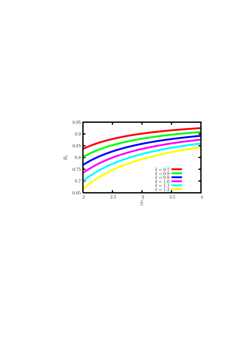
Figure 1: (Color online) Relative equation of state(wrt ideal EOS) for pure gauge theory plasma as a function of $T/T_{c}$ for various values of $\delta$.

.

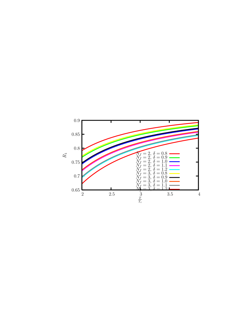
Figure 2: (Color online) Relative equation of statewrt ideal EOS for full QCD plasma with $N_{f}=2,3$ as a function of $T/T_{c}$ for various values of $\delta$.

.

II.1 The underlying distribution functions

The construction of the distribution functions that underlie the EOS, in terms of effective quarks and gluons which act as quasi-excitations, has been discussed by Chandra et. al., chandra1 in the specific context of EOS1 and EOS$\delta$. To review the method briefly, all the terms that represent interactions are collected together by recasting them as effective fugacities ($z_{q,g}\equiv\exp(\mu_{q,g})$) for the otherwise free quarks and gluons. Of course, the pure gague theory case is simply obtained by putting the number of flavors, $N_{F}=0$ in the EOS. Thus, $\mu_{g}$ represents the self interactions of the gluons, while $\mu_{f}$ encapsulates the quark-quark and the quark gluon interaction terms. Importantly, the two EOS of interest to us are valid when $T>2T_{c}$, and in this range, the quantities $\tilde{\mu}_{q,g}\equiv\beta\mu_{q,g}$ are perturbative parameters. Thus, it is possible to solve for $\tilde{\mu}_{f,g}$ self consistently through a systematic iterative procedure. In this procedure, all the temperature effects are contained in the effective fugacities $z\equiv z(\alpha_{s}(T/T_{c}))$, where we display the dependence on the temperature and coupling constant explicitly. It has been shown in Ref. chandra1 (where the details can be found) that one can trade off the dependence of the effective fugacities on the renormalization scale ( $\mu_{\bar{MS}}$) by their dependence on the critical temperature $T_{c}$. For that purpose, one utilizes the one loop expression of $\alpha_{s}(T)$ at finite temperature given by shaung

$$\alpha_{s}(T) = \frac{1}{8\pi b_{0}\log(T/\lambda_{T})}=\alpha_{s}(\mu^{2})|_{\mu=\mu_{\bar{MS}}(T)}$$

$$\mu_{\bar{M}S}(T) = 4\pi T\exp(-(\gamma_{E}+1/22))$$

$$\lambda_{T} = \frac{\exp(\gamma_{E}+1/22)}{4\pi}\lambda_{MS}.$$

employing which the dependence on $\mu_{\bar{MS}}$ is eliminated, in favor of $T_{c}$. Consequently, the effective chemical potentials get to depend only on $T/T_{c}$. Note that effective fugacities have merely been introduced to capture the interaction effects present in hot QCD equations of state.

Once the distribution functions are in hand, the study of transport properties is a straight forward exercise if we employ the analysis put forth by Ranjan et. al. akranjan .

In Figs. 1 and 2, we display the behavior of EOS$\delta$ for various values of the parameter $\delta$. The figures show the pure gauge theory contributions to the EOS and full QCD separately. We remark parenthetically that the studies in the earlier work chandra1 were confined to EOS1 and the special case $\delta=0$ in EOS$\delta$. For the details on EOS1 and EOS$\delta$ for $\delta=0$, we refer the reader to Ref. chandra1 (see Fig.1-7 of Ref.chandra1 ). First of all, we see that as $\delta$ increases in magnitude, the EOS, for both pure gauge theory and full QCD, become softer, with $P/P_{I}$ taking smaller values, we denote the the ratio $P/P_{I}$ by $R_{1}$. Kajantiekaj1 obtains the best fit with the lattice results of Boyd et. al.boyd by choosing a value $\delta=0.7$. We find that to get agreement with the more recent results of Karsch fkarsch , $\delta\approx 1.0$ is preferred, when we consider $T>2T_{c}$. In short, we find that the range of values $0.8\leq\delta\leq 1.2$ gives a reasonably good qualitative agreement with the lattice results for the screening lengths.

Here, we wish to mention that there is an uncertainty in fixing the free parameter $\delta$. This follows from the freedom in choosing the QCD renormalization scale at high temperature. This has been investigated in detail by Blaizot, Iancu and Rebhan rebh . The value of $\delta$ in the present paper has been obtained by employing the one loop expression for the running coupling constant and the QCD renormalization scale determined in Ref.shaung . We intend to study the quasi-particle content of HTL and HDL equations of staterebh ; rebh1 and lattice equation of state in future.

The behavior of the corresponding fugacities, as a function of temperature, is shown in Fig.3. It may be seen that $0<z_{g,q}<1.0$ which ensures the convergence of the method to determine the effective fugacities from the hot QCD EOS. We now proceed to determine the response of the plasma in the next section.

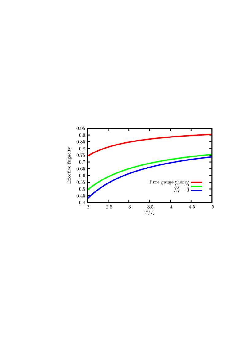
Figure 3: (Color online) Effective parton fugacities $(z_{g,q})$ quarks determined from EOS$\delta$ as a function of temperature. Note that the behavior is shown for $\delta=1.0$.

.

III Response functions for interacting qgp

Recently Ranjan and Ravishankar akranjan have determined the form of chromo-electric response functions for collision less quark-gluon plasma within the framework of semi-classical transport theory. They have set up the transport equation in the extended phase space including the SU(3) group space corresponding to dynamical color degree of freedom. They have taken the distribution function in a coherent state basis defined over the extended single particle phase space $\mathcal{R}^{6}\otimes\mathcal{C}_{\mathcal{G}}$, where $\mathcal{C}_{\mathcal{G}}=\mathcal{G}/\mathcal{H}$ is the phase space corresponding to the color degree of freedom, obtained as a coset space by factoring the group space by the stabilizer group $\mathcal{H}$ of any reference state in the Hilbert space. Having been employed to study the ideal case, the formalism has not been applied to examine the behavior of the plasma with a realistic EOS. We employ the results of the previous section and rectify this drawback, by incorporating the interaction effects as represented by EOS1 and EOS$\delta$.

A brief comment on the response functions. In contrast to electrodynamic plasma, the chromo-electric response has a richer structure. Apart from the standard permittivity which we shall call Abelian and denote by $\epsilon_{A}$, there are additional response functions, their number depending on the color carried by the partons. Thus, quarks have an additional response function which affects the non-Abelian coupling. The corresponding permittivity will be called non-Abelian, and denoted by $\epsilon_{N}$. The two functions exhaust the response in the quark sector. The gluonic sector, arising from the adjoint representation of the gauge group admits yet another kind of response, corresponding to tensor excitations. These excitations are not allowed in the quark sector (which emerges from the fundamental representation of the gauge group). We consider each of these response functions for the interacting QGP. The response functions are obtained in the temporal gauge.

Consider first the familiar Abelian component of the response $\epsilon_{A}$. For an isotropic plasma(in the absence of chromo-magnetic fields), its expression is given by akranjan

$$\tilde{\epsilon}_{A}(\omega,\vec{k})=1+Q^{2}I_{0}(\omega,\vec{k})$$ (4)

where $Q^{2}=Q^{a}Q^{a}$ is the color charge magnitude squared, and $I_{0}$ is determined by the equilibrium distribution function thus:

$$\int\frac{1}{\omega-\frac{\vec{k}\cdot\vec{p}}{\varepsilon}}\frac{\partial f_{eq}}{\partial p_{i}}\,d^{3}\vec{p}\equiv k_{i}I_{0}(\omega,\vec{k}),$$

The non-Abelian response function, which has been evaluated in the long wavelength limit, is given by

$$\tilde{\epsilon}_{N}(\omega,\omega^{\prime})=\{1+\frac{Q^{2}\left.I_{1}(\omega^{\prime},\vec{k}^{\prime})\right|_{\vec{k}^{\prime}=0}}{\omega}\}$$ (5)

where $I_{1}$ is defined as

$$I_{1}(\omega,\vec{k})=\frac{1}{3}Tr\left(\int\frac{\frac{p_{j}}{\varepsilon}}{(\omega-\frac{\vec{k}\cdot\vec{p}}{\varepsilon})}\frac{\partial f_{eq}}{\partial p_{i}}\,d^{3}\vec{p}\right).$$

We recall that the new constitutive Yang-Mills equations, in the presence of the medium, are given by

$$\tilde{\rho}^{a}(\omega,\vec{k})+iQ^{2}\tilde{E}^{a}_{i}(\omega,\vec{k})k_{i}I_{o}(\omega,\vec{k})$$

$$-\frac{Q^{2}f^{alm}}{\omega}\int\left.I_{1}(\omega^{\prime},\vec{k}^{\prime})\right|_{\vec{k}^{\prime}=0}\tilde{A}^{l}_{i}(\omega-\omega^{\prime},\vec{k}-\vec{k}^{\prime})$$

$$\times\tilde{E}^{m}_{i}(\omega^{\prime},\vec{k}^{\prime})\,d\omega^{\prime}\,d^{3}\vec{k}^{\prime}=0.$$ (6)

$$\tilde{j}^{a}_{j}(\omega,\vec{k})+iQ^{2}\tilde{E}^{a}_{i}(\omega,\vec{k})\delta_{ij}\left.I_{1}(\omega,\vec{k})\right|_{\vec{k}=0}$$

$$=0.$$ (7)

As pointed out in akranjan , the Abelian and non-Abelian responses are not independent of each other. Gauge invariance relates them, by virtue of which we can obtain both from a common generating function as follows:

$$I_{0}=\frac{1}{k^{2}}\frac{\partial}{\partial\omega}\int ln(\omega-\frac{\vec{k}\cdot\vec{p}}{\varepsilon})k_{i}\partial_{{p_{i}}}f_{eq}d^{3}p$$

$$I_{1}=-\frac{1}{3}Tr\bigg{(}\frac{\partial}{\partial k_{j}}\int ln(\omega-\frac{\vec{k}\cdot\vec{p}}{\varepsilon})\partial_{p_{i}}f_{eq}d^{3}p\bigg{)}.$$ (8)

We further recall that these expansions are determined when the system is displaced slightly from its equilibrium, in the collisionless limit.

III.1 Ideal response

It is convenient to first write the expressions for the responses of ideal distributions for quarks and gluons. The responses due to EOS1 and EOS$\delta$ get a simple modification over their ideal forms since we have mapped successfully the interaction effects into quasi free partons with effective fugacities. Thus, in the ideal case we have, for the quarks,

$$\tilde{\epsilon}_{A}^{(q)}=[1+\frac{2\pi^{3}Q^{2}T^{2}N_{f}}{3k^{2}}\{-\frac{\omega}{k}ln\left|\frac{\omega+k}{\omega-k}\right|+2\}]$$

and the non-Abelian response function is given by

$$\tilde{\epsilon}_{N}^{(q)}=\{1-\frac{4\pi^{3}Q^{2}T^{2}N_{f}}{9}\frac{1}{\omega\omega^{\prime}}\}.$$ (10)

The imaginary part of Abelian($\tilde{\epsilon}_{A}$) and non-Abelian component ($\tilde{\epsilon}_{N}$) of the chromo-electric permittivity can be easily evaluated by the standard Landau $i\epsilon$ prescription. These are needed to obtain landau damping which we do not study here.

The contribution to the permittivity from the gluons is closely related, and not independent of the contribution of the quarks written above. Indeed, if we define the susceptibilities

$${\cal A}^{(q,g)}=\tilde{\epsilon}_{A}^{(q,g)}-1$$

and

$${\cal N}^{(q,g)}=\tilde{\epsilon}_{N}^{(q,g)}-1$$

for the quarks and the gluons, It can be shown that akranjan the gluonic permittivity can be simply read off from the quark permittivity (and vice versa) as

$${\cal A}(q)=\frac{N_{f}}{2}{\cal A}(g),~{}~{}{\cal N}(q)=\frac{N_{f}}{2}{\cal N}(g).$$ (11)

where $N_{F}$ is the number of flavors. In short, for the total susceptibility, we have the simple relation $\chi^{A,N}_{q}=\frac{N_{F}}{2}\chi^{A,N}_{g},$

III.2 Interaction effects

We now consider the modification that the above expressions undergo permittivities arising because of the new EOS. Recall that the corresponding equilibrium distribution functions differ from each other only in their form for the chemical potentials $\mu_{q,g}$. The responses thus depend on the interactions implicitly through an explicit dependence on $z_{q,g}$.

Considering the gluonic case, i. e., pure gauge theory first, we get the expressions for the two permittivities as

$$\tilde{\epsilon}_{A}=[1+\frac{2\pi^{3}Q^{2}T^{2}g_{2}^{\prime}(z_{g})}{3k^{2}}\{-\frac{\omega}{k}ln\left|\frac{\omega+k}{\omega-k}\right|+2\}],$$ (12)

and the non-Abelian response function is

$$\tilde{\epsilon}_{N}=\{1-\frac{4\pi^{3}Q^{2}T^{2}g_{2}^{\prime}(z_{g})}{9}\frac{1}{\omega\omega^{\prime}}\}.$$ (13)

The function $g_{2}^{\prime}(z_{g})\equiv\frac{6}{\pi^{2}}g_{2}(z_{g})$ where $g_{2}(z_{g})$ is defined via the integral below.

$$\int_{0}^{\infty}\frac{x^{\nu-1}}{z_{g}^{-1}exp({x})-1}\,dx=\Gamma(\nu)g_{\nu}(z_{g})\$$

$g_{\nu}(z_{g})$ has the series expansion

$$g_{\nu}(z_{g})=\sum_{l=1}^{\infty}\frac{z_{g}^{l}}{l^{\nu}}~{}~{}\mbox{for}~{}~{}z_{g}\ll 1.$$

Note that $g^{\prime}_{2}(1)=1$ gives the ideal limit.

Similarly, the corresponding expressions for in the quark sector are obtained as

$$\tilde{\epsilon}_{A}=[1+\frac{2\pi^{3}Q^{2}T^{2}N_{f}f^{\prime}_{2}(z_{f})}{3k^{2}}\{-\frac{\omega}{k}ln\left|\frac{\omega+k}{\omega-k}\right|+2\}]$$

and the non-Abelian response for effective quarks reads:

$$\tilde{\epsilon}_{N}=\{1-\frac{4\pi^{3}Q^{2}T^{2}N_{f}f^{\prime}_{2}(z_{f})}{9}\frac{1}{\omega\omega^{\prime}}\}.$$ (15)

The function $f_{2}^{\prime}(z_{f})\equiv\frac{12}{\pi^{2}}f_{2}(z_{f})$ where $f_{2}(z_{f})$ is defined via the integral below.

$$\int_{0}^{\infty}\frac{x^{\nu-1}}{z_{f}^{-1}exp({x})+1}\,dx=\Gamma(\nu)f_{\nu}(z_{f})$$

$$f_{\nu}(z_{f})=\sum_{l=1}^{\infty}(-1)^{l-1}\frac{z_{f}^{l}}{l^{\nu}}~{}~{}\mbox{for}~{}~{}z_{f}\ll 1$$

and $f^{\prime}_{2}(1)=1$.

IV Effective charges and relative susceptibilities

Eq.(12-15) admit a simple physical interpretation, when compared with their counterparts Eq.(III.1 -10). Indeed, the sole effect of the interactions on the transport properties is to merely renormalize the the quark and the gluon charges $Q_{g,q}$ as shown below:

$$Q_{g}^{2}\rightarrow\bar{Q}_{g}^{2}=Q^{2}g_{2}^{\prime}(z_{g});~{}~{}Q_{q}^{2}\rightarrow\bar{Q}_{q}^{2}=Q_{q}^{2}f_{2}^{\prime}(z_{f}).$$

The renormalization factors $g_{2}^{\prime}(z_{g}),f_{2}^{\prime}(z_{f})$ further possess the significance of chromo-electric susceptibilities, relative to the ideal values. To see that, we note that the Abelian and the non-Abelian strengths for gluons as well as quarks suffer the same renormalization reflecting the underlying gauge invariance. Furthermore, the expressions for the relative susceptibilities are given by,

$${\cal R}=\frac{\chi(z)}{\chi(1)}\equiv\frac{{\cal A}(z)}{{\cal A}(1)}=\frac{{\cal N}(z)}{{\cal N}(1)}=\left\{\begin{array}[]{rcl}f^{\prime}_{2}(z_{f})&\mbox{for quarks,}&\\ g^{\prime}_{2}(z_{g})&\mbox{for gluons}&\end{array}\right.$$ (18)

and

$${\cal R}_{q,g}=\frac{\chi^{(q)}(z_{f})}{\chi^{(g)}(z_{g})}\equiv\frac{{\cal A}^{(q)}(z_{f})}{{\cal A}^{(g)}(z_{g})}=\frac{{\cal N}^{(q)}(z_{f})}{{\cal N}^{(g)}(z_{g})}=\frac{f^{\prime}_{2}(z_{f})N_{f}}{g^{\prime}_{2}(z_{g})}.$$ (19)

Note that the relative susceptibilities are entirely functions of the single variable $T/T_{c}$, and are independent of ($\omega,k$). The dependence of the susceptibilities on ($\omega,k$) has already been studied in detail in Ref.akranjan . We merely concentrate on the temperature dependence below.

Before we go on to discuss the susceptibilities and other bulk properties, we point out an essential care to be taken in using the above susceptibilities for determining the response of the plasma. For pure gauge theory, only the gluonic part contributes, while for the full QCD, we have to necessarily take the contribution from both the quark and the gluonic sector. We discuss both the cases below. The response functions for the full QCD is obtained by averaging up the above calculated response functions for quark as well as gluon plasma. The relative susceptibility for full QCD plasma is given by

$${\cal R^{\prime}}=\frac{\chi(\tilde{z})}{\chi(1)}\equiv\frac{{\cal A}(\tilde{z})}{{\cal A}(1)}=\frac{{\cal N}(\tilde{z})}{{\cal N}(1)}$$

$$=\frac{N_{f}f^{\prime}_{2}(z_{f})+2g^{\prime}_{2}(z_{g})}{N_{f}+2},$$ (20)

where $\tilde{z}$ is the effective fugacity of partons in full QCD plasma.

IV.1 Behavior of the susceptibilities

We now proceed to study the behavior of the relative susceptibilities displayed in Eqs.(18), (19) and (IV) as functions of temperature. As observed, relative susceptibilities for both quarks and gluons scale with $T/T_{c}$. We have plotted the relative susceptibilities ${\mathcal{R}}$, ${\mathcal{R}_{qg}}$ and ${\mathcal{R}}^{\prime}$ as functions of $T/T_{c}$ (See Figs.4-7), for both EOS1 and EOS$\delta$. Please note that we have chosen $\delta=1.0$ in EOS$\delta$.

Fig.4 shows the relative susceptibility of a purely gluonic plasma as a function of temperature for EOS1 and EOS$\delta$.

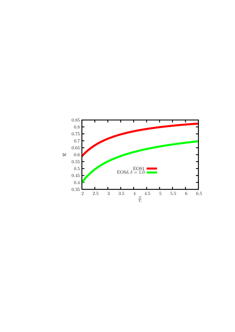
Figure 4: (Color online) Relative susceptibility, $g^{\prime}_{2}(z_{g})$ (see Eq. (18), for pure gauge theory plasma as a function of $T/T_{c}$ for EOS1 and EOS$\delta$ ($\delta=1$).

.

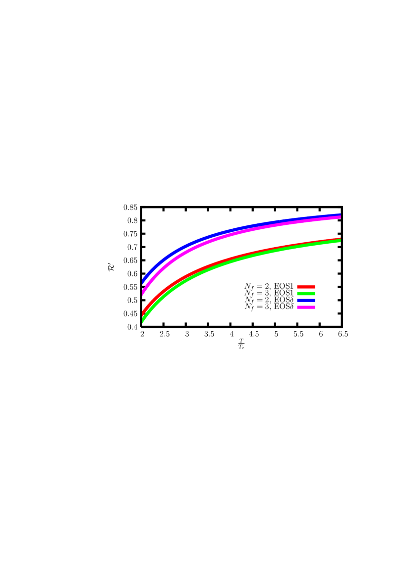
Figure 5: (Color online) Relative susceptibility, defined in Eq. (IV), for the full QCD plasma as a function of $T/T_{c}$, for EOS1 and EOS$\delta$ ($\delta=1)$. We have studied the cases $N_{f}=2,3$.

We see From Fig. 4 that the susceptibility of a purely gluonic plasma is weaker in the presence of interactions, approaching its ideal value asymptotically with increasing temperatures. Equivalently, there is a decrease in the value of the phenomenological coupling $Q^{2}$, relative to its ideal value.

The behavior of quark gluon plasma is not qualitatively different from that of a purely gluonic plasma, as may be seen from Fig.5. In other words, the quark contribution is of the same order as the purely gluonic contribution. However, the relative contribution from the quarks and the gluons does depend on the EOS considered. Indeed, with EOS1 (where interactions up to $O(g^{5})$ are included), Fig.6 shows that the quark contribution dominates slightly over the gluonic contribution for $N_{F}=2$. The dominance is more pronounced for the more realistic case $N_{F}=3$. In contrast, we see from Fig. 7, that EOS$\delta$ (with $\delta=1$) predicts that the gluonic contribution is marginally larger for $N_{F}=2$ and becomes sub dominant when $N_{F}=3$. This distinction between the two EOS is of no practical consequence since, given $T_{c}\sim 170MeV$, one has to necessarily work with $N_{F}=3$ at $T=2T_{c}$.

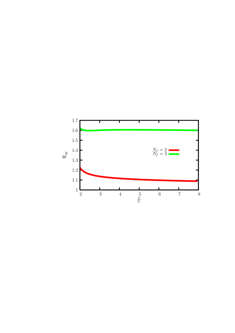
Figure 6: (Color online) Ratio of the quark to gluonic contributions to the susceptibility (see Eq.(19) as a function of $T/T_{c}$, as predicted by EOS1.

.

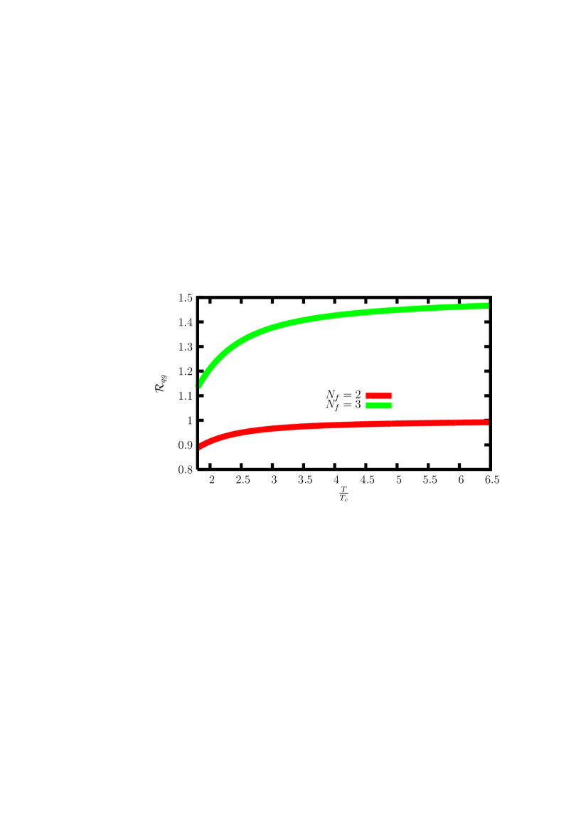
Figure 7: (Color online) Ratio of the quark to gluonic contributions to the susceptibility (see Eq.(19) as a function of $T/T_{c}$, for EOS$\delta$, $\delta=1$..

V The heavy quark potential

Now we shall apply the results of the previous sections to discuss the heavy quark potential in the presence of interacting medium. We consider the Cornell potential

$$\phi(r)=-\frac{\alpha}{r}+\Lambda r$$

where $\alpha$ and $\Lambda$ are phenomenological constants. The first term shows the Coulombic behavior and dominates at small distance while the second term causes linear confinement, dominating at large distances.

It had been expected earlier that the long range part of the Cornell potential does not survive in the quark gluon phase. This expectation assumes a phase transition from the hadronic to deconfined phase. More recent studiesphaseT indicate that in all likelihood, deconfinement is not a phase transition, but a crossover. If such to be the case, there is no reason to expect the linear part of the potential to disappear completely. With this in mind, we study the modifications of both the Coulomb and linear terms, and examine how reasonable the EOS under consideration are.

Since the potential has no explicit color dependence, it is sufficient to employ the Abelian components of the permittivities. At $\omega=0$, the quark and gluon permittivities have the form

$$\tilde{\epsilon}_{q}(k,T)=1+\frac{16\pi{Q^{2}}T^{2}}{k^{2}}f_{2}(z_{q})$$

$$\tilde{\epsilon}_{g}(k,T)=1+\frac{16\pi{Q^{2}}T^{2}}{k^{2}}g_{2}(z_{g}).$$

Therefore the full permittivity reads

$$\tilde{\epsilon}(k,T) = \frac{(\tilde{\epsilon}_{g}+\tilde{\epsilon}_{q})}{2}$$ (22)

$$= 1+\frac{8\pi^{2}{Q^{2}}T^{2}}{k^{2}}\bigg{[}N_{f}f_{2}(z_{q})+g_{2}(z_{g})\bigg{]}$$

$$\equiv 1+\frac{m_{D}^{2}}{k^{2}},$$

in terms of the Debye mass $m_{D}^{2}=8\pi Q^{2}T^{2}\big{[}N_{f}f_{2}(z_{q})+g_{2}(z_{g})\big{]}$.

The $q\bar{q}$ potential undergoes a modification due to the medium via $\tilde{\epsilon}(k,T)$, as given by $\tilde{\phi}(k)\rightarrow\tilde{\phi}(k)/\tilde{\epsilon}(k,T)\equiv\tilde{\phi}_{s}(k,T)$. We note that in determining the Fourier transform of Cornell potential, we regulate the linear term exactly the same way we regulate the Coulomb term, by multiplying with an exponential damping factor. The damping is switched off after the Fourier transform is evaluated. The Fourier transform is thus obtained as

$$\tilde{\phi}(k)=-\sqrt{\frac{2}{\pi}}\frac{1}{k^{2}}-\frac{4\Lambda}{k^{4}\sqrt{2\pi}}$$ (23)

The modified potential thus acquires the form

$$\tilde{\phi}_{s}(k,T)=-\sqrt{\frac{2}{\pi}}\frac{\alpha}{k^{2}+m^{2}_{D}}-\frac{4}{\sqrt{2\pi}}\frac{\Lambda}{k^{2}(k^{2}+m^{2}_{D})}.$$ (24)

We note that for a gluonic plasma, $m^{2}_{D}=16\pi Q^{2}T^{2}g_{2}(z_{g})$.

On comparing Eq.24 with Eq.23 we infer the renormalization of the couplings

$$\Lambda_{eff}=\frac{\Lambda}{1+\frac{m^{2}_{D}}{k^{2}}};~{}~{}\alpha_{eff}=\frac{\alpha}{1+\frac{m^{2}_{D}}{k^{2}}}.$$

V.1 Screening of the heavy quark potential

Of interest to us is the form of the potential in the real space, as a function of spatial separation. The inverse Fourier transform yields it to be

$$\phi_{s}(r,T) = (\frac{2\Lambda}{m^{2}_{D}}-\alpha)\frac{\exp{(-m_{D}r)}}{r}$$ (25)

$$- \frac{2\Lambda}{m^{2}_{D}r}+\frac{2\Lambda}{m_{D}}-\alpha m_{D}.$$

It follows from the above equation that the medium transforms the linear potential to the long range Coulomb form, just as it modifies the bare Coulomb term to the short ranged Yukawa.. The modified potential is not short ranged; it is not confining either. To appreciate this, note that at large $T$, the above expression reduces to

$$\phi_{s}(r,T)\sim-\frac{2\Lambda}{m^{2}_{D}r}-\alpha m_{D}$$ (26)

Thus, contrary to the Maxwellian plasmas which support only short range interactions, the two EOS predict that the heavy quark potential continues to be long ranged, although absolute confinement, which was a quintessential feature of the unscreened potential, is lost. It might as well be that the above results signify that the EOS fail to describe the hadronic matter in its deconfined state, On the other hand, since the transition from the hadronic to QGP phase could be a cross over, and not a phase transition phaseT , it could be possible that the above result is not entirely devoid of physical significance. If we adopt the latter view, if only for the purposes of analysis, a discussion of screening cannot, therefore rely entirely on the interpretation of inverse Debye mass as a screening length in its usual sense. We address the issue below .

Let us consider the high temperature limit of the potential, given by Eq.(26). Ignoring the additive contribution, the energy of the $q\bar{q}$ in the ground state is simply given by

$$E_{g}=\frac{m_{q}\Lambda^{2}}{m^{4}_{D}},$$

where $m_{q}$ is the mass of heavy quark.

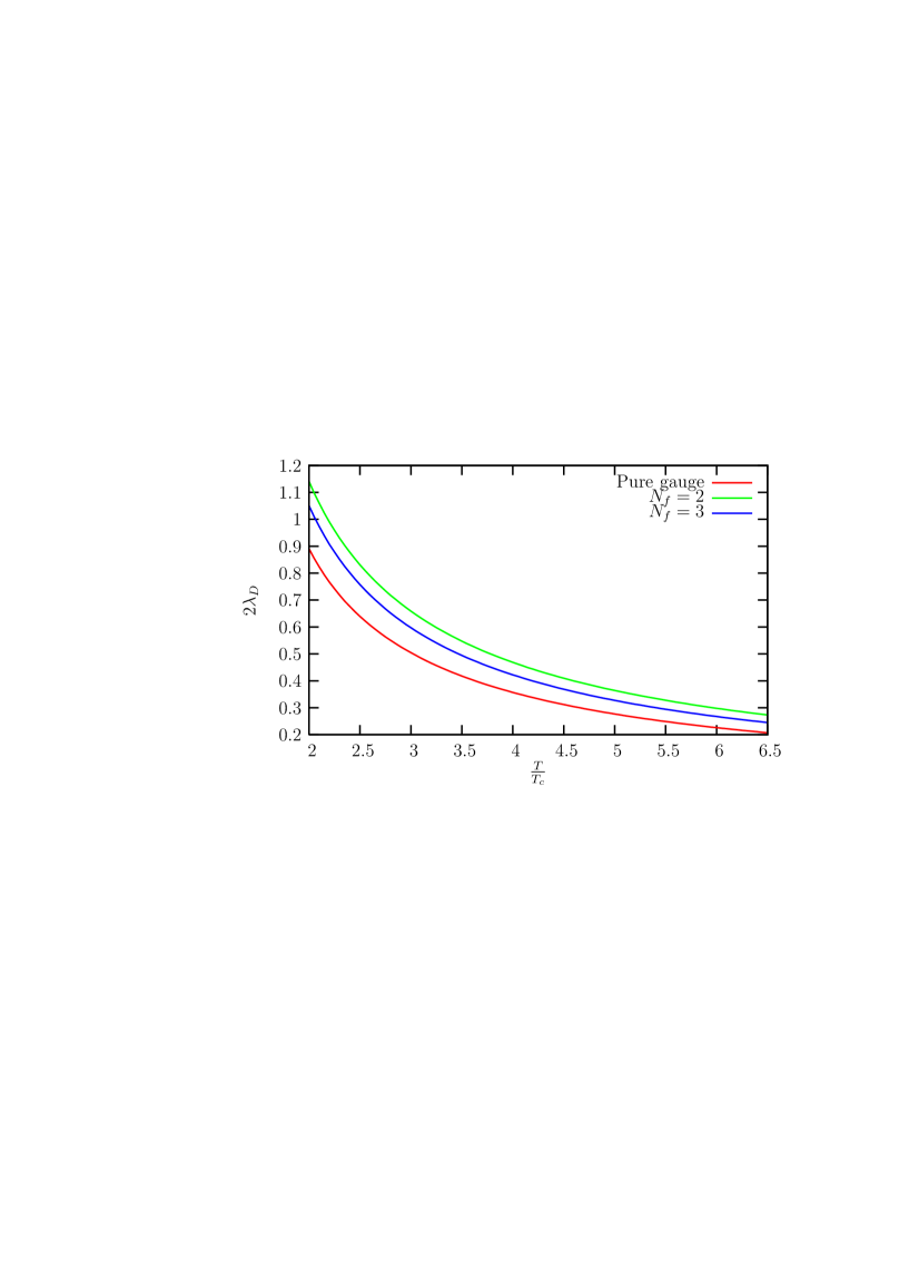
Figure 8: (Color online) Debye screening length for gluonic and quark-gluon plasmas as a function of $T/T_{c}$ for EOS1.

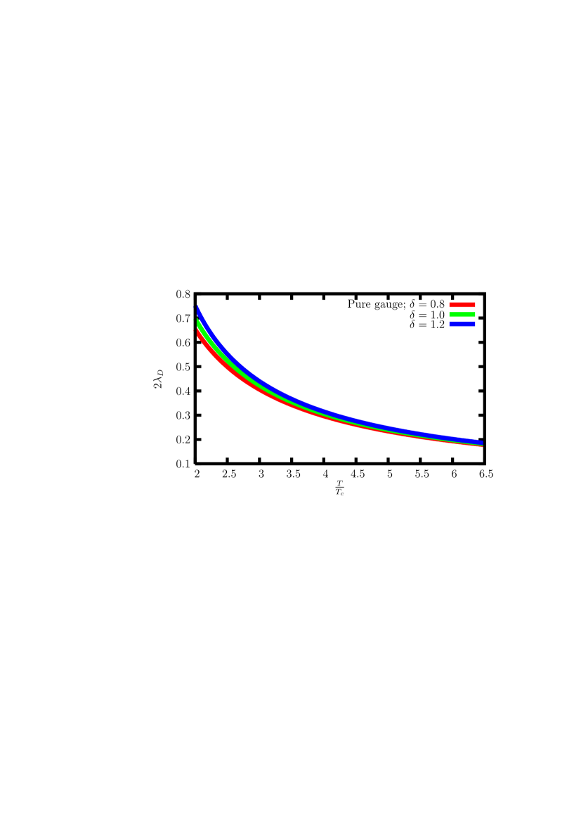
Figure 9: (Color online) Debye screening length for pure gauge theory plasma in EOS$\delta$ as a function of $T/T_{c}$ for various values of $\delta$.

The binding energy is, of course, temperature dependent and approaches zero as $T\rightarrow\infty$. At any finite temperature though, the quarks possess a thermal energy $E_{T}\sim T$ (by equipartition theorem), leading to an ionization of the quarkonium when $E_{T}$ matches the binding energy. The dissociation temperature $T_{d}$ is determined by the matching conditions. In the case of pure gauge theory,

$$\frac{m_{q}\Lambda^{2}}{384\pi^{2}Q^{4}T^{5}_{c}}=(\frac{T_{D}}{T_{c}})^{5}g^{2}_{2}(z_{g}).$$ (27)

And for full QCD:

$$\frac{m_{q}\Lambda^{2}}{384\pi^{2}Q^{4}T^{5}_{c}}=\frac{1}{4}(\frac{T_{D}}{T_{c}})^{5}\bigg{(}N_{f}f_{2}(z_{q})+g_{2}(z_{g})\bigg{)}^{2}$$ (28)

V.2 Estimation of $Q$ and a determination of the screening length

The above equation is still not amenable to comparison with experiments since it has the undetermined parameter $Q$. To estimate $Q$, we need an additional input which we obtain by comparing the screening length obtained as a solution of Eqs. (27) and (28) with the lattice results, reported by Kazmarek and Zantow zantow . Note that the screening lengths for gluonic and quark gluonic plasmas are respectively given by

$$\lambda^{g}_{D}=\frac{1}{QT}\frac{1}{\sqrt{\bigg{(}}16\pi g_{2}(z_{g})\bigg{)}},$$ (29)

$$\lambda_{D}=\frac{1}{QT}\frac{1}{\sqrt{\bigg{(}}8\pi(N_{f}f_{2}(z_{q})+g_{2}(z_{g}))\bigg{)}}.$$ (30)

Recalling that our results are valid for $T>2T_{c}$, we match the pure gauge theory result with the lattice values $\lambda\sim 0.15$ fm, and $T_{c}=0.27$ GeV. We obtain

$$\lambda^{g}_{D}=\frac{0.19}{0.27}\frac{1}{4Q(T/T_{c})}\frac{1}{\sqrt{(}\pi g_{2}(z_{g}))}.$$ (31)

This leads to the estimate $Q\sim 0.15$. The temperature dependence of the screening lengths can be thereafter determined for the two equations of state. We emphasize that the choice $\delta=0.9$ gives the best agreement between EOS$\delta$ and the lattice EOS for gluonic plasma fkarsch .

V.3 Dissociation temperatures for quarkonia

Since there are no free parameters left, it is a straight forward task to determine the dissociation temperatures for the heavy quark bound states. We are principally interested in $J/\Psi$ and $b\bar{b}$ states, for which we have gathered the results in Table. 1, after obtaining graphical solutions for Eq.(27) and Eq.(28). We have employed the values $m_{c}=1.5GeV,~{}m_{b}=4.5GeV$ and $\Lambda=0.18GeV^{2}$ for the quark masses and the strength of the Cornell potential. It is noteworthy that the dissociation temperatures are all roughly in the range $T_{D}\approx(2-3)T_{c}$, which is higher than the temperatures achieved so far. Since the temperatures expected at LHC is in the range $T\sim 2T_{c}-3T_{c}$, one may expect to test these predictions there.

We now turn our attention to compare hot QCD estimates for dissociation temperatures with other theoretical works. In a recent paper, Satzsatz has studied the dissociation of quarkonia states by studying their in-medium behavior. These estimates were based on the Schrödinger equation for Cornell potential. In a more recent work, Alberico et alprd75 reported the dissociation temperatures for charmonium and bottomonium states for $N_{f}=0$ and $N_{f}=2$ QCD. In this work, they have solved the Schrödinger equation for the charmonium and bottomonium states at finite temperature in the presence of temperature dependent potential– computed from the lattice QCD. We have quoted these results in Table 2. The estimates for $N_{f}=0$ and $N_{f}=2$ cases for both EOS1 and EOS$\delta$(Table 1) are closer to Ref.satz . On the other hand the estimates for $J/\Psi$ dissociation temperatures for both EOS1 and EOS2 are larger than that of Ref.prd75 while bottomonium dissociation temperature estimates are slightly smaller. We do not have lattice estimates at present to compare the dissociation temperatures for $N_{f}=3$ QCD. However the hot QCD estimates are consistent with the lattice predictionssdata on the survival of heavy quarkonia states near $2T_{c}$ and predictions of dynamical $N_{f}=2$ QCD by Aarts et algert . Along these results, we wish to mention the very recent estimates on dissociation temperature reported by Mócsy and Pétreeczkymoscky . Their estimates for $J/\Psi$ dissociation temperature is $1.2T_{c}$ and for $\Upsilon$ is $2T_{c}$. The estimates for both EOS1 and EOS$\delta$ are larger as compare to these results.

Table 1: The dissociation temperature($T_{D}$) for various quarkonia states (in unit of $T_{c}$).

Hot EOS	Quarkonium	Pure QCD	$N_{f}=2$	$N_{f}=3$
EOS1	$J/\Psi$	2.2	2.62	2.46
	$\Upsilon$	2.5	3.14	2.94
EOS$\delta$	$J/\Psi$	1.86	2.38	2.24
$\delta=0.8$	$\Upsilon$	2.12	2.76	2.58
EOS$\delta$	$J/\Psi$	1.95	2.45	2.32
$\delta=1.0$	$\Upsilon$	2.2	2.83	2.66
EOS$\delta$	$J/\Psi$	2.03	2.52	2.40
$\delta=1.2$	$\Upsilon$	2.28	2.9	2.74

Table 2: The dissociation temperature($T_{D}$) for various quarkonia states (in unit of $T_{c}$) from Ref.satz and Ref.prd75 . The first and third rows are the estimated values for dissociation temperature from Ref.satz and second and fourth are from Ref.prd75

Quarkonium	$N_{f}$=0	$N_{f}=2$
$J/\Psi$	2.1	$>$2
$J/\Psi$	1.40	1.45
$\Upsilon$	$>$2
$\Upsilon$	2.96	3.9

V.3.1 Comparison of Debye screening length with lattice results

Finally, with a view to benchmark our estimates of the screening lengths, by comparing them with the recent lattice results reported by Kazmarek and Zantow zantow , we plot $2\lambda_{D}$ as a function of $T/T_{c}$. The results are shown for EOS1 as well as EOS$\delta$, for three values $\delta=0.8,1.0,1.2$. The results for pure gauge theory (gluonic plasma) are shown in Fig.9, and Fig.10 shows the results for full QCD. We find that on comparison with Fig.2 of Ref. zantow , these values, $\delta\sim 1$ are the most favored which justifies, a posteriori our choice for the parameter.

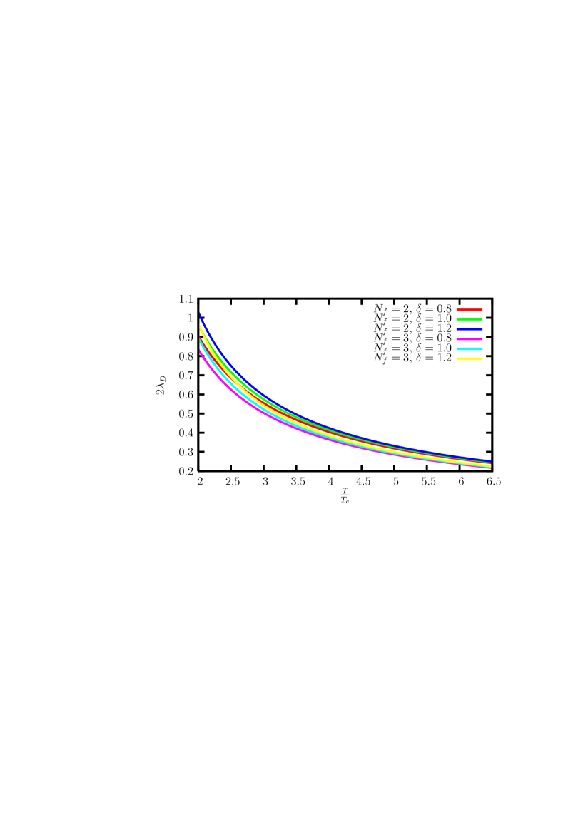
Figure 10: (Color online) Debye screening length for full QCD plasma as predicted by EOS$\delta$ as a function of $T/T_{c}$ for various of $\delta$.

VI Conclusions and Outlook

In conclusion, we have successfully extracted the quasi-free particle content of two hot QCD equations of states and used them to determine the chromo-electric permittivities within the standard Boltzmann-Vlasov kinetic approach. The Abelian and the non-Abelian components of the permittivity are obtained, for pure gauge theory and the full QCD. We have shown that the effect of the interactions is to merely renormalize the magnitude of the effective color charge, $Q$. We have used the permittivities to study critically the modifications in a realistic heavy quark potential. The dissociation temperatures are carefully estimated, by fixing the magnitude of $Q$ by an explicit matching with a lattice result. The values obtained are quite close to the exact lattice results. The viability of the two EOS, especially EOS$\delta$ is thus phenomenologically well supported. Our analysis suggests strongly, and in agreement with the lattice results, that $J/\Psi$ suppression can be seen in QGP only for $T\geq 3T_{c}$.

A true test of the above predictions would be possible if we succeed in extracting a quasi particle description from the lattice EOS. Studies are under way in this direction. It should also be of interest to extend the analysis to other signatures like strangeness enhancement, and also for QGP with a finite baryonic chemical potential avrn ; ipp . These will be taken up in a later work.

Acknowledgments: VC acknowledges Anton Rebhan for useful comments and suggestions on the work in the present manuscript during Les Houches QCD school– Hadronic collisions at the LHC and QCD at high density at Centre de Physique des Houches, France - Mar 25 - Apr 4, 2008. VC also acknowledges C.S.I.R., New Delhi (India) for the financial support.

References

-
(1)
PHENIX Collaboration, Nucl. Phys. A 757 (2005) 184;
PHOBOS Collaboration , Nucl. Phys. A 757 (2005) 28;
BRAHMS Collaboration , Nucl. Phys. A 757 (2005) 01;
nucl-th/0308024. - (2) STAR collaboration, J. Adams et al. Nucl. Phys. A 757 (2005) 102.
- (3) M. J. Tannenbaum, Rept. Prog. Phys. 69 (2006) 2005.
-
(4)
Itzhak Tserruya,
Nucl. Phys. A 774 (2006) 415;
Nucl. Phys. A 774 (2006) 433 . - (5) Patricia Fachini, AIP Conf. Proc. 857 (2006) 62 .
- (6) Steffan A. Bass, Pramana 60 (2003) 593.
- (7) T. Csörgö, S. Hegyl, T. Novak̀ and W. A. Zajc, Acta Phys. Polon. B 36 (2005) 329 .
- (8) Frithjof Karsch, Nucl. Phys. A 698 199(2002).
- (9) Y. Aoki, Z. Fodor, S. D. Katz and K. K. Szabo, JHEP 0601 (2006) 089.
- (10) P. Kovtun, D. T. Son, A. O. Starinets, Phys. Rev. Lett. 94 (2005) 111601.
- (11) E. V. Shuryak, Nucl.Phys. A 774 (2006) 387.
- (12) R. Baier and P. Romatschke, nucl-th/0610108.
- (13) H. J. Drescher, A. Dumitru, C. Gombeaud and J. Y. Ollitrault, arXiv:0704.3553 [nucl-th].
- (14) Akhilesh Ranjan and V. Ravishankar, arXiv:0707.3697 [nucl-th].
- (15) S. Haung and M. Lissia, Nucl. Phys. B438 (1995) 54.
- (16) Daniel F. Litim and Cristina Manuel, Phys. Rep. 364 (2002) 451.
- (17) T. Matsui and H. Satz, Phys. Lett. B 178 (1986) 416.
- (18) H. T. Elze and U. Heinz, Phys. Rep. 183 (1989) 81.
- (19) Gouranga C Nayak and V. Ravishankar, Phys. Rev. D 55 (1997) 6877; Phys. Rev. C 58 (1998) 356.
- (20) R. S. Bhalerao and V. Ravishankar, Phys. Lett. B 409 (1997) 38; Ambar Jain and V.Ravishankar, Phys. Rev. Lett. 91 (2003) 112301.
- (21) I. Zahed and E. V. Shuryak, Phys. Rev. C 74 (2006) 044908; ibid (2006) 044909 .
- (22) C. M. Hung and E. V. Shuryak, Phys. Rev C 57 (1998) 4.
- (23) Jean- Paul Blaizot and Edmond Iancu, Physics Reports 359 (2002) 355.
- (24) Ulrich Heinz, Proceedings of *Swansea 2005, Extreme QCD* 3-12.
- (25) R. D. Pisarski, Phys. Rev. Lett. 63 (1989) 1129.
- (26) E. Braaten and R. D. Pisarski, Nucl. Phys. B 337 (1990) 569.
- (27) E. Braaten and R. D. Pisarski, Nucl. Phys. B 339 (1990) 310. See also
- (28) R. Jackiw and V. P. Nair, Phys. Rev. D 48 (1993) 4991.
- (29) Jean-Paul Blaizot and Edmond Iancu, Phys. Rev. Lett. 70 (1993) 3376.
- (30) J. P. Blaizot and E. Iancu, Nucl. Phys. B 417 (1994) 608.
- (31) J. P. Blaizot and E. Iancu, Phys. Rev. Lett. 72 (1994) 3317.
- (32) J. P. Blaizot and E. Iancu, Nucl. Phys. B 421 (1994) 565.
- (33) P.F. Kelly, Q. Liu, C. Lucchesi, C. Manuel, Phys. Rev. Lett . 72 (1994) 3461.
- (34) P.F. Kelly, Q. Liu, C. Lucchesi, C. Manuel, Phys. Rev D 50 (1994) 4209. For a comprehensive review see
- (35) Daniel F. Litim and Cristina Manuel, Phys. Rep. 364 (2002) 451.
- (36) E. Eichten, K Gottfried, T. Kinoshita, K. D. Lane and T. M. Yan, Phys. Rev. D 21 (1980) 203 .
- (37) F. Karsch, hep-lat/0601013; Journal of Physics: Conference Series 46 (2006) 121; O. Philipsen, Pos(LAT 2005) 016; Urs M. Heller, Pos(LAt 2006) 011(hep-lat/0610114); M. A. Stephanov, Pos(LAT 2006) 024; Cheng et al, arXiv:0710.0354.
-
(38)
P. Arnold and Chengxing Zhai,
Phys. Rev. D 50 (1994) 7603;
Phys. Rev. D 51 (1995) 1906. - (39) Chengxing Zhai and B. Kastening, Phys. Rev. D 52 (1995) 7232.
- (40) Please see Fig.13 of this Ref.; Frithjof Karsch, Lect. Notes Phys. 583 (2002) 209 (arXiv:hep-lat/0106019).
- (41) Vinod Chandra, Ravindra Kumar and V. Ravishankar, Phys. Rev. C 76 (2007) 054909 (arXiv:0705.0962 [nucl-th]).
- (42) K. Kajantie, M. Laine, K. Rummukainen and Y. Schroder, Phys. Rev. D 67 (2003) 105008.
- (43) Rudolf Baier and Krzysztof Redlich, Phys. Rev. Lett. 84 (2002) 2100.
-
(44)
G. Boyd, J. Engels, F. Karsch, E. Laermann,
C. Legeland, M. Luetgemeier, B. Petersson,
Nucl. Phys. B469 (1996) 419; Phys. Rev. Lett. 75 (1995) 4169. - (45) J.-P. Blaizot, E. Iancu, A. Rebhan, Phys. Rev. D 68 (2003) 025011.
- (46) J.-P. Blaizot, E. Iancu, A. Rebhan, Phys. Rev. Lett. 83 (1999) 2906; Phys. Rev. D 63 (2001) 065003; Phys. Lett. B 470 (1999) 181.
- (47) O. Kazmarek and F. Zantow, Pos (LAT 2005) 177(arXiv:hep-lat/0510093).
- (48) Helmut Satz, Nucl. Phys. A 783 (2007) 249.
- (49) W. M. Alberico, A. Beraudo, A. De Pace and A. Molinari, Phys. Rev. D 75 (2007) 074009.
- (50) O. Kaczmarek, F. Karsch, P. Petreczky and F. Zantow, Phys. Lett. B453 (2002) 41, Phys. Rev. D70 (2004) 074505, A. Moesky, arXiv:hep-ph/0609204; F. Karsch, Nucl. Phys. A783 (2007) 13; T. Umeda and H. Matsufuru hep-lat/0501002; O. Kaczmarek and F. Zantow, Phys. Rev. D71 (2005) 114510; S. Datta, F. Karsch, P. Petreczky and I. Wetzorke, Phys.Rev. D 69 (2004) 094507; M. Asakawa and H. Hatsuda, Phys. Rev. Lett.92 (2004) 012001.
- (51) Gert Aarts, Chris Allton, Mehmet Bugrahan Oktay, Mike Peardon, Jon-Ivar Skullerud, Phys. Rev. D 76, 094513 (2007).
- (52) A. Mócsy and Péter Petreczky, Phys. Rev. Lett. 99 (2007) 211602 (arxiv:0706.2183[hep=ph]).
- (53) A Vuorinen, Phys. Rev. D 68 (2003) 054017.
- (54) A. Ipp, K. Kajantie, A. Rebhan and A. Vuorinen, Phys. Rev. D 74 (2006) 045016.