X-Ray Propagation in Tapered Waveguides: Simulation and Optimization

Abstract

We use the parabolic wave equation to study the propagation of x-rays in tapered waveguides by numercial simulation and optimization. The goal of the study is to elucidate how beam concentration can be best achieved in x-ray optical nanostructures. Such optimized waveguides can e.g. be used to investigate single biomolecules. Here, we compare tapering geometries, which can be parametrized by linear and third-order (Bézier-type) functions and can be fabricated using standard e-beam litography units. These geometries can be described in two and four-dimensional parameter spaces, respectively. In both geometries, we observe a rugged structure of the optimization problem’s “gain landscape”. Thus, the optimization of x-ray nanostructures in general will be a highly nontrivial optimization problem.

, and

1 Introduction

X-ray waveguides are promising novel optical devices to generate x-ray quasi-point sources for hard x-ray imaging [1, 2]. X-ray waveguides (WG) have been designed and fabricated as planar layered systems (1D-WG) [3, 4, 5] or as lithographic channels (2D-WG) [6, 7]. In both cases (guiding layer or guiding channel) mainly waveguides with a core of constant cross section have been considered. Beam propagation in such structures, which are translationally invariant along the propagation axis $z$, is by now well studied and understood [8, 9, 10, 11]. As optical elements, such waveguides serve mainly two purposes: Firstly, the radiation modes are damped out and the cross section of the exit beam is thus reduced significantly with respect to the incident beam. Secondly, in the case of single-mode waveguides [12], the phase and amplitude of the wave is determined exactly, and therfore presents an ideal wave for coherent imaging. In other words, the waveguide acts as a spatial and coherence filter, but not to collimate or to concentrate the beam. The flux density necessary for nanometer-sized beam with high enough intensities for practical applications must then be achieved by focusing elements placed in front of the waveguide, such as Kirkpatrik-Baez (KB) mirrors [13, 7], Fresnel zone plates [14] or compound refractive lenses [15, 16].

Here we address the question to which extent tapering of the waveguide can be used to concentrate the beam and to filter it at the same time. This would make pre-focusing optics in front of the waveguide obsolete for some applications. A first experimental realization was demonstrated by tapered air-gap waveguides [17], but was restricted to the multi-modal regime. Bergemann et al. have then studied linearly tapered x-ray waveguides by analytical and numerical calculation [18], concentrating on minimum beam width at the exit. Here we want to generalize the numerical studies to non-linear tapering profiles. Rather than the minimum achievable beam width, which has been addressed before [18], we address the maximum flux density enhancement as function of tapering parameters, and the associated question of an optimum interface geometry. As in all problems of reflective optics, e.g.  bent mirrors, one would assume that the shape function is a crucial parameter in the problem. As a first step, we consider both linear and third order polynominal interface geometries. Note that the parameters studied correspond well to structures which can also be fabricated by e-beam lithography. The propagation in the stuctures is studied by numerical solution of the parabolic wave equation (PWE), as used previously for standard waveguides [19, 10]. The use of the PWE will be briefly explained in the next section, followed by the simulation results.

2 The simulation method

The propagation of monochromatic x-rays in materials is described by the Helmholtz equation

$$[\triangle+k^{2}n^{2}]\Psi=0~{}.$$ (1)

$\Psi$ denotes an electric field component in this scalar wave equation, $k=\frac{2\pi}{\lambda}$ the wavenumber, and $\lambda$ the wavelength. The index of refraction is given by $n=1-\delta-\mathrm{i}\beta$, where the imaginary part accounts for absorption. The Laplacian is written as $\triangle=(\partial_{x}^{2}+\partial_{z}^{2})$ for the two-dimensional case which is of interest here. The direct solution of this elliptical differential equation is problematic due to numerical instability and the fact that the region of interest is large compared to the wavelength (micrometers up to millimeters compared to Ångström). A numerically much more stable alternative is provided by the parabolic wave equation, which can be used in controlled and excellent approximation for forward propagation problems in the x-ray regime [20, 21, 22]. To this end, a function $u(x,z)$ is defined by $\Psi(x,z)=:u(x,z)\exp(-\mathrm{i}kz)$. Neglecting terms of order $\mathcal{O}(\partial_{z}^{2}u)$ which is justified if the $z$-axis is almost parallel to the wavevector, the Helmholtz equation is fullfilled for $\Psi$, under the condition that $u$ solves the parabolic wave equation

$$[-2\mathrm{i}k\partial_{z}+\partial^{2}_{x}+k^{2}(n^{2}-1)]u=0$$ (2)

Mathematically, this equation is of the same form as the stationary Schrödinger equation for a massive particle (without spin) in a potential. After renaming of variables, the potential in the Schrödinger equation is equivalent to the the refraction index $n$ profile in the optical case considered here.

In order to simplify the expressions and to find a suitable length scale for numerical calculations, we use the natural units $\frac{1}{\delta k}$ for the distance along the propagation direction, and $W=\frac{\pi}{k\sqrt{2\delta}}$ for the lateral dimension, respectively. Note that $W$ is the critical width at which a waveguide becomes mono-modal, i.e. the width at which the waveguide supports only a single mode [18, 23]. At the same time, a waveguide of width $d=W$ leads to the highest possible wave confinement. The intensity distribution of the wave broadens both for smaller and larger $d$. While the second case is trivial, it is important to note that the nearfield intensity distribution is broadened by evanescent waves in the cladding, if $d$ is reduced below $W$. Using these natural units

$$Z:=\delta kz,\qquad X:=\frac{x}{W}~{},$$ (3)

(2) can be rewritten as

$$\partial_{Z}u=-\frac{\mathrm{i}}{\pi^{2}}\partial_{X}^{2}u+\left\{\begin{array}[]{ll}(i-\frac{\beta}{\delta})u,&\quad\text{in material}\\ 0,&\quad\text{in vacuum}.\end{array}\right.$$ (4)

The ratio $\frac{\beta}{\delta}$ remains the only material dependent parameter in this equation.

The equation is solved using a Crank-Nicolson finite-difference scheme, which was already proved to give reliable results for x-ray waveguides and Fresnel zone plates [22, 24]. For the initial values, a plane wave propagating along $z$ was assumed. The lateral boundary conditions are given by a damped plane wave propagating in the material far away from the region of interest.

For field propagation in vacuum, the Fresnel-Kirchhoff integral for two-dimensional beam propagation [25] was used [26],

$$\Psi(x,z)=\frac{\mathrm{i}}{\sqrt{\lambda}}\int\mathrm{d}x^{\prime}\Psi(x^{\prime},0)\frac{\mathrm{e}^{-\mathrm{i}kr}}{\sqrt{r}}\cos\alpha~{},$$ (5)

where $\alpha$ is the angle between the $z$-axis and the vector $(x-x^{\prime},z)$. The corresponding distance to the origin is $r^{2}=z^{2}+(x-x^{\prime})^{2}$.

3 Tapered x-ray waveguides: shape optimization

We have considered two generic types of tapering geometry: (i) the linear taper, and (ii) a tapering function parameterized by Bézier curves. For comparison with experimental values, we have chosen material parameters and photon energy $E$ according to recent experiments and present fabrication methods. Vaccuum channels in $Si$ have been simulated at a photon energy $E=12\,\mathrm{keV}$. Taking air/vaccuum as the guiding material simplifies simulations because only the index of refraction of the cladding differs from unity. Optically, the structures are still very close to the experiments with polymer channels in $Si$ [7, 27], and are completely equivalent to the second generation of x-ray waveguide channels fabricated by e-beam lithography, ion etching and subsequent wafer bonding of a cap wafer. For both tapering geometries, the waveguide end width was held constant at $d=1,\,W=20\,\mathrm{nm}$ which is the critical width $W=\frac{\pi}{k\sqrt{2\delta}}$ for single-mode waveguides [18, 23]. At this value, the resolution limit of waveguides is reached, corresponding to a full width at half maximum $\mathrm{FWHM}_{\mathrm{min}}=0.64\,W$ for the intensity profile in the channel of width $W$ [18].

The goal of the optimization was to quantify the field propagation and confinement, for given opening width $D$ and end width $d$ or for given $d$ only. In general, one can expect that optimization of x-ray nanostructures might be highly non-trivial, as for many optimization problems occurring in physics [28, 29]. Nevertheless, since we restricted ourself here to the two above mentioned tapering geometries, we could use a quite simple optimization algorithm, see below. The two tapering geometries were parameterized as follows (see Fig. 1):

• In the linear case, a straight interface seperates the channel from the cladding at an opening angle $\vartheta$. The length of the waveguide is denoted by $L$.

• In the case of a Bézier curve interface, the shape is controlled by two vectors $\mathbf{P}_{1}=(x1,y1)$ and $\mathbf{P}_{2}=(x2,y2)$, which determine the derivative of the curve at the endpoints and thereby fully define a curve of third polynomial degree [30].

We have used these functions also because they can be handled by pattern generators of modern e-beam lithography units.

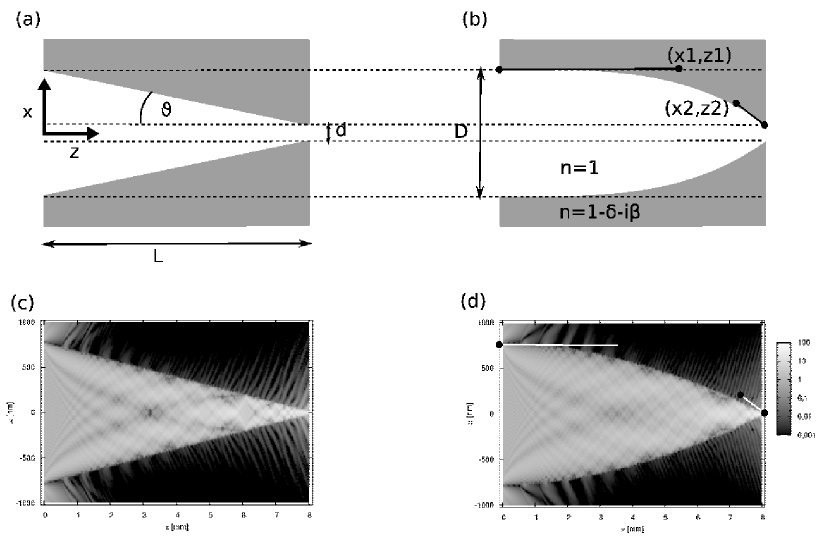
Figure 1: Shape functions and field distribution of taperd waveguides: the top row shows the schematics, the bottom row the calculated intensity distribution for the optimal parameters of each kind. The waveguides consists of vacuum channels embedded in Silicon at a photon energy of $E=12\,\mathrm{keV}$. (bottom left) Linear taper with an opening angle $\vartheta=0.037\,\vartheta_{c}$, transporting radiation collected within a width of $D=0.77\mu$m over a propagation distance of $L=8\,\mathrm{mm}$ down to the critical exit cross section of $d=19.88\,\mathrm{nm}$, corresponding to the critical width $W$ of $Si$. (bottom right) Waveguide tapered with a Béziercurve interface. The lengths $d$, $D$ and $\ell$ as above. The two control vectors are $P_{1}=(x_{1}=3.45\,\mathrm{mm},y_{1}=766.2\,\mathrm{nm})$ and $P_{2}=(x_{2}=7.25\,\mathrm{mm},y_{2}=176.7\,\mathrm{nm})$, respectively

Firstly, let us consider the linear taper. Waveguides with linear taper have been simulated for different length $L$ and angle $\vartheta$. Fig. 2 shows the resulting peak intensities $I$ normalized to the incident intensity $I_{0}$, i.e. the gain $I/I_{0}$, at the end of the waveguide (exit plane) as a function of $L$ and $\vartheta$. Hence, this plot displays the “gain landscape” of the optimization problem. Even for this two-parameter space, a very rugged gain landscape is visible: With increasing opening width $D\simeq 2L\tan(\vartheta)$, $I$ first increases, in proportion to the geometric acceptance. The initial increase of $I(\vartheta,L={\rm const})$ crosses over to a surprisingly broad range of angles where the radiation transport and collimation raimains high, but is modulated by an oscillation occuring with a periodicity at which small. Finally, the intensity decreases when $\vartheta$ becomes too large, leading to a leaking of the intensity out of the confining interfaces. This leakage occurs for multireflections of high order $n$. The condition to prevent the leakage is simply given by $n\vartheta\leq\vartheta_{c}$, where $\vartheta_{c}$ is the angle of total reflection, as expected from ray optics. Nevertheless, at the end of the waveguide a dicrete set of rod-like intensity spikes are observed in the simulation, travering or ’leaking’ from the interface, see again Fig. 1. These rods or spikes originate from interference effects which would correspond to transmitted beams after multiple reflections in the ray-optical description. When $\vartheta$ is varied, these rods move and give rise to an oscillatory behavior in the exit plane. This effect is characterized by the oscillation between either sharp and intense profile at the exit, i. e. high $I$ and small with (full width at half intensity FWHM) or a smeared profile with low $I$ and large FWHM. In summary, $I(\vartheta,L={\rm const})$ possesses an optimum angle $\vartheta$, while $I(\vartheta={\rm const},L)$ increases with the length $L$, if $\vartheta$ is chosen accordingly, at least over the simulated range in $L$. We chose $L=8\,\mathrm{mm}$ as an experimentally achievable upper limit, see Fig. 2. For this length, the optimal angle is $\vartheta\simeq 0.037\vartheta_{c}$ leading to an opening width of $D=0.77\mu$m and $I/I_{0}=51.4$.

Figure 2: (top) Maximum intensity $I(\vartheta,L)$ at the exit normalized to the incident intensity $I_{0}$, as a function of opening angle $\vartheta$ and waveguide length $L$ for linear taper. (bottom) Maximum intensity $I(\vartheta,L=8{\rm mm})$ (left axis) and beam width FWHM (right axis) at the waveguide exit, as a function of $\vartheta$. The oscillations are phase shifted with respect to each other.

Now let us consider tapering of the Bézier type. Obviously, more parameters are needed to describe the space of Bézier curves which includes the linear as well as the parabolic case. Correspondingly, an optimization of the parameters is needed, since the optimum can no longer be found ’by eye’ from running a set of simulations. As a first step to a complete optimization, we optimized curves by simulating waveguides for different $y_{1}$ and $y_{2}$ at fixed $x_{1}=\frac{1}{3}L$ and $x_{2}=\frac{2}{3}L$. As in the linear case the exit was set to the critical width $d=W$. $D$ and $L$ were kept constant.

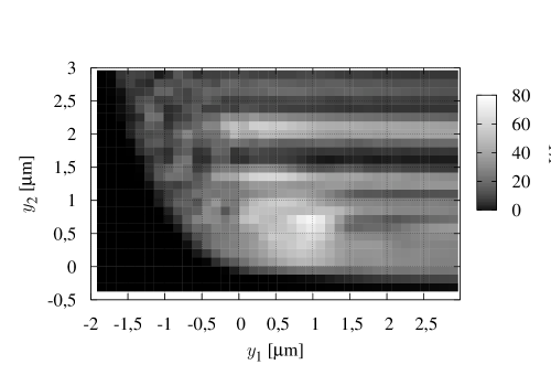
Figure 3: Maximum intensity $I$ (normalized by $I_{0}$) of a waveguide with Bézier-type tapering parameterized by $P_{1}=(1/3L,y_{1})$ und $P_{2}=(2/3L,y_{2})$. The function $I(y_{1},y_{2})$ exhibits a well pronounced global maximum.

The results, see Fig. 3 showed again a rugged gain landscape with a couple of local minima. Nevertheless, the maximum intensity seems to occur close to the linear case, and a few local minima are present in this particular region. Therefore, a simple approach was feasible: using the amoebae algorithm [31], the optimum parameters $P_{1}$, $P_{2}$ were searched, starting from the solution of the linear case $P_{1}=(\frac{1}{3}L,\frac{D}{2}-\frac{1}{3}A)$ and $P_{2}=(\frac{2}{3}L,\frac{D}{2}-\frac{2}{3}A)$ with $A=\frac{1}{2}(D-d)$. Note that using other starting values, the algorithm also found different local maxima, proving the complexity of the underlying gain landscape and the usefullness of our pre-scanning of the parameter space. As expected, the maximum intensity is higher for the more general Bézier case than for the linear taper, namely $82.2$ versus $51.4$ for the peak gain $I/I_{0}$, and $F=72.24$ versus $63.27$ for the integrated flux, see Tab. 1. However, this difference is surprisingly small. The result are tabulated in Tab. 1, showing maximum intensity $F$, integrated flux $J=\int\mathrm{d}xI$, width $w$ (FWHM) of intensity in the exit plane, as well as the angular acceptance on the incidence side, defined as the width (FWHM) of $I(\alpha)$, where $\alpha$ is the incidence angle $\alpha$. Note that if not otherwise stated, the angle $\alpha$ between incident beam and waguide axis was kept constant at $\alpha=0$. In addition to the two tapering geometries, the planar waveguide is included as a reference. As expected, the angular acceptance $\omega$ is much smaller for the tapered waveguides due to conservation of photon density in phase space (brilliance).

Table 1: Simulation results: maximum intensity $F$, flux $J$, width (FWHM) of intensity at the exit $w$, and FWHM for the angular dependency of the intensity (angular acceptance) $\omega$ are tabulated for (a) the plane, (b) linear tapered and (c) a waveguide with interfaces parameterized as Bézier curves (values obtained after parameter optimization).

	(a) planar	(b) linear	(c) Bézier
intensity $\frac{I}{I_{0}}$	$11,1\cdot 10^{-3}$	$51.4$	$82,2$
flux $\frac{J}{I_{0}d}$	$10,4\cdot 10^{-3}$	63,27	72,24
beam width $w$	15,2	17,8	12,0
angular acceptance $\frac{\omega}{\vartheta_{c}}$	0,929	0,031	0,025

4 Summary and Conclusion

We have studied beam propagation and concentation in tapered x-ray waveguides by simulations of finite-difference equations and subsequent parameter screening and optimization. The local slope of the waveguide interfaces and the associated tapering geometry is limited by the angle of total reflection, which restricts the tapering geometry to very elongated shapes. Over a device length on the order of $10$mm, an incoming beam with a width of $0.5-1\mu$m can be concentrated to the minimum width (FWHM) $w=0.65W\simeq 13\,\mathrm{nm}$ for silicon. The associated expected flux enhancement in the range of $40-80$ for one-dimensional focusing is observed in the simulation, confirming that most of the radiation is indeed transported to the exit aperture. For two-dimensional focusing, the gain would be squared, and would thus range up to about $5\times 10^{3}$, if $10$mm long structures are available. Note that both lithographic wafer processing and hollow glass fibers with well controlled shapes are conceivable even on length scales of $100$mm. However, let us stay withing a more conservative estimate based on a $10$mm long waveguide. As a result, the flux density gain, the size of the entrance aperture, and the angular acceptance $\omega$ are fully compatible with an optical scheme, where a synchrotron source is imaged by a lense of moderate numerical aperture (mirror system or CRL) onto the entrance aperture of a tapered waveguide. Let us consider realistic values for 3rd generation synchrotron sources: a source on the order of $100\mu$m cross section is demagnified by CRL or KB optics of focal length $f\simeq 1-5$m positioned $100$m behind the source. In this case, the focal spot and the convergence angle of the prefocussing optics can be matched to the entrance aperture and the angular acceptance $\omega$ of the tapered waveguide, respectively. In this case the combined gain of the pre-focussing optics and the tapered waveguide would lead to an intense and collimated virtual source, which is unlikely to be achieved by a single optical device. Most importantly, the simulation results show that the performance of the tapered waveguide does not depend on the shape function in a very sensitive way. Indeed, the beam can be funneled to the exit aperture surprisingly well already with a linear taper. In sharp contrast to single bounce mirror optics, the tapered waveguide almost forces the convergence of the beam, and is thus much less sensitive to figure errors. Nevertheless, we have also observed a rather rugged gain landspace for this optimization problem. Since the optimization was only for a few-parameter space, a simple algorithm could be used here. We expect that for the optimization of more complex x-ray nanostructures, like layered materials, more sophisticated algorithms have to be applied.

References

- [1] S. D. F. W. Jark, S. Lagomarsino, C. Giannini, L. D. Caro, A. Cedola, M. Müller, Non-destructive determination of local strain with 100-nanometre spatial resolution, Nature 403 (2000) 638–640.
-
[2]
C. Fuhse, C. Ollinger, T. Salditt, Waveguide-based off-axis holography with
hard x rays, Physical Review Letters 97 (25) (2006) 254801.
URL http://link.aps.org/abstract/PRL/v97/e254801 - [3] E. Spiller, A. Segmüller, Propagation of x rays in waveguides, Appl.Phys.Lett. 24 (1973) 60–61.
- [4] Y. P. Feng, S. K. Sinha, H. W. Deckman, J. B. Hastings, D. P. Siddons, X-ray flux enhancement in thin-film waveguides using resonant beam couplers, Phys. Rev. Lett. 71 (1993) 537–540.
- [5] W. Jark, A. Cedola, S. D. Fonzo, M. Fiordelisi, S. Lagomarsino, N. V. Kovalenko, V. A. Chernov, High gain beam compression in new-generation thin-film x-ray waveguides, Appl.Phys.Lett. 78 (2001) 1192–1194.
- [6] F. Pfeiffer, C. David, M. Burghammer, C. Riekel, T. Salditt, Two-dimensional x-ray waveguides and point sources, Science 297 (2002) 230–234.
- [7] A. Jarre, C. Fuhse, C. Ollinger, J. Seeger, R. Tucoulou, T. Salditt, Two-dimensional hard x-ray beam compression by combined focusing and waveguide optics, Phys. Rev. Lett. 94 (2005) 074801.
- [8] M. J. Zwanenburg, J. F. Peters, J. H. H. Bongaerts, S. A. de Vries, D. L. Abernathy, J. F. van der Veen, Coherent propagation of x rays in a planar waveguide with a tunable air gap, Phys. Rev. Lett. 82 (1999) 1696–1699.
- [9] L. D. Caro, C. Giannini, S. D. Fonzo, W. Yark, A. Cedola, S. Lagomarsino, Spatial coherence of x-ray planar waveguide exiting radiation, Optics Commun. 217 (2003) 31–45.
-
[10]
C. Fuhse, T. Salditt, Finite-difference field calculations for
two-dimensionally confined x-ray waveguides, Appl. Opt. 45 (19) (2006)
4603–4608.
URL http://ao.osa.org/abstract.cfm?URI=ao-45-19-4603 - [11] C. Fuhse, T. Salditt, Propagation of x-rays in ultra-narrow slits, Opt.Comm. 265 (2006) 140–146.
- [12] C. Fuhse, A. Jarre, C. Ollinger, J. Seeger, T. Salditt, R. Tucoulou, Front-coupling of a pre-focused x-ray beam into a mono-modal planar waveguide, Appl.Phys.Lett. 85 (2004) 1907–1909.
- [13] P. Kirkpatrick, A. V. Baez, Formation of optical images by x-rays, J. Opt. Soc. Am. 38 (1948) 766–774.
- [14] W. Chao, B. D. Harteneck, J. A. Liddle, E. H. Anderson, D. T. Attwood, Nature.
- [15] B. Lengeler, C. G. Schroer, M. Kuhlmann, B. Benner, T. F. Günzler, O. Kurapova, F. Zontone, A. Snigirev, I. Snigireva, Refractive x-ray lenses, J. Phys. D (38) (2005) A218–A222.
- [16] C. G. Schroer, B. Lengeler, Focussing hard x rays to nanometer dimensions by adiabatically focussing lenses, Phys. Rev. Lett. (94).
- [17] M. J. Zwanenburg, J. H. H. Bongaerts, J. F. Peters, D. Riese, J. F. van der Veen, Focusing of coherent x-rays in a tapered planar waveguide, Physica B 283 (2000) 285–288.
- [18] C. Bergemann, H. Keymeulen, J. F. van der Veen, Focusing x-ray beams to nanometer dimensions, Phys. Rev. Lett. 91 (2003) 204801.
- [19] C. Fuhse, T. Salditt, Finite-difference field calculations for one-dimensionally confined x-ray waveguides, Physica B 357 (2005) 57–60.
- [20] A. V. Vinogradov, A. V. Popov, Y. V. Kopylov, A. N. Kurokhtin, Numerical Simulations of X-Ray Diffractive Optics, X-Ray Optics Group, Moscow, 1999.
- [21] C. Fuhse, T. Salditt, Propagation of x-rays in ultra-narrow slits, Optics Communications (265) (2006) 140–146.
- [22] C. Fuhse, T. Salditt, Finite-difference field calculation for two-dimensionally confined x-ray waveguides, Appl. Opt. (45) (2006) 4603–4608.
- [23] D. Marcuse, Theory of dielectric optical waveguides, Academic Press, New York and London, 1974.
- [24] Y. V. Kopylov, A. V. Popov, A. V. Vinogradov, Application of the parabolic wave equation to x-ray diffraction optics, Optics Communications (118) (1995) 619–636.
-
[25]
J. H. H. Bongaerts, C. David, M. Drakopoulos, M. J. Zwanenburg, G. H. Wegdam,
T. Lackner, H. Keymeulen, J. F. van der Veen, Propagation of a partially
coherent focused X-ray beam within a planar X-ray waveguide, Journal of
Synchrotron Radiation 9 (6) (2002) 383–393.
URL http://dx.doi.org/10.1107/S0909049502016308 - [26] M. Born, E. Wolf, Principles of Optics, 6th Edition, Pergamon Press, Oxford, 1987.
- [27] C. Fuhse, X-ray waveguides and waveguide-based lensless imaging, Ph.D. thesis, Georg-August-Universität Göttingen (2006).
- [28] A. K. Hartmann, H. Rieger, Optimization Algorithms in Physics, Wiley-VCH, Weinheim, 2001.
- [29] A. K. Hartmann, H. Rieger (Eds.), New Optimization Algorithms in Physics, Wiley-VCH, Weinheim, 2004.
- [30] I. N. Bronstein, K. A. Semendjajew, G. Musiol, H. Mühlig, Taschenbuch der Mathematik, 5th Edition, Verlag Harri Deutsch, 2001.
- [31] W. Press, B. P. Flannery, S. A. Tenkolsky, W. T. Vetterling, Numerical Recipes in C, Cambride University Press, 1988.