Charge transfer and coherence dynamics of tunnelling system coupled to a harmonic oscillator

Abstract

We study the transition probability and coherence of a two-site system, interacting with an oscillator. Both properties depend on the initial preparation. The oscillator is prepared in a thermal state and, even though it cannot be considered as an extended bath, it produces decoherence because of the large number of states involved in the dynamics. In the case in which the oscillator is initially displaced a coherent dynamics of change entangled with oscillator modes takes place. Coherency is however degraded as far as the oscillator mass increases producing a increasingly large recoherence time. Calculations are carried on by exact diagonalization and compared with two semiclassical approximations. The role of the quantum effects are highlighted in the long-time dynamics, where semiclassical approaches give rise to a dissipative behaviour. Moreover, we find that the oscillator dynamics has to be taken into account, even in a semiclassical approximation, in order to reproduce a thermally activated enhancement of the transition probability.

1 Introduction

The quantum dynamics of a charge, moving between two potential minima, is strongly influenced by the variations of the surrounding geometrical configuration. The potential the charge is put in, is usually produced by heavy degrees of freedom (a lattice, a molecular structure or an environment) evolving as well. In many cases, only one normal mode of the heavy system is expected to be coupled with the tunnelling charge. This occurs for very simple molecular or mesoscopic structure, or when the time-scales of heavy and light systems’ dynamics are so different to allow the coupling with a single collective mode.

As an example, we can consider the transport of a charge between localized sites, in a crystal, affected by coupling with optical phonon modes, hereafter we shall refer to this picture also for the choice of the notation. Moreover, there are a lot of other cases formally similar to it. Another example is the electron transfer reaction, in which an electron is excited toward an excited molecular state which is strongly coupled to ionic motion. In this case, coupling can reduce the tunnelling frequency of the electron between the two molecular states. The result is a freezing of the electron into a definite excited state, in which electronic and associated ionic state are entangled [1]. As a third example, we may consider a single-molecular conductor made by carbon nanotube [2]. Here, the negative differential conductance behavior is associated with phonon-mediated electron tunnelling processes [3].

In all these cases, the behaviour of the systems qualitatively changes, as the temperature of the oscillator increases, giving rise to a charge transfer process which continuously changes from coherent quantum tunnelling to incoherent classical hopping. Coherence properties of tunnelling systems are now accessible to a wide class of experiments. By broadband absorption spectroscopy, which is able to access time-resolved kinetics, it is possible to detect coherent oscillations in excited-state electron transfer of fluorinated benzenes[4]. In a single quantum dot, Rabi oscillations have been detected using quantum wave function interferometry [5]. Here, the the electromagnetic field strongly couples with excitonic levels of the dot.

Because of the large differences among all these physical cases, the corresponding tunnelling system lives in very different regions of parameters space. For example, in molecular systems, the oscillator frequency can be much larger than the tunnelling amplitude of the system, leading to an antiadiabatic regime. While, in solid state physics dispersionless oscillators can modelize optical phonons of the systems whose frequencies are often much lower than hopping amplitudes of the itinerant electrons, leading to adiabatic regime.

To perform an extensive study of coherence and tunnelling, as system’s parameters span all the accessible phase diagram, we choose a simple model of a single tunnelling system, coupled to a single oscillator. Such a model has been widely analyzed, in different regimes and approximations, because of its importance both as a building block of cluster expansion in a lattice model[6], and as a model for chemical reactions and charge transfer in organics. Following a block diagonalization technique, introduced by Fulton and Gouterman [7], we calculate quantum propagators. These results has been used for calculating exactly the finite temperature spectral functions [8] and to characterize the band-width behaviour with temperature. Here, we study the quantum dynamics of the system, considering the transition probability and coherence. For this purpose, we study the reduced density matrix, taking into account two different initial system preparations: i) the electron preparation, in which oscillator is taken from an thermal equilibrium distribution in absence of interaction, and ii)polaron preparation, in which oscillator’s initial state is taken from a thermal equilibrium distribution in absence of tunnelling. Notice that the two considered preparations are also representative of systems in which the charge is promoted to a given energy level with (polaron) or without (electron) vibronic relaxation. Reduction is obtained by tracing out the bosonic degrees of freedom. The particle transitions are characterized by the diagonal elements, while the degree of coherence is given by the so-called purity which give a quantitative indication of how the system’s state is a pure quantum state. The temporal behaviour of these quantities depends on the coupling strenght, as well as the adiabaticity parameter, i.e. the ratio between tunnelling and oscillator characteristic times.

In the antiadiabatic regime, when the oscillator is faster than the tunnelling system, polaron preparation guarantees a coherent behaviour up to temperatures of the order of the phonon frequency. On the contrary, the electron preparation gives rise to a fast decoherence because of the entanglement with the oscillator mode, which produces a dissipative effect even at zero temperature. As temperature increases, both preparations gives the same incoherent dynamics.

In the adiabatic regime, the phonon spectrum tends to a continuum and polaron recoherence times becomes longer and longer. We observe a decoherence in both electron and polaron preparation. In this regime, we compare the exact result with a static (SA) and a Quantum-Classical (QC) approximation yet introduced in [9]. We find that QC approximation is able to capture the high temperature polaron incoherent motion, while SA is sufficiently accurate only for short times.

As a drawback of the finiteness of the system, the equilibrium is never really reached and in principle infinite recoherences appear. This purely quantum behaviour is not recovered neither by SA nor by QC semiclassical approximations. To observe a real dissipation it necessary to introduce a reservoir with a continuum spectral density. Nevertheless, we expect that in an intermediate time-scale, between the initial dynamics, driven by the fast degree of freedom, and the recoherence times, our single-oscillator model reproduces the many-oscillator case, providing that a mode with dominant interaction can be separated from the rest of the bath.

The model is described in Sec. 2. In Sec. 3 we introduce the reduced density matrix for the polaron and the electron. In Sec. 5.1 we describe the exact mapping, by means of Fulton-Gouterman transformations, from the original electron-phonon problem into two single anharmonic oscillators. Then the QC and SA approximation are described. In Sec. 5 are presented the results and the comparison between these three different techniques is discussed. Sec. 6 is devoted to the conclusion.

2 The Model

The model we shall consider is described by the following Hamiltonian

$$H=\omega_{0}a^{\dagger}a-J\sigma_{x}-\tilde{g}\sigma_{z}(a^{\dagger}+a),$$ (1)

describing a spin-$1/2$ interacting with a harmonic oscillator of frequency $\omega_{0}$. The model can be associated to a large number of physical systems [10, 11] but, for sake of clearness, we shall refer to an electron, in the tight binding approximation, moving in a two-site lattice and interacting with it by the local distortion of the lattice site [8]. In particular, it can be shown that it is equivalent to the Holstein two-site model [12, 13, 8], with operators $a$ and $a^{\dagger}$ referring to the relative phonon coordinate and providing that fermionic operators are mapped into a pseudo-spin notation $\sigma_{z}=c_{1}^{\dagger}c_{1}-c_{2}^{\dagger}c_{2}$ and $\sigma_{x}=c_{1}^{\dagger}c_{2}+c_{2}^{\dagger}c_{1}$. The center of mass coordinate can easily be decoupled (for a more detailed discussion see [8, 14]). Therefore throughout this paper we shall refer the word electron to the tunneling system and the word phonon to the oscillator.

The strength of the electron-phonon interaction is given by the constant $\tilde{g}=g/\sqrt{2}$, $J$ is the electron wave function overlap or hopping and $2J$ is the tight binding half-bandwidth.

Beside the temperature, we can choose two parameters that characterize the model i) the bare e-ph coupling constant $\lambda=g^{2}/(\omega_{0}J)$ given by the ratio of the polaron energy ($E_{p}=-g^{2}/\omega_{0}$) to the hopping $J$ and ii) the adiabatic ratio $\gamma=\omega_{0}/J$.

In terms of these parameters we can define a weak-coupling $\lambda<1$ and strong coupling $\lambda>1$ regimes, as well as an adiabatic $\gamma<1$ or anti-adiabatic $\gamma>1$ regimes.

Notice that instead of choosing $\lambda$ as coupling constant we may choose another combination which is more appropriate in the so called atomic ($J=0$) limit i.e. $\alpha=\sqrt{\lambda/(2\gamma)}$ (see Appendix).

3 Reduced Density matrix

The study of the charge dynamics is not trivial because, in general, it is entangled with the harmonic oscillator. The time dependent correlation functions of the two-site Holstein model has been investigated in the past [15] and also a short time transfer dynamics has been introduced in [16].

In this paper, we introduce a density matrix approach for the charge dynamics over a very large time range. Hereafter, we shall assume that charge and oscillator are initially separated, being the former localized on the first site and the latter in a mixed thermal state. The corresponding density matrix is

$$\rho(0)=\sum_{n}\frac{e^{-\beta\omega_{0}n}}{Z}|\phi_{n}\rangle\langle\phi_{n}|\otimes|1\rangle\langle 1|,$$ (2)

where we used the notation $|1\rangle=c_{1}^{\dagger}|0\rangle$ and $\beta$ is the inverse temperature. The state $|\phi_{n}\rangle$ depends on the choice of the initial preparation [17], in this paper we study two different situations obtained from two different limiting regimes:

1. electronic preparation (el): the electron is initially free ($g=0$) and the oscillator is at its thermal equilibrium

   $$\rho^{(el)}(0)=\sum_{n}\frac{e^{-\beta\omega_{0}n}}{Z}|n\rangle\langle n|\otimes|1\rangle\langle 1|,$$ (3)

2. polaronic preparation (pol): electron is initially localized ($J=0$) on a given site (say $1$), while the oscillator is displaced accordingly (see Appendix)

   $$\rho^{(pol)}(0)=\sum_{n}\frac{e^{-\beta\omega_{0}n}}{Z}|\psi^{1}_{n}\rangle\langle\psi^{1}_{n}|\otimes|1\rangle\langle 1|,$$ (4)

The dynamics is obtained by switching on $g$, in the first case, and $J$, in the second one, and letting evolve the density matrix with the Hamiltonian (1) $\rho(t)=e^{-iHt}\rho(0)e^{iHt}$. The temperature enters only in the initial state trough the incoherent distribution of the initial oscillator states in both preparation.

Tracing over the oscillator degree of freedom, we obtain the electron reduced density matrix

$$\rho^{(el)}(t)=\Tr_{ph}\{\rho(t)\},$$ (5)

which, in terms of the oscillator’s number states, is

$$\rho^{(el)}(t)=\sum_{n,m}\frac{e^{-\beta\omega_{0}n}}{Z}\langle m|e^{-i{H}t}|n,1\rangle\langle n,1|e^{i{H}t}|m\rangle,$$ (6)

To characterize the motion of the polaron we cannot reduce the density matrix by tracing out the phonon degrees of freedom, this is because the polaron itself contains phonons. In order to understand better the polaron dynamics, let us first apply a Lang-Firsov transformation $D$ (see Appendix), the new fermionic particle corresponds to a polaron, so the density matrix with the initial localized polaron can be written as

$$\rho^{(pol)}(t)=Tr_{ph}\{D^{\dagger}\rho(t)D\},$$ (7)

and reads, in terms of the oscillator’s number states, as

$$\rho^{(pol)}(t)=\sum_{n,m}\frac{e^{-\beta\omega_{0}n}}{Z}\langle m|e^{-i\bar{H}t}|n,1\rangle\langle n,1|e^{i\bar{H}t}|m\rangle.$$ (8)

3.1 Quantities of interest

In this paper, we will study two measures: one for transition probability and the other for the degree of coherence. The diagonal elements of the reduced density matrix, in the site basis, represent the population of each site. The transition probability from site 1 to site 2 is given by

$$w_{1,2}(t)=\langle 2|\rho(t)|2\rangle.$$ (9)

where ${\rho}$ is the reduced density matrix in any of the previously introduced preparations.

The off-diagonal elements of the reduced density matrix represent the quantum interference between localized amplitudes. However their knowledge is not sufficient to determine whether the state is pure or not. Suppose that initial state is pure, if diagonal elements do not evolve in time, the suppression of the off-diagonal elements implies the evolution into a mixed state. In this particular case, the knowledge of off-diagonal elements also determines the purity of the system. In the more general case in which all the elements of $\rho$ evolve, the choice of the off-diagonal elements obviously depends on the basis. A basis independent measure for purity (called purity itself) is

$$P(t)=\Tr{{\rho}^{2}(t)}.$$ (10)

where again ${\rho}$ is the reduced density matrix. It is easy to see that $1/2\leq P\leq 1$ with $P=1$ if and only if the state is pure and $P=1/2$ when the state is maximally mixed.

The behaviour of our finite system results as a superposition of oscillations with many different characteristic frequencies. To disentangle the relevant timescales at a given time $t$ it is found useful to consider the time averaged transition probability and coherence, defined as

$$\bar{Q}(t)=\frac{1}{t}\int_{0}^{t}dt^{\prime}Q(t^{\prime}),$$ (11)

where $Q$ can be either $w_{1,2}$ or $P$.

4 Methods

In this section we present the methods which we use to get the reduced density matrices for both initial preparations.

4.1 Exact diagonalization

As shown by Fulton and Gouterman [7], a two-level system coupled to an oscillator in such a manner that the total Hamiltonian displays a reflection symmetry, may be subjected to a unitary transformation which diagonalizes the system with respect to the two-level subsystem [7, 18, 19, 20]. This method can be generalized to the N-site situation, if the symmetry of the system is governed by an Abelian group [19].

In particular, an analytic method for calculating the Green functions of the two- site Holstein model is given in [8, 21]. Here, the Hamiltonian is diagonalized in the fermion subspace by applying a Fulton Gouterman (FG) transformation. So the initial problem is mapped into an effective anharmonic oscillator model. It is possible to introduce different FG transformations for the electron and the polaron. The new problem results to be very simplified and very suitable to be numerically implemented. Analytical continued-fraction results exist for the electron case[8, 21].

In this section, we briefly recall the FG transformations method. The density matrix elements are given explicitly in terms of effective Hamiltonians and calculated by means of exact diagonalization

The FG transformation we use for the electronic case is

$$V=\frac{1}{\sqrt{2}}\left(\begin{array}[]{cc}1&(-1)^{a^{\dagger}a}\\ -1&(-1)^{a^{\dagger}a}\\ \end{array}\right),$$ (12)

the new Hamiltonian $\tilde{H}=VHV^{-1}$ becomes diagonal in the electron subspace

$$\tilde{H}=\left(\begin{array}[]{cc}H_{+}&0\\ 0&H_{-}\\ \end{array}\right),$$ (13)

the diagonal elements, corresponding to the bonding and antibonding sectors of the electron subspace, being two purely phononic Hamiltonians

$$H_{\pm}=\omega_{0}a^{\dagger}a\mp J(-1)^{a^{\dagger}a}-\tilde{g}(a^{\dagger}+a).$$ (14)

The operator $(-1)^{a^{\dagger}a}$ is the reflection operator in the vibrational subspace and it satisfies the condition $(-1)^{a^{\dagger}a}a(-1)^{a^{\dagger}a}=-a$. A wide study of the eigenvalue problem was carried out in [22], both numerically and analytically, by a variational method, extending the former results given in [14]. In [22] $H_{\pm}$ is approximately diagonalized by applying a displacement, the dynamics is reconstructed by the calculated eigenvectors and energies.

The evaluation of the polaron Green function can be done on the same footings, but the expression involves also the non diagonal elements of the resolvent operators, causing an exponential increasing of the numerical calculations.

To avoid this problem, we first perform the LF transformation and then apply, on the resulting Hamiltonian (46), a different FG transformation

$$V_{1}=\frac{1}{\sqrt{2}}\left(\begin{array}[]{cc}1&-(-1)^{a^{\dagger}a}\\ (-1)^{a^{\dagger}a}&1\\ \end{array}\right).$$ (17)

The new Hamiltonian $\tilde{H}_{LF}=V_{1}\bar{H}V_{1}^{-1}$ is

$$\bar{H}_{LF}=\left(\begin{array}[]{cc}\bar{H}_{+}&0\\ 0&\bar{H}_{-}\\ \end{array}\right),$$ (18)

where

$$\bar{H}_{\pm}=\omega_{0}a^{\dagger}a+J(-1)^{a^{\dagger}a}e^{\mp 2\alpha(a^{\dagger}-a)}+E_{p}/2,$$ (19)

is real and symmetric but not tridiagonal in the basis of the harmonic oscillator, the matrix elements of $\bar{H}_{\pm}$ are given in [8].

In order to write down the density matrix elements, let us introduce the following notation:

$$R_{m,n}^{(\pm)}(t) = \langle m|e^{-iH_{\pm}t}|n\rangle$$ (20)

$$\bar{R}_{m,n}^{(\pm)}(t) = \langle m|e^{-i\bar{H}_{\pm}t}|n\rangle,$$ (21)

$$N_{1,1}^{m,n}(t) = \langle m,1|e^{-iHt}|n,1\rangle=\frac{1}{2}\left[R_{m,n}^{(+)}(t)+R_{m,n}^{(-)}(t)\right]$$ (22)

$$N_{2,1}^{m,n}(t) = \langle m,2|e^{-iHt}|n,1\rangle=\frac{(-1)^{m}}{2}\left[R_{m,n}^{(+)}(t)-R_{m,n}^{(-)}(t)\right],$$ (23)

$$M_{1,1}^{m,n}(t) = \langle\psi_{m}^{1},1|e^{-iHt}|\psi_{n}^{1},1\rangle=\frac{1}{2}\left[\bar{R}_{m,n}^{(+)}(t)+(-1)^{m+n}\bar{R}_{m,n}^{(-)}(t)\right]$$ (24)

$$M_{2,1}^{m,n}(t) = \langle\psi_{m}^{2},2|e^{-iHt}|\psi_{n}^{1},1\rangle=\frac{1}{2}\left[(-1)^{n}\bar{R}_{m,n}^{(-)}(t)-(-1)^{m}\bar{R}_{m,n}^{(+)}(t)\right].$$ (25)

The reduced electron density matrix elements are

$$\rho^{(el)}_{1,1}(t) = \sum_{n,m}\frac{e^{-\beta\omega_{0}n}}{Z}|N_{1,1}^{m,n}(t)|^{2}$$

$$\rho^{(el)}_{2,1}(t) = \sum_{n,m}\frac{e^{-\beta\omega_{0}n}}{Z}N_{2,1}^{m,n}(t)N^{*m,n}_{1,1}(t),$$ (26)

the calculation for the polaron case gives

$$\rho^{(pol)}_{1,1}(t) = \sum_{n,m}\frac{e^{-\beta\omega_{0}n}}{Z}|M_{1,1}^{m,n}(t)|^{2}$$

$$\rho^{(pol)}_{2,1}(t) = \sum_{n,m}\frac{e^{-\beta\omega_{0}n}}{Z}M_{2,1}^{m,n}(t)M^{*m,n}_{1,1}(t).$$ (27)

A qualitative insight into the relevant timescales involved in the evolutions of $\rho^{(el)}$ and $\rho^{(pol)}$ can be gained by looking at the behaviour of the spectral functions of the model (1) studied in our previous work [8]. In terms of the Fourier transform of function $N_{1,1}^{m,n}(t)$, the electron spectral function $A(\omega)$ can be defined as

$$A(\omega)=-\frac{1}{\pi}Im\sum_{n}\frac{e^{-\beta\omega_{0}n}}{Z}N_{1,1}^{n,n}(\omega).$$ (28)

Analogous equation holds for the polaron spectral function relating it to the function $M_{1,1}(\omega)$.

An example of $A(\omega)$ is reported in figure 1. We notice that three energy scales (depicted schematically in figure 1) can be associated $A(\omega)$ [8]. One is the separation of the low lying energy level $\Delta E$, the other is the phonon energy $\omega_{0}$ and finally there is the tunnelling $J$. They are depicted schematically in figure 1. These energy scales define three different timescales:

i) $\tau_{J}=2\pi J^{-1}$,

ii) $\tau_{\omega_{0}}=2\pi\omega_{0}^{-1}$

iii) $\tau_{Q}=2\pi\Delta E^{-1}$.

As it is reasonable from the relation between spectral functions and reduced density matrix (28), these characteristic timescales are recovered in the reduced density matrix evolution.

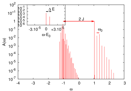
Figure 1: Electron spectral function for $\gamma=0.1$ $\lambda=2$and $T=0$ see ref. [8].

4.2 The static approximation

The case, in which a light quantum particle interacts with much more massive particles, is very common in solid state and molecular physics. We discuss the adiabatic regime, meaning that, in a characteristic time for the the light particle dynamics, the heavy degrees of freedom can be considered approximately quiet. Here, we describe the SA approach in its basic formulation for the dynamics.

The Hamiltonian (1) can be written in the coordinate-momentum representation

$$H=\frac{p^{2}}{2m}+\frac{m\omega_{0}^{2}}{2}x^{2}-\frac{\bar{g}}{\sqrt{2}}x\sigma_{z}-J\sigma_{x}-\omega_{0},$$ (29)

with $\bar{g}=g\sqrt{2m\omega_{0}}$. In the adiabatic limit ($\gamma\ll 1$), the phonon is much slower than the electron (heavy phonon and large electron tunnelling amplitude) and one can neglect the phonon kinetic term in (29). This is the well known Born-Oppenheimer approximation. In practice, it consists in studying the electronic problem with $x$ as a classical parameter.

Within this approximation, we put $\omega_{0}=\sqrt{k/m}\rightarrow 0$ ($m$ is the ion mass) and the Hamiltonian becomes

$$H_{ad}=\frac{k}{2}x^{2}-\frac{\bar{g}}{\sqrt{2}}x\sigma_{z}-J\sigma_{x}.$$ (30)

The eigenvalues can be expressed trough the classical displacement $x$

$$V_{\pm}(x)=\frac{k}{2}x^{2}\pm\Omega(x),$$ (31)

with $\Omega(x)=\sqrt{\frac{\bar{g}^{2}}{2}x^{2}+J^{2}}$. The lowest branch ($-$) of (31) defines an adiabatic potential which has a minimum at $x=0$ as far as $\lambda<1$ while for $\lambda>1$, it becomes double well potential with minima at $\pm x_{m}$, $x_{m}=\sqrt{\frac{\bar{g}^{2}}{2k^{2}}-\frac{2J^{2}}{\bar{g}^{2}}}$, in this case the electron is mostly localized on a given site. The quantum fluctuations are able to restore the symmetry in analogy to what happens for an infinite lattice [23]. It is worth noticing that, in this limit, Hamiltonian (1) is equivalent to the adiabatic version of the spin-boson Hamiltonian [24, 25].

The temporal evolution is given by

$$e^{-iH_{ad}t}=e^{-i\frac{kx^{2}}{2}t}[\cos\Omega(x)t+i(\frac{\bar{g}x}{\sqrt{2}\Omega(x)}\sigma_{z}+\frac{J}{\Omega(x)}\sigma_{x})\sin\Omega(x)t],$$ (32)

so the density matrix dynamics can be explicitly calculated

The electronic initial preparation, corresponds to the density matrix

$$\rho(0)=|1\rangle\langle 1|\sqrt{\frac{k\beta}{2\pi}}\int dx\,e^{-\frac{\beta k}{2}x^{2}}|x\rangle\langle x|,$$ (33)

tracing out the phonon we obtain the electron reduced density matrix with elements

$$\rho^{(el)}_{2,2} = \sqrt{\frac{\beta J\lambda}{2\pi}}\int du\,e^{-\frac{\beta J\lambda}{2}u^{2}}\frac{\sin^{2}(Jt\sqrt{u^{2}\lambda^{2}+1)}}{1+\lambda^{2}u^{2}}$$

$$\rho^{(el)}_{1,2} = -i\sqrt{\frac{\beta J\lambda}{2\pi}}\int du\,e^{-\frac{\beta J\lambda}{2}u^{2}}\frac{\sin(2Jt\sqrt{u^{2}\lambda^{2}+1})}{2\sqrt{\lambda^{2}u^{2}+1}}$$ (34)

where the scaled lenght $u=xk\sqrt{2}/\bar{g}$ was introduced.

In the same way, we can introduce the polaronic preparation

$$\rho(0)=|1\rangle\langle 1|e^{-\frac{\beta\bar{g}^{2}}{4k}}\sqrt{\frac{k\beta}{2\pi}}\int dxe^{-\beta(\frac{k}{2}x^{2}-\frac{\bar{g}}{\sqrt{2}}x)}|x\rangle\langle x|,$$ (35)

It is worth noting that, in the adiabatic limit, we cannot define the polaronic dynamics, as introduced in (7), because the operator $D$ is not defined for $\omega_{0}=0$. In this limit, we study electronic dynamics with an initial polaronic preparation. The corresponding reduced density matrix is

$$\rho^{(pol)}_{2,2} = \sqrt{\frac{\beta J\lambda}{2\pi}}\int_{-\infty}^{\infty}du\,e^{-\frac{\beta J\lambda}{2}(u-1)^{2}}\frac{\sin^{2}(Jt\sqrt{(u\lambda)^{2}+1})}{(u\lambda)^{2}+1}$$

$$\rho^{(pol)}_{1,2} = \sqrt{\frac{\beta J\lambda}{2\pi}}\int_{-\infty}^{\infty}du\,e^{-\frac{\beta J\lambda}{2}(u-1)^{2}}\left[\frac{u\lambda\sin^{2}(Jt\sqrt{(\lambda u)^{2}+1})}{((\lambda u)^{2}+1)}\right.$$ (36)

$$- \left.i\frac{\sin(2Jt\sqrt{(\lambda u)^{2}+1})}{2\sqrt{(\lambda u)^{2}+1}}\right]$$

It is possible to show that $\rho^{(pol)}_{2,2}$ is actually the adiabatic limit of the diagonal element of the reduced polaronic density matrix, while this is not true for the off-diagonal elements.

We want to stress that, in the SA approach, the phonon is completely static because its momentum $p$ has been neglected. Here, only the initial phonon distribution plays a role, but during electron hopping, oscillator is taken to be fixed.

4.3 A quantum-classical dynamics approximation

To account for dynamics of the slow variable, a mixed quantum-classical dynamics can be introduced. In the past, several schemes for quantum-classical dynamics has been proposed, for example starting from the Born-Oppenheimer (SA) adiabatic approximation for the ground state at each step and using a density functional Hamiltonian [26, 27]. Another approach, good for a short time dynamics, consists in a mapping from the Heisenberg equations to a classical evolution by an average over the initial condition[28, 29]. Some schemes are based on the evolution of the density matrix coupled to a classical bath [30, 31]. A systematic expansion over the mass ratio has also been done, starting from partial Wigner transform of the Liouville operator, in [32, 33, 34]. The QC approximation we use is essentially that of refs. [30, 31].

Let us consider Hamiltonian (29), where $x$ and $p$ are assumed to be classical variables which can be represented as the components of a vector $\mathbf{u}$. Then a QC state vector can be introduced as

$$\mathbf{v}=\mathbf{u}\otimes\mathbf{\sigma}=\left(\begin{array}[]{c}x\\ p\\ \sigma_{x}\\ \sigma_{y}\\ \sigma_{z}\end{array}\right).$$ (37)

The classical variables evolve with the Ehrenfest equations

$$\left\{\begin{array}[]{ccl}\dot{x}&=&\frac{p}{m}\\ \dot{p}&=&\frac{m\omega_{0}^{2}}{2}x-\frac{\bar{g}}{\sqrt{2}}\left\langle\sigma_{z}\right\rangle,\end{array}\right.$$ (38)

while the quantum variables evolves in the Heisenberg picture

$$\left\{\begin{array}[]{ccl}\dot{\sigma}_{x}&=&-\sqrt{2}\bar{g}x\sigma_{y}\\ \dot{\sigma}_{y}&=&\sqrt{2}\bar{g}x\sigma_{x}-2J\sigma_{z}\\ \dot{\sigma}_{z}&=&2J\sigma_{y}\end{array}\right..$$ (39)

To give a unified description of the overall evolution, we define a Liouvillian operator $\mathcal{L}=\mathcal{L}_{x}+\mathcal{L}_{p}+\mathcal{L}_{\sigma}$ with

$$\mathcal{L}_{\sigma}=-i\left(\begin{array}[]{ccc}0&-\sqrt{2}\bar{g}x&0\\ \sqrt{2}\bar{g}x&0&-2J\\ 0&2J&0\end{array}\right)$$ (40)

and $\mathcal{L}_{x}=\dot{x}\frac{\partial}{\partial x}$ $\mathcal{L}_{p}=\dot{p}\frac{\partial}{\partial p}$. So, the time evolution is given by

$$\mathbf{v}(t)=e^{i\mathcal{L}t}\mathbf{v}(0).$$ (41)

The numerical integration can be implemented using the symmetries Trotter breakup formula [35, 36]

$$\mathbf{v}(t)\simeq\left(e^{i\mathcal{L}_{\sigma}\frac{\epsilon}{2}}e^{i\mathcal{L}_{p}\frac{\epsilon}{2}}e^{i\mathcal{L}_{x}\epsilon}e^{i\mathcal{L}_{p}\frac{\epsilon}{2}}e^{i\mathcal{L}_{\sigma}\frac{\epsilon}{2}}\right)^{N}\mathbf{v}(0)$$ (42)

with $\epsilon=t/N$. All the density matrix elements, can be expressed in terms of elements of $\mathbf{v}(t)$.

5 Results

5.1 Antiadiabatic regime

In figure 2 is shown the time behaviour of the purity $P$ (Eq. (10)) as well as the transition probability ( (9)) obtained in the antiadiabatic regime when the phonon frequency ($\omega_{0}$) is much larger than electron hopping $J$ for both (el) (3) and (pol) (4) initial preparations. Timescales defined in section are shown as vertical lines, the time scale is logarithmic to better show the much different time domains. We consider two parameters sets at several temperatures. One characteristic of strong coupling (left panels) and the other of weak coupling (right panel). The same sets of parameters and temperatures is used in figure 3 where with show the time-averaged $P$ and $w$. Let us first discuss the strong coupling regime.

It is known that, in the antiadiabatic regime, the polaron is a well defined quasi-particle at strong coupling [37], in the sense that, in the polaronic spectral function, almost all the spectral weight is contained in the polaronic peak. This has also been shown for a two-site model [8, 14, 15, 38, 39, 40]. On the contrary, in the electron spectral function, the total spectral weight is distributed between a large number of frequencies [8].

From the point of view of transition probability and purity, the strong dependence on initial preparation can be seen comparing the low temperature evolution for both the actual (figure 2 left panel) and the time-averaged (figure 3 left panel) quantities.

Let us consider the electron preparation (Figs. 2 3 bottom left panels). Here the coupling with the oscillator mode is strong and the system starting from a disentangled state (equation (3)) evolves in a state in which electron is entangled with the oscillator. This is shown in the purity evolution where we see that electron loses coherence very rapidly, on a time scale $\tau_{J}$, and becomes a mixed ensemble, even at zero temperature.

On the same timescale, transition probability approaches $1/2$ in average (figure 3 bottom left panel). The initial decoherence is almost independent on the temperature, as can be seen from averaged quantities, while long time recoherence peaks are suppressed as $T$ increases. Such a suppression results from destructive interference between time evolution of the different terms appearing in (6) when excited oscillator states are initially populated. Referring to the spectral analysis [8] and to figure 1, this phenomenon must be ascribed to the superposition of a large number of high frequency excitations.

Even if the transfer does not have a regular shape, one can see some high frequency oscillations of period $\tau_{\omega_{0}}$. These frequencies correspond to the energy separation between two adjacent electronic bands [8].

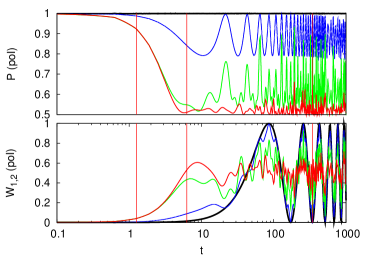
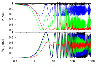
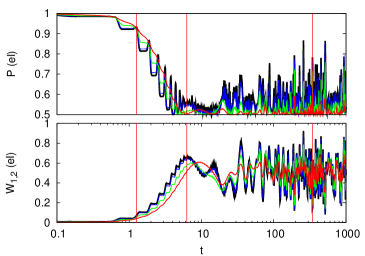
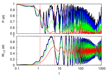
Figure 2: Polaron (top) and electron (bottom) populations and purity. Left panels antiadiabatic and strong coupling regime: $\gamma=10$ $\lambda=40$. Right panels antiadiabatic and weak coupling regime $\gamma=10$ $\lambda=10$. Curves are for $T/\omega_{0}=0.0$ (black), $T/\omega_{0}=0.5$ (blue), $T/\omega_{0}=2.0$ (green), $T/\omega_{0}=10.0$ (red). Vertical lines marks from left to right the timescales $\tau_{\omega_{0}}$,$\tau_{J}$,$\tau_{Q}$.

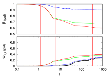
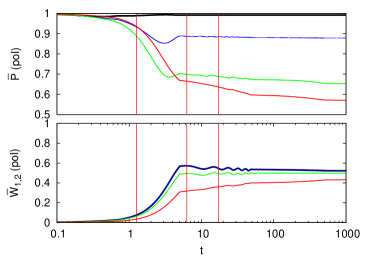
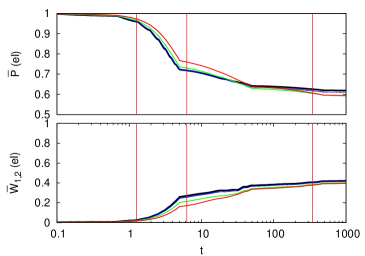
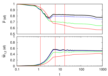
Figure 3: Polaron (top) and electron (bottom) time-averaged populations and purity. Parameters and labels are the same of figure 2.

On the contrary, the polaron preparation (see figure 2, top left panel) evolves in a state which is completely coherent at zero temperature. The frequency associated to polaron transfer is equal to the renormalized tunnelling $J^{*}$, as predicted by the HLFA (see 48). So, the state is pure and delocalized. The polaron state remains coherent even for temperatures comparable with $\omega_{0}$, but higher frequency modulation appears making the state oscillate from a pure to a mixed one. Nevertheless, it is possible to see an overall modulation of the transition probability with the same period $\tau_{Q}$ even at the largest temperature. This is in contrast with the HLFA at $T\neq 0$ (47) which predicts that the polaron band decreases with temperature and consequently $\tau_{Q}$ increases. However the purity decreases as temperature increases, as shown in figure 2. This is an effect of the broadening of the polaron band that is observed as temperature increases [8]. Indeed, a distribution of spectral weight among several poles around the polaron band occurs as an effect of increasing vibronic excitations (ref. [8] figure 3 upper panel). This leads to a decoherence effect due to destructive interference between these oscillating contributions to purity (see Eqs. (20,27)). For high temperature ($T\gg\omega_{0}$), the state becomes completely mixed and the evolution of the polaron is analogous to that of the electron. This is evident from the highest temperatures curves shown in figure 3, left panels upper and bottom left. We conclude that the main source of decoherence is temperature for polaron, while the electron decoheres even at zero temperature due to the coupling with the vibronic mode.

This is also found in the weak coupling regime (electron preparation Figs. 2,3 bottom right panels). Here electron coherence approaches a value which is larger in average than that at strong coupling (figure 3) and decreases as temperature increases. We see (Figs. 2,3 right panels) that the polaron purity differs qualitatively from the electron only near zero temperature, while averaged polaron and electron transition probabilities is essentially the same for all showed temperatures. Indeed, a sufficiently weak interaction is not able, at zero temperature, to excite many vibrational states, so the electron decoherence is essentially given by the small perturbation of the lowest oscillator’s states. On the other hand, the polaron is not formed (we are below the polaron crossover) and the charge does not acquire much coherence by moving with the oscillation cloud. Spectral analysis shows (ref. [8] figure 3 lower panel) that in weak coupling HLFA is qualitatively recovered, we have a polaron band narrowing as temperature is raised up in contrast with the strong coupling behaviour.

It is worth stressing that, in both weak and strong coupling regimes, at high temperature, the increasing number of oscillator states involved in the initial state produce decoherence on timescale $\tau_{J}$. Decoherence can be partial but nonetheless no environment is needed to explain the decoherence process. The only source of decoherence are the states populated by the initial thermal distribution

5.2 Adiabatic regime

Results form the Exact Diagonalization method is reported in figure 4, the averaged quantities are shown in 5 in the same way we did in the antiadiabatic case. Notice that now the shortest timescale is $\tau_{J}$.

Let us first discuss the strong coupling case. We see that, in contrast with antiadiabatic regime, there is a marked dependency on temperature of both electron and polaron properties. More specifically, polaron preparation no longer evolve coherently at low temperature.

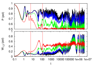
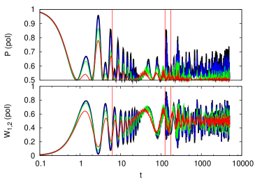
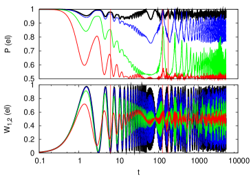
Figure 4: Polaron (top) and electron (bottom) populations and purity. Left panels Adiabatic and strong coupling regime: $\gamma=0.1$ $\lambda=2$. Right panels adiabatic and weak coupling regime $\gamma=0.1$ $\lambda=0.5$. Curves are for $T/\omega_{0}=0.0$ (black), $T/\omega_{0}=0.5$ (blue), $T/\omega_{0}=2.0$ (green), $T/\omega_{0}=10.0$ (red).Vertical lines marks from left to right the timescales $\tau_{J}$,$\tau_{\omega_{0}}$,$\tau_{Q}$.

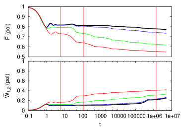
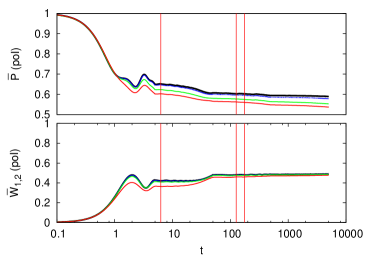
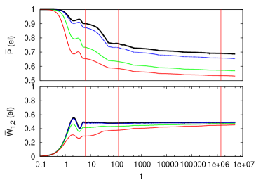
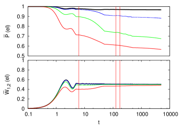
Figure 5: Polaron (top) and electron (bottom) time-averaged populations and purity. Parameters and labels are the same of figure 4

In the first time scale, $\tau_{J}$, the particle is localized (its transition probability is extremely low) but the state keeps on being quite pure. The polaron is trapped inside the initial site and both transition probability and coherence evolve initially with characteristic time $\tau_{J}$ independently on temperature. At intermediate timescale $\tau_{\omega_{0}}$ temperature induces delocalization while the coherence decreases. In this time regime, the polaron transition probability is related to the quasi classical motion of the oscillator and depends strongly on temperature.

This can be seen in figure 6, where we plot the temperature dependence of the level reached by the averaged transition probability on the time scale $\tau_{\omega_{0}}$ (inset). Since there is no clear plateau in the averaged transition probability for times greater than $\tau_{\omega_{0}}$, the choice of the transition probability level it is rather arbitrary. We choose the value of $\bar{w}_{12}$ at $\tau_{\omega_{0}}$. We see that this transition probability level pass from a low temperature behaviour, which is temperature independent, to a temperature dependent behaviour trough a wide crossover.

At very low temperature, after the characteristic time $\tau_{\omega_{0}}$, coherence and transition probability reach a quasi stationary value that is essentially dominated by fast tunnelling of the charge between the two sites, with a given phonon displacement. Once temperature increases, classical activation processes of the phonon coordinate becomes effective, producing an increase in transition probability as well as a decrease of the purity. As we shall see in the next section, this thermal activated behaviour is to be ascribed to the phonon classical hopping between two adiabatic minima and disappears in the SA where such hopping events are absent.

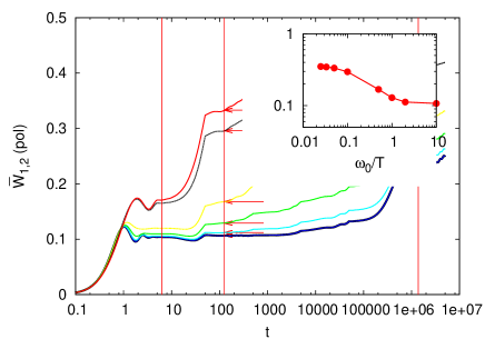
Figure 6: Time averaged transition probability for $\lambda=2.0$,$\gamma=0.1$, temperatures are from bottom to upper curves $T/{\omega_{0}}=0.1,0.5,1.0,2.0,10.0,20.0$. Vertical lines marks from left to right timescales $\tau_{J}$,$\tau_{\omega_{0}}$ and $\tau_{Q}$ respectively. Inset: levels reached at time $\tau_{\omega_{0}}$ (arrows in the main panel) as a function of the inverse temperature.

As far as electron is concerned, we can see that the site occupancy begins to oscillate coherently, with period $\tau_{J}$, with a damping increasing with temperature. In the same timescale, the time averaged value shows a saturation at low temperature. At a temperature independent intermediate timescale $\tau_{\omega_{0}}$, time averaged coherence reaches a very slowly decreasing level which decreases with increasing temperature. Quantum oscillations still exist further in time, but the remaining coherence slows down at high temperature, so that the long timescale ($\tau_{Q}$) seems to be not relevant in this case. The electron’s tendency to coherently hop is suppressed by decoherence, induced by excited phonons, whose number increases with temperature. In the adiabatic limit, this effect is more evident than in the antiadiabatic case, this is because the energy spacing between the oscillator’s levels becomes very small and the spectrum tends to a continuum.

In the weak coupling case (figure 4 and 5 right panels) the transition probability is very similar for both electron and polaron as in the antiadiabatic case. Conversely, at low temperature, the electron is much coherent than the polaron. In this regime, being the adiabatic potential single-well, the displaced phonon base is not the best choice. So, many displaced oscillator states are coupled with polaron, which decoheres rapidly.

5.3 Comparison with quanto-classical approaches

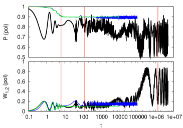
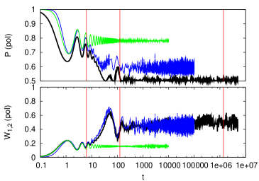
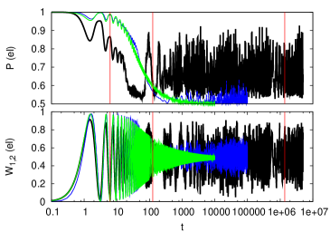
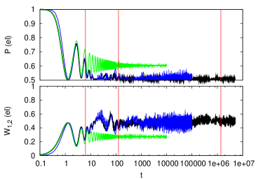
Figure 7: Polaron (top) and electron (bottom) populations and purity in the adiabatic strong coupling regime $\gamma=0.1$ $\lambda=2$. Left panels low temperature $T/\omega_{0}=0.1$. Right panels high temperatures $T/\omega_{0}=10.0$. Curves refers to ED (black), QC (blue), SA (green) approximations. Vertical lines marks from left to right the timescales $\tau_{J}$,$\tau_{\omega_{0}}$,$\tau_{Q}$.

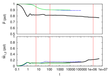
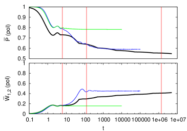
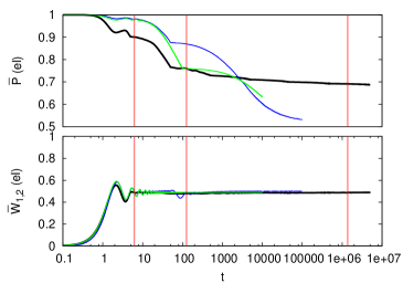
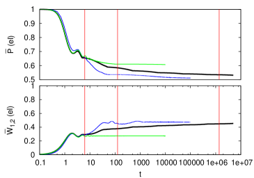
Figure 8: Polaron (top) and electron (bottom) time-averaged populations and purity. Parameters and labels are the same of figure 7

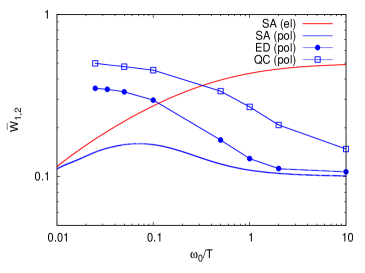
Figure 9: Time average transition probability level at the timescale $\tau_{\omega_{0}}$ in the adiabatic regime ($\lambda=2.0,\gamma=0.1$) as a function of inverse temperature for different preparations and different approximations.

In this section, we show a comparison between the results obtained in the three different ways described before: exact diagonalization (ED) by means of mapping introduced in Sec. 5.1, the quantum-classical (QC) dynamics approach described in Sect. 4.3 and the static (SA) approximation (Sect. 4.2). We shall limit ourselves to an adiabatic case ($\gamma=0.1$) with electron-phonon interaction strong enough to allow the polaron formation ($\lambda=2$).

In figure 7, is reported the exact dynamics given by the three different techniques, while in figure 8 is shown the time average. Remember that, as far as the polaron is concerned, in both SA and QC approximation, the purity represents that of the electron with a initially displaced phonon distribution.

At low temperature (left panels), and within the $\tau_{J}$ timescale, the classical phonon is almost freezed, and so both SA and QC approximation are equivalent. Nevertheless, the ED behaviour, of both polaron and electron preparation, is quite different because of quantum fluctuations. In particular, for short timescales, one can see that the ED dynamics, at low temperature, is damped faster than the other two approximations. The difference becomes more evident for higher timescales. In this regime, the temperature is not so effective in dissipation processes, while the strong coupling and the quantum uncertainty produce a sort of purely quantum damping.

A damping of this sort was also found in ref. [17], where authors consider a spin-boson Hamiltonian for a tunneling system coupled to a multi-mode bath with a ohmic spectral density. It is worth stressing that, in the present case, such a damping is not due to the bath but rather a consequence of the entanglement between the tunnelling system and the quantum oscillator. Nevertheless our results are comparable with that of ref. [17]. The reason is that, at strong coupling, the charge is coupled to the bath through a single collective mode, taking into account all the bath’s oscillators.

As expected, the exact polaron purity completely differs from the purity obtained by SA and QC. The reason is that, at low temperature and strong coupling, the polaron is well defined and moves as a quite coherent particle, as can be seen from the long timescale oscillations. On the contrary, if we consider only an electron with a displaced oscillator, the particle remains localized because the trapping mechanism, but it cannot coherently tunnel between the two sites.

A semiclassical behaviour is approached for $T$ greater than $\omega_{0}$, when SA and QC reproduce the ED transition probability within the $\tau_{J}$ timescale, as results evident in the right panels of Figs. (7-8). The QC approach remains a good description also for higher timescales. Notice that the same occurs in the transport of extended system where classical incoherent transport is achieved when $T$ is greater than $0.2\omega_{0}$ [41]. It is worth noticing that for very high temperature ($T\simeq J$,$T/\omega_{0}=10$ in figs. 8,9) the polaron is not formed, its dynamics approaches that of the electron in an initially delocalized phonon distribution. As a result, the QC purity approaches the ED’s.

At high temperature, the oscillator dynamics plays a relevant role, QC is a much better approximation of ED than SA. This fact can be understood by realizing that the main temperature effect is the damping of the coherent tunnelling oscillations. Once these oscillation are sufficiently suppressed, the phonon driven dynamics prevails. In the SA framework, the initial thermal distribution of the phonon coordinate makes the electron thermalizes irreversibly in a time that is the shorter the greater the temperature. Before this adiabatic thermalization, i.e, in a tunnelling period, the SA is still a good approximation.

Afterwards, the hopping of the oscillator coordinate into the other minimum of the adiabatic potential (equation (31)) takes place. The charge degree of freedom follows while $w_{1,2}$ saturates on average. In extended systems this regime corresponds activated mobility regime [42, 43, 44]. Since SA completely neglects the oscillator’s dynamics, it does not predict correctly $w_{1,2}$, as can be seen in figure 9. The QC approximation, instead, gives a correct qualitative prediction.

6 Conclusions

In this paper, we have studied a simplified model to treat the dynamics of a tunnelling charge interacting with a vibrational degree of freedom. We introduced a reduced density matrix approach to characterize the charge dynamics. Temperature is introduced by taking an initial equilibrium distribution of the oscillator. Both the transition probability and the purity are studied, in order to connect the charge transfer with its coherence.

Due to the simplicity of our model, we were able to span all the parameter’s space even at high temperature and strong coupling and to study the role of initial preparation. Moreover, we can explore a temporal range which is very large, compared with the typical time scales that can be obtained in models where the charge is coupled with a many degree of freedom oscillators’ bath [17, 45, 46].

As in any finite system, in our model, transition probability and purity can be expressed as a superposition of many non commensurate by oscillations. We therefore expect an oscillatory behaviour in our quantities of interests. However the initial thermal distribution of the oscillator states induces decoherence on intermediate timescale, due to the strong interaction with the oscillator. This phenomena occurs depending on initial preparation of the system.

We find that, in the antiadiabatic and strong coupling regime, the polaron exhibits a coherent tunnelling dynamics over time scales of the inverse polaron renormalized band. The coherent behaviour is lost out of the polaronic phase, i.e. increasing the temperature or decreasing the coupling. Electron evolves though partially incoherent dynamics. In the adiabatic strong coupling regime, temperature enhances the incoherent polaron charge transfer. The opposite occurs in the electron preparation.

In the adiabatic regime, two common approximations has been compared with exact results, the aim is to highlight the limits of validity of these approximations and to provide a simple testing tool, the two-site model, for generalizations to other extended models. As expected, a dynamical semi-classical approximation gives good estimates for both coherence and tunnelling amplitude, at high temperature $T\gg\omega_{0}$. Quite unexpectedly, it allows for a good approximation of the transition probability at low temperature, as far as time averaged quantities are concerned. However, such a quasiclassical approximation fails approaching the anti-adiabatic regime where non adiabatic transition are expected to contribute significantly to charge dynamics. This simplified model could serve to test approximate schemes to deal with this regime [45].

To conclude, we have shown that a non dissipative evolution of a tunneling system, strongly coupled to a single oscillator, can give rise to decoherence phenomena when the initial distribution of the oscillator is thermal and when the oscillator distribution is not initially equilibrated in the presence of the charge, that is sufficiently far from the thermal equilibrium distribution in the presence of the charge. These decoherence phenomena are independent on the presence of a dissipative bath. Thus, in a non equilibrium experiment in which a charge is introduced in a molecular system and interacts strongly with a particular mode of the molecular system, decoherence effects can be triggered alone by this coupling and by the initial non equilibrium distribution of the molecule.

Appendix

Atomic limit

In the atomic limit, the Hamiltonian is diagonalized by the so-called Lang-Firsov (LF) transformation

$$D=\rme^{\alpha\sigma_{z}(a^{\dagger}-a)}.$$ (43)

This transformation shifts the phonon operators by a quantity $\alpha$, while the electron operators are transformed in new fermionic operators, with energy $E_{p}$, associated to a quasi-particle called polaron[47, 12]. This particle can be tough as a charge moving together with a dressing cloud of oscillator quanta, $\alpha^{2}$ represents the mean number of phonons in the polaron cloud.

The atomic Hamiltonian

$$H_{0}=\omega_{0}a^{\dagger}a-\tilde{g}\sigma_{z}(a^{\dagger}+a),$$ (44)

after the LF transformation $\bar{H}_{0}=D^{\dagger}H_{0}D$ becomes:

$$\bar{H}_{0}=\omega_{0}a^{\dagger}a+E_{p}/2,$$ (45)

the eigenvalues $E_{n}=\omega_{0}n+E_{p}/2$ correspond to the two-fold degenerate eigenvectors $|\psi_{n}^{j},j\rangle=D|n,j\rangle=\bar{c}_{j}^{\dagger}|n\rangle$, were the index $n=0,\ldots,\infty$ refers to the photon number, $j=1,2$ to the electron site and $\bar{c}_{j}^{\dagger}$ is the polaron creation operator $\bar{c}_{j}^{\dagger}=Dc_{j}^{\dagger}D^{\dagger}=c_{j}^{\dagger}\exp\{(-1)^{j}\alpha(a^{\dagger}-a)\}$.

In the case of finite $J$, the hopping term is not diagonalized by (43) and the new Hamiltonian $\bar{H}=D^{\dagger}HD$ becomes

$$\bar{H} = \omega_{0}a^{\dagger}a-J(\sigma_{x}\cosh({2\alpha(a^{\dagger}-a)})+$$ (46)

$$+\rmi\sigma_{y}\sinh({2\alpha(a^{\dagger}-a)}))+E_{p}/2.$$

Depending on the choice of the parameters, the problem will be better described by a electron or polaron excitation picture. In particular, in the weak coupling limit, both the small polaron and the electron are good quasiparticle while, in the intermediate and strong coupling regimes, the polaron behaviour prevails [39].

The different regimes was widely studied, in literature, both for the two site problem and the extended case. The anti-adiabatic case was first studied in small $J$ perturbation regime [12, 48] and in the Holstein-Lang-Firsov approximation [12, 37] (HLFA), were an effective Hamiltonian is introduced to eliminate the phonon states. In HLFA $J$ is substituted by an effective hopping integral obtained by averaging the displacement $\exp{[2\alpha(a^{\dagger}-a)]}$ on the thermal distribution of phonons. The resulting effective hopping integral is

$$J^{*}=J\exp(-4\alpha^{2}(n_{B}(T)+1/2)),$$ (47)

where $n_{B}$ is the Bose occupation number. At zero temperature, the well known exponential reduction of the bandwidth is obtained

$$J^{*}=J\exp(-2\alpha^{2})$$ (48)

and, as the temperature is increased ($T/J>>\gamma$), the bandwidth decreases rapidly. As we shown in ([8]) and in the present paper, this is a good approximation at zero temperature but it becomes inadequate at finite $T$ where incoherent processes turns out to be important.

References

References

- [1] Jean J M 1994 J. Chem. Phys. 101 10464–10473
- [2] LeRoy B J, Lemay S G, Kong J and Dekker C 2005 Nature 432 371
- [3] Zazunov A, Feinberg D and Martin T 2006 Phys. Rev. B 73 115405 (pages 15)
- [4] Kovalenko S A, Dobryakov A L and Farztdinov V 2006 Physical Review Letters 96 068301
- [5] Kamada H, Gotoh H, Temmyo J, Takagahara T and Ando H 2001 Phys. Rev. Lett. 87 246401
- [6] Berciu M 2007 Phys. Rev. B 75 081101
- [7] Fulton R and Gouterman M 1961 J. Chem. Phys. 35 1059
- [8] Paganelli S and Ciuchi S 2006 J. Phys.:Condens. Matter 18 7669
- [9] Paganelli S and Ciuchi S 2007 ArXiv e-prints 710 (Preprint 0710.4096)
- [10] Swain S 1973 J. Phys. A 6 192
- [11] Cini M and D’Andrea A 1988 J. Phys. C 21 193
- [12] Holstein T 1959 Ann. Phys. 8 343
- [13] Firsov Y A and Kudinov E K 1997 Phys. Solid State 39 1930–1937
- [14] Ranninger J and Thibblin U 1992 Phys. Rev. B 45 7730–7738
- [15] de Mello E V L and Ranninger J 1997 Phys. Rev. B 55 14872–14885
- [16] Herfort U and Wagner M 1999 Philosophical Magazine B 79 1931
- [17] Lucke A, Mak C H, Egger R, Ankerhold J, Stockburger J and Grabert H 1997 J. Chem. Phys. 107 8397
- [18] Wagner M and Köngeter A 1989 Phys. Rev. B 39 4644
- [19] Wagner M 1984 J. Phys A 17 2319
- [20] Feinberg D, Ciuchi S and de Pasquale F 1990 Int. J. Mod. Phys. B 4 1317
- [21] Capone M and Ciuchi S 2002 Phys. Rev. B 65 104409
- [22] Herfort U and Wagner M 2001 J. Phys.:Condens. Matter 13 3297
- [23] Gerlach B and Löwen H 1987 Phys. Rev. B 35 4291
- [24] Weiss U 1993 Quantum Dissipative Systems (World Scientific)
- [25] Breuer H and Petruccione F 2003 The Theory of Open Quantum Systems (Oxford University Press, Oxford)
- [26] Car R and Parrinello M 1985 Phys. Rev. Lett. 55 2471–2474
- [27] Selloni A, Carnevali P, Car R and Parrinello M 1987 Phys. Rev. Lett. 59 823–826
- [28] Golosov A A and Reichman D R 2001 J. Chem. Phys. 114 1065–1074
- [29] Stock G 1995 J. Chem. Phys. 103 1561–1573
- [30] Berendsen H J C and Mavri J 1993 J. Phys. Chem 97 13464
- [31] Morozov V, Dubina Y and Shorygin P 2004 Int. J. Quant. Chem. 96 226
- [32] Kapral R and Ciccotti G 1999 J. Chem. Phys. 110 8919–8929
- [33] Nielsen S, Kapral R and Ciccotti G 2001 J. Chem. Phys. 115 5805–5815
- [34] Sergi A 2006 J. Chem. Phys. 124 4110 (Preprint quant-ph/0511142)
- [35] Wan C C and Schofield J 2000 The Journal of Chemical Physics 112 4447–4459 URL http://link.aip.org/link/?JCP/112/4447/1
- [36] De Raedt H and De Raedt B 1983 Phys. Rev. A 28 3575–3580
- [37] Lang I G and Firsov Y A 1963 Sov.Phys. JETP 16 1301
- [38] de Mello E V L and Ranninger J 1998 Phys. Rev. B 58 9098–9103
- [39] Robin J M 1997 Phys. Rev. B 56 13634
- [40] Alexandrov A S, Kabanov V V and Ray D K 1994 Phys. Rev. B 49 9915
- [41] Fratini S and Ciuchi S 2003 Phys. Rev. Lett. 91 256403
- [42] Kudinov E K and Firsov Y A 1965 Sov. Phys. Solid State 7 435
- [43] Kramers H A 1940 Physica 7 284
- [44] Hänggi P, Talkner P and Borkovec M 1990 Reviews of Modern Physics 62 251–342
- [45] Bonella S and Coker D F 2005 J. Chem. Phys. 122 4102–+
- [46] Egger R and Mak C H 1994 Phys. rev. B 50 15210
- [47] Tiablikov S V 1952 Zh. Eksp. Teor. Fiz. 23 381
- [48] Appel J 1967 Solid State Physics ed Ehrenreich H, Seiz F and Turnbull D (Academic Press) p 193