Strong horizontal photospheric magnetic field
in a surface dynamo simulation

Abstract

Context. Observations with the Hinode spectro-polarimeter have revealed strong horizontal internetwork magnetic fields in the quiet solar photosphere.

Aims. We aim at interpreting the observations by means of results from numerical simulations.

Methods. Radiative MHD simulations of dynamo action by near-surface convection are analyzed with respect to the relation between vertical and horizontal magnetic field components.

Results. The dynamo-generated fields show a clear dominance of the horizontal field in the height range where the spectral lines used for the observations are formed. The ratio between the averaged horizontal and vertical field components is consistent with the values derived from the observations. This behavior results from the intermittent nature of the dynamo field with polarity mixing on small scales in the surface layers.

Conclusions. Our results provide further evidence that local near-surface dynamo action contributes significantly to the solar internetwork fields.

1 Introduction

The ubiquitous existence of small-scale ‘internetwork’ magnetic fields of mixed polarity in the so-called quiet solar photosphere is strongly indicated by various observational diagnostics (e.g., Khomenko et al., 2003; Lites & Socas-Navarro, 2004; Trujillo Bueno et al., 2004, and further references therein). Recent high-resolution space-borne observations with the spectropolarimeter of the Solar Optical Telescope aboard the Hinode satellite have considerably strengthened the case for internetwork fields and, furthermore, have revealed that the measured internetwork flux is dominated by strongly inclined, almost horizontal magnetic field (Lites et al., 2007; Orozco Suárez et al., 2007b). Considerable amounts of highly time-dependent horizontal magnetic flux have also been found in ground-based observations with lower spatial resolution (Harvey et al., 2007). The ubiquity of the small-scale, mixed-polarity internetwork field suggests a local origin of at least a significant part of the measured flux. Recently, we have demonstrated by means of radiative magneto-convection simulations that local dynamo action by near-surface convective flows is a possible source for the internetwork flux (Vögler & Schüssler, 2007). Here we show that the spatial structure of the dynamo-generated field provides a natural explanation for the observed dominance of the horizontal field component in the middle photosphere.

2 Numerical model

We use the results of dynamo run C of Vögler & Schüssler (2007) with $648\times 648\times 140$ grid cells in a computational box with a physical size of $4.86\times 4.86$ Mm² in the horizontal and 1.4 Mm in the vertical direction, the latter ranging from about 900 km below to 500 km above the average level of continuum optical depth unity at 630 nm wavelength $(\tau_{630}=1)$. The simulation has been run with the MURaM code (Vögler, 2003; Vögler et al., 2005). With a magnetic Reynolds number of about 2600, the simulation shows an exponential growth of a weak seed field with an $e$-folding time of about 10 minutes. The magnetic energy saturates at about 2.5% of the kinetic energy of the convective flows, the maximum of the spectral energy distribution lying at horizontal spatial scales of a few hundred km, at which scales the field displays a distinctly mixed-polarity character.

3 Relation of horizontal and vertical field components

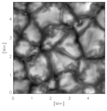
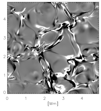
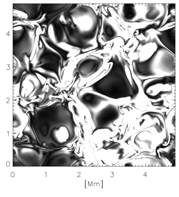
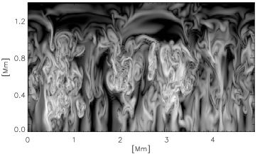
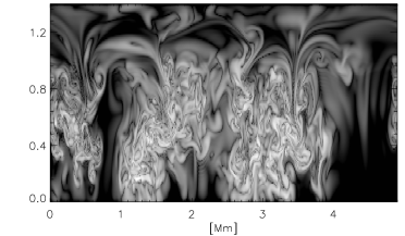
Figure 1: Snapshot from the saturated phase of the dynamo run C (Vögler & Schüssler, 2007). The panels in the upper row show the continuum intensity at 630 nm wavelength (upper left), a gray-scale image (‘magnetogram’, saturated at $\pm 10\,$G, black and white colour indicating the two polarities) of the (signed) vertical field component on the surface $\tau_{630}=10^{-2}$, roughly corresponding to the formation height of the spectral line used for the observations (upper middle), and the unsigned horizontal field strength (upper right), black colour in this panel representing very weak field and white colour indicating the saturation level of $10\,$G. The two panels in the lower row show gray-scale images of the logarithm of the horizontal field strength (black colour indicating fields below $1\,$G) for vertical cuts through the simulation box along a horizontal line at $y=1.5\,$Mm (left) and $y=3\,$Mm (right), respectively, in the upper panels. The level of $\tau_{630}=1$ is roughly at a height of $0.9\,$Mm, the level of $\tau_{630}=10^{-2}$ at $1.2\,$Mm.

Figure 1 is based upon a snapshot from the saturated phase of the dynamo run. The intensity image in the upper left panel shows the granulation pattern, which is almost undisturbed by the presence of the magnetic field. The distribution of the vertical field component on the level surface $\tau_{630}=10^{-2}$ (upper middle panel) reveals the mixed-polarity nature of the dynamo-generated magnetic field, which preferentially resides in the intergranular downflow lanes. Note that the distribution of vertical field at this level is significantly smoother than at the height of optical depth unity (cf. Fig. 2 of Vögler & Schüssler, 2007). This reflects the fact that much of the small-scale flux at the lower level has already been connected back by shallow loops. As a consequence, the unsigned vertical field drops much more rapidly with height than the (unsigned) horizontal field, so that at the level $\tau_{630}=10^{-2}$ the latter (shown in the upper right panel) dominates in most places. The representation on the two vertical cuts shown in the lower row of Fig. 1 illustrates that the horizontal field in the photosphere (i.e., above a height of about $0.9\,$Mm) has two components, namely, narrow loops near the intergranular lanes and extended loops above granules. The latter have also been seen in the simulations of Grossmann-Doerth et al. (1998) and Steiner (2007); they are presumably formed by reconnection events between loop ‘legs’ with opposite polarities and flux expulsion by the granular flows, larger (stronger) granules pushing the horizontal field to higher levels in the photosphere. As a consequence, a cut at a given level surface of constant height (or optical depth) as shown in the upper right panel of Fig. 1 misses part of the horizontal field above granules and will be more dominated by the field around the intergranular lanes. Lites et al. (2007) report that the observed horizontal field is spatially separated from the vertical field and favors the edges of bright granules. A comparison with this finding requires an analysis based upon synthetic Stokes profiles from the simulation data, which will be presented in a later paper.

Figure 2: Profiles of magnetic field strength averaged over surfaces of constant $\tau_{630}$: unsigned vertical field ($\langle|B_{z}|\rangle$, dashed), unsigned horizontal field components ($\langle|B_{x,y}|\rangle$, dotted and dash-dotted, respectively), and root-mean-square of the horizontal field strength ($\langle B_{x}^{2}+B_{y}^{2}\rangle^{1/2}$, solid).

A quantitative account of the relation between vertical and horizontal field components is given in Fig. 2. It shows field strengths averaged over surfaces of constant optical depth as functions of $\tau_{630}$. The dashed curve gives the average unsigned vertical field while the dotted and dash-dotted curves represent the averages of the two horizontal field components (unsigned).

The averages of the three components indicate that the field is not far from being statistically isotropic in the deep layers below $\tau_{630}=1$. In contrast, the horizontal components of the magnetic field become increasingly dominant in the photosphere above. The driving of the dynamo by small-scale turbulent shear flows in and adjacent to the intergranular downflows is mainly restricted to the regions below $\tau_{630}=1.$, whereas, in the convectively stable photosphere above, these flows are much weaker and the rate of work against the Lorentz force drops steeply with height. Since inductive effects have smaller influence on the field in the layers above $\tau_{630}=1$, the decay of the field with height is mainly determined by its spatial structure at the surface (particularly by the energy spectrum as a function of horizontal wavenumber). This results in a steep decline of the unsigned vertical field with height as opposite polarities on small scales are connected by shallow loops with typical length scales of a few hundred km, corresponding to the horizontal scale for which the magnetic energy spectrum at $\tau_{630}=1$ reaches its maximum. It becomes plausible that this configuration leads at the same time to a less steep decline of the horizontal field, if one considers the simple example of an arcade-like magnetic field with concentric semi-circular field lines: for increasing height, more and more field lines turn over horizontally, so that the horizontally averaged unsigned vertical field strength decreases faster than the averaged horizontal field; a simple calculation for this case shows that $\langle|B_{\rm hor}|\rangle$ strongly exceeds $\langle|B_{\rm vert}|\rangle$ at heights of the order of the horizontal scale (footpoint separation at the surface) of the arcade. Thus, the dominance of horizontal fields in the photosphere is consistent with the assumption of a simple loop topology with a preferred length scale.

The quantity that is actually relevant for a qualitative comparison with the ‘apparent’ horizontal field strength derived by Lites et al. (2007) from measurements of the linear polarization (transversal Zeeman effect, Stokes $Q$ and $U$) is the root-mean-square of the horizontal magnetic field, i.e., $B_{\rm rms}\equiv\langle B_{x}^{2}+B_{y}^{2}\rangle^{1/2}$, since for not too strong fields Stokes $Q$ and $U$ are proportional to the square of the horizontal field strength. $B_{\rm rms}$ as a function of optical depth is shown as the solid line in Fig. 2. Owing to the inhomogeneity of the horizontal field, this quantity is significantly larger than $\langle|B_{x}|\rangle$ and $\langle|B_{y}|\rangle$, even if we multiply any of them by a factor $\sqrt{2}$ to take into account both horizontal field components. From the ratio of the average horizontal field and the rms field, we can estimate an average ‘fill fraction’ as a measure of the inhomogeneity of the horizontal field. We obtain a number between 0.25 and 0.3 in the range $-2<\log\tau_{630}<-1$, which is the relevant range of line formation of the FeI lines at 630.15 nm and 630.25 nm used by the Hinode spectro-polarimeter (e.g., Orozco Suárez et al., 2007a). These values are consistent with the estimate of the fill fraction obtained by Lites et al. (2007) and Orozco Suárez et al. (2007b) by means of an inversion method.

Figure 3: Ratio of the root-mean-square of the horizontal field component (solid line in Fig. 2) to the averaged unsigned vertical field (dashed line in Fig. 2). In the optical depth interval $-2<\log(\tau_{630})<-1$ (relevant for the formation of the FeI lines used in the Hinode SP), the ratio is roughly in the range 4–6.

Let us now consider the ratio between the average vertical field and $B_{\rm rms}$ as shown in Fig. 3. The ratio increases strongly with height, so that in the optical depth interval $-2<\log\tau_{630}<-1$ values between 4 and 6 are reached. This is consistent with the ratio of the horizontally averaged vertical (longitudinal) and horizontal (transversal) apparent fields found by Lites et al. (2007): $B^{L}_{\rm app}/B^{T}_{\rm app}=55\,{\rm G}/11\,{\rm G}=5$. However, as pointed out by these authors, the relation between $B^{T}_{\rm app}$ and the actual horizontal field strength is far from trivial. Furthermore, effects of line-of-sight integration and spatial smearing by the instrument complicate the relationship between the average fields in the simulation and the field strengths derived from the observed Stokes profiles. A direct quantitative comparison with the observations would have to proceed by means of calculating synthetic Stokes profiles, taking into account the point-spread function of the instruments. This is beyond the scope of this Letter.

Lites et al. (2007) have suggested that one possibility contributing to the imbalance of the average vertical and horizontal fields could be a significantly larger horizontal scale of the horizontal field as compared to the vertical field. In fact, this is what we clearly find in our dynamo simulation. Fig. 4 shows spectral magnetic energy as a function of horizontal wave number. The dashed curve gives the energy distribution for the vertical field, while the solid curve represents the spectral energy in the horizontal field (mean of the spectra for the two horizontal field components). For this plot we have considered fields in the height range roughly corresponding to the optical depth interval $-2<\log\tau_{630}<-1$, which is relevant for the formation of the iron lines used for the observations. The curves show that the field components are in equipartition at small scales (large wave numbers), but that the horizontal field clearly dominates at wave numbers below roughly 10 Mm^-1, corresponding to horizontal scales larger than about 600 km.

Figure 4: Magnetic energy spectra as a function of horizontal wave number, $k$, for the height range roughly corresponding to $-2<\log\tau_{630}<-1$. The dashed curve shows the energy spectrum based on the vertical field component, while the solid curve gives the arithmetic mean of the spectra for the two horizontal field components. For low wavenumbers, the energy in the horizontal field clearly dominates.

4 Discussion

A direct comparison of the simulation results with the observations is not possible because the individual values for the averaged fields in the simulation are both (by about a factor three) smaller in the relevant height range than the values for the ‘apparent’ derived from the observation, the discrepancy probably becoming even more severe when the actual spatial resolution of the observations is taken into account. This is not particularly surprising since the magnetic Reynolds number of the simulation is still orders of magnitude smaller than the actual value in the corresponding solar layers, so that the saturation level of our simulation is probably considerably below the level to be expected for the real Sun. In fact, a preliminary simulation with a roughly doubled Reynolds number of about 5000 shows an increase of the magnetic energy by a factor of about 1.7 with respect to the case shown here. Interestingly, it turns out that the optical depth profiles of the averaged field strengths in this case can be very well approximated by just multiplying the curves shown in Fig. 2 by $\sqrt{1.7}$, meaning that the main difference between the simulations reduces to a simple scale factor for the field strength. Together with the fact that the observed internetwork fields are predominantly weak and their energy is significantly smaller than the kinetic energy of the convective motions, this suggests that the general nature of the dynamo-generated field may not be significantly different from the case shown here, apart from a higher overall amplitude. In particular, we expect that the ratio of the average horizontal and vertical field is not strongly affected by the amplitude of the dynamo-generated field. Of course, these assertions need to be demonstrated by further simulations with higher Reynolds numbers.

The clear dominance of the horizontal field in the mid photosphere seems to be a rather specific property of the strongly intermittent field generated by near-surface turbulent dynamo action. Accordingly, the dynamo simulation of Abbett (2007, with a closed bottom boundary and a local treatment of radiative transfer) also exhibits strong horizontal field in the photospheric layers. On the other hand, models with an imposed net vertical flux (e.g., Vögler et al., 2005) or our recent simulations of the decay of a granulation-scale mixed-polarity field (at magnetic Reynolds numbers below the threshold of dynamo action) do not show this behavior; in these cases, the intricate small-scale mixing of polarities that is characteristic for the dynamo does not dominate the field structure. The rapid decay with height of such a dynamo-generated field is also consistent with the apparent lack of strong horizontal field in the chromosphere (Harvey et al., 2007).

What are the alternatives to near-surface dynamo action? ‘Shredding’ of pre-existing magnetic flux (remnants of bipolar magnetic regions) cannot explain the large amount of observed horizontal flux since the turbulent cascade does not lead to an accumulation of energy (and generation of a spectral maximum) at small scales. On the other hand, such a behavior is typical for turbulent dynamo action. Flux emergence from the deeper convection zone in the form of granule-sized small bipoles would have to proceed such a high rate in order to maintain the ubiquitous strong horizontal fields that it probably would not have gone undetected in the past (see, however, Centeno et al., 2007). The sporadic appearance of horizontal internetwork fields (HIFs) described by Lites et al. (1996) and interpreted as small-scale flux emergence events seems to be unsufficient to explain the ubiquitous horizontal field now found with Hinode. On the other hand, flux recycling of an overall background flux by granulation probably represents a significant source of horizontal field in network and plage regions. Emergence of extended horizontal field strands in granules as observed by Ishikawa et al. (2007) is not seen in local dynamo simulations.

In the real Sun, probably all three sources, i.e., dynamo, shredded fields, and small-scale flux emergence from deeper layers, contribute to the internetwork flux in unknown amounts. In any case, the strong horizontal fields in the quiet photosphere inferred by the observations indicate that the source of these fields at the solar surface is a mixed-polarity field whose energy is mostly contained in those spatial scales where the dynamo-generated flux resides. Therefore, the observational results obtained with the Hinode SP together with the analysis presented here provides strong indication that surface dynamo action represents a significant source for the internetwork field in the solar photosphere.

References

- Abbett (2007) Abbett, W. P. 2007, ApJ, 665, 1469
- Centeno et al. (2007) Centeno, R., Socas-Navarro, H., Lites, B., et al. 2007, ApJ, 666, L137
- Grossmann-Doerth et al. (1998) Grossmann-Doerth, U., Schüssler, M., & Steiner, O. 1998, A&A, 337, 928
- Harvey et al. (2007) Harvey, J. W., Branston, D., Henney, C. J., & Keller, C. U. 2007, ApJ, 659, L177
- Ishikawa et al. (2007) Ishikawa, R., Tsuneta, S., Ichimoto, K., et al. 2007, A&A, submitted
- Khomenko et al. (2003) Khomenko, E. V., Collados, M., Solanki, S. K., Lagg, A., & Trujillo Bueno, J. 2003, A&A, 408, 1115
- Lites et al. (2007) Lites, B. W., Kubo, M., Socas Navarro, H., et al. 2007, ApJ, submitted
- Lites et al. (1996) Lites, B. W., Leka, K. D., Skumanich, A., Martinez Pillet, V., & Shimizu, T. 1996, ApJ, 460, 1019
- Lites & Socas-Navarro (2004) Lites, B. W. & Socas-Navarro, H. 2004, ApJ, 613, 600
- Orozco Suárez et al. (2007a) Orozco Suárez, D., Bellot Rubio, L. R., & del Toro Iniesta, J. C. 2007a, ApJ, 662, L31
- Orozco Suárez et al. (2007b) Orozco Suárez, D., Bellot Rubio, L. R., del Toro Iniesta, J. C., et al. 2007b, ApJ, 670, L61
- Steiner (2007) Steiner, O. 2007, in Modern solar facilities - advanced solar science, ed. F. Kneer, K. G. Puschmann, & A. D. Wittmann (Universitätsverlag Göttingen, Germany, http://webdoc.sub.gwdg.de/univerlag/2007/solar_science_book.pdf), 321
- Trujillo Bueno et al. (2004) Trujillo Bueno, J., Shchukina, N., & Asensio Ramos, A. 2004, Nature, 430, 326
- Vögler et al. (2005) Vögler, A., Shelyag, S., Schüssler, M., et al. 2005, A&A, 429, 335
- Vögler (2003) Vögler, A. 2003, PhD thesis, University of Göttingen, Germany, http://webdoc.sub.gwdg.de/diss/2004/voegler
- Vögler & Schüssler (2007) Vögler, A. & Schüssler, M. 2007, A&A, 465, L43