Measuring the deformation of a ferrogel sphere in a homogeneous magnetic field

Abstract

A sphere of a ferrogel is exposed to a homogeneous magnetic field. In accordance to theoretical predictions, it gets elongated along the field lines. The time-dependence of the elastic shear modulus causes the elongation to increase with time analogously to mechanic creep experiments, and the rapid excitation causes the sphere to vibrate. Both phenomena can be well described by a damped harmonic oscillator model. By comparing the elongation along the field with the contraction perpendicular to it, we can calculate Poisson’s ratio of the gel. The magnitude of the elongation is compared with the theoretical predictions for elastic spheres in homogeneous fields.

I Introduction

A sphere is the most perfect, most symmetric geometrical object. The Pythagoreans believed that the sun and the earth are perfect and thus spherical. Of course the rotation of the Earth is breaking the spherical symmetry. Whether this changes the shape of the Earth to a prolate or oblate rotational ellipsoid has been the subject of a long lasting quarrel between Newton and Cassini Chandrasekhar (1987). The breaking of the spherical symmetry is found to be important in various fields of physics. The efficiency of nuclear fission depends on the shape of the nucleus Bohr and Wheeler (1939). Particularly convenient is a breaking of the symmetry by an external electric or magnetic field. A drop of a magnetic liquid, a colloidal dispersion of magnetic nanoparticles Rosensweig (1985), elongates along the direction of the applied homogeneous magnetic field Bacri and Salin (1982, 1983); Flament et al. (1996). Very recently an amount of “quantum ferrofluid”, consisting of dipolar Cr-Atoms, has been found as well to elongate in a magnetic field Lahaye et al. (2007).

All examples presented above have in common that they deal with fluid bodies, without any elasticity. In contrast smart nanocomposite polymer gels Varga et al. (2003) are kept together by their elastic polymer matrix. Especially ferrogels Zrinyi et al. (1996); Zrínyi (2000) are a promising class for many applications, like soft actuators, magnetic valves, magnetoelastic mobile robots Zimmermann et al. (2006, 2007), artificial muscles Babincová et al. (2001), or magnetic controlled drug delivery Lao and Ramanujan (2004). All these applications are based on the magnetic deformation effect, a coupling between the mechanic and magnetic degrees of freedom.

The magnetic deformation effect is studied in its simplest form for a spherical gel body subjected to a homogeneous magnetic field. An approximation for the resulting deformation has been given in 1960 by Landau for the case of a dielectric elastic sphere Landau and Lifschitz (1960) and can readily be transferred to ferrogels Raikher and Stolbov (2003, 2005a); Raikher and Stolbov (2005b). The relative elongation $\varepsilon$ in this case was calculated as

$$\varepsilon=\frac{\kappa\mu_{0}}{G}M^{2}$$ (1)

where $\kappa=\nicefrac{{1}}{{15}}$, $G$ is the shear modulus and $M$ is the magnetization. Recently, the elongation has been recomputed by Raikher Raikher and Stolbov (2005a) without constraining the shape to an ellipsoid. In this case, the elongation is expected to be $30\,\%$ larger. This effect has not yet been observed, a possible reason being that it is rather small for the large values of $G$, characteristic for most of the covalently cross linked polymer gels  Zrinyi et al. (1996, 1997). In contrast, the elasticity of the new class of thermoreversible ferrogels  Lattermann and Krekhova (2006) can reversibly be tuned via their temperature. In the present paper, we cast thermoreversible ferrogels in spherical samples and expose them to a uniform magnetic field, to test the above predictions.

II Experiment

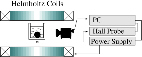
Figure 1: Scheme of the experimental setup.

II.1 Setup

Our experimental setup is sketched in Fig. 1. A ferrogel ball is immersed in a rectangular container, positioned on the common axis midway between two Helmholtz coils. For the empty Helmholtz pair of coils, the spatial homogeneity is better than $\pm 1\,\%$. This grade is valid within a cylinder of $1\,\mathrm{cm}$ in diameter and $14\,\mathrm{cm}$ in height oriented symmetrically around the center of the coils. The coils are powered by a current amplifier (fug electronic GmbH), which is controlled by a computer. The magnetic system cannot follow the control signal immediately. For a maximal jump height $\Delta B=36\,\mathrm{mT}$ the field is reached after $t_{B}=30\,\mathrm{ms}$, as recorded by the Hall probe (Group3-LPT-231) connected to a digital teslameter (DTM 141).

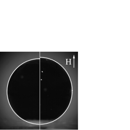
Figure 2: Image of the symmetrical (left) and distorted ball (right). The dotted line displays a fit with a circle (left) and an ellipse (right).

The temporal evolution of the ball shape is recorded using a highspeed camera, capable of taking $400$ frames per second with a resolution of $768\times 768$ pixels. Figure 2 shows the original and distorted shape. The dotted curves stem from a fit of a circle to the edges in the image. The circle is located utilizing a normalized correlation technique Dickey and Romero (1991), where the correlation between the gradient of the image and a circle is maximized. The gradient is estimated by the Sobel operator Wang et al. (uary), and the circle is rasterized with anti-aliasing provided by a Gaussian filter Crow (1977). This method is able to extract the radius and the coordinates of the center with subpixel resolution.

II.2 Material

The ball was prepared with a magnetic, thermoplastic elastomer gel or in other words with a thermoreversible ferrogel Lattermann and Krekhova (2006). Therefore, an ABA-type poly(styrene-b-(ethylene-co-butylene)-b-styrene) (SEBS) triblock copolymer (Kraton G-1650) was used as a gelator. As measured with size exclusion chromatography (SEC), Kraton G-1650 exhibits a molar mass of $99\,000$. The styrene content is $29\,\%$ (manufacturer information). The gelator concentration is $3.5\,\mathrm{w}\%$ per paraffin oil used. The ferrofluid was prepared in the classical way Lattermann and Krekhova (2006) with $24.5\,\mathrm{w}\%$ magnetite per paraffin oil Finavestan A 50 B (Total). The shear viscosity at $20\,$°C of $11\,\mathrm{mPa\,s}$ and the molar mass of $280$ (manufacturer information) are lower than that of the earlier used paraffin oil Finavestan A 80 B Lattermann and Krekhova (2006). Using A 80 B, the resulting ferrogels are too stiff to be remarkably deformed by the magnetic field. On the other hand, using the gelator Kraton G-1652 with a lower molar mass of $79\,000$ (SEC), the prepared ferrogels are still softer, i. e. they are even less shape-retaining. Furthermore, they sweat out ferrofluid, slowly on standing, faster in the magnetic field.

II.3 Sample preparation

Above its softening temperature at $45$°C the material becomes a magnetic liquid. We produce the ferrogel sphere by casting the liquid into an aluminum mould at $55$°C. The mould consists of two parts with a spherical cavity, tightly screwed together, which is connected by a thin channel to a hopper mounted on top of the upper part. To avoid any air bubbles in the final sphere, the mould is first filled with the liquefied material under vacuum ($\approx 1\,\mathrm{mPa}$). Then atmospheric pressure is applied, which compresses any low-pressure air bubbles. By repeating the process of varying the ambient pressure and under the influence of gravity, eventually all bubbles leave the mould via the hopper. Next we cool down the mould and separate the two parts of it.

The ball is then immersed into water with a temperature of 24°C, where all experiments have been carried out. The water contains an amount of salt, so that the density of the liquid is only slightly less than that of the ball. This is necessary to reduce the influence of the gravity on the shape of the sample; the ball is so soft that, without buoyancy, it is deformed into an oblate ellipsoid under gravity. As an additional benefit we can easily measure the density of the gel by examining the density of the fluid. The density determined by this method is $\rho=1.085\pm 0.005\,\mathrm{g/cm^{3}}$.

Figure 3: Magnetization curve of the ball.

II.4 Magnetization

Next, we measure the magnetization of the sphere for various fields, utilizing a fluxmetric magnetometer (Lakeshore, Model 480). The resulting magnetization curve is plotted in Fig. 3. The solid line displays an approximation with the model presented in Ref. Ivanov and Kuznetsova (2001). The sample is superparamagnetic with an initial susceptibility $\chi_{0}=0.81$.

Figure 4: The force response to a jump in the deformation. The solid line displays a fit to Eq. (2) with the parameters $G_{\text{rheo}}=1480\,\mathrm{Pa}$, $t_{0}=127\,\,\mathrm{s}$ and $\beta=0.218$.

II.5 Rheology

For the characterization of the elastic properties we measure the shear modulus $G$. with a rheometer (MCR 301, Anton Paar) in cone and plate geometry. The cone has a diameter of $50\,\mathrm{mm}$ and a base angle of $1$°. We perform a stress relaxation experiment on the sample: from the equilibrium position we shear the sample by a deformation of $\gamma=1\,\%$ and measure the stress $\tau$ as a function of time. Figure 4 displays the results. The restoring force decays by $50\,\%$ during one second, which means that the shear modulus $G=\tau/\gamma$ cannot be treated as constant. This decay can well be approximated by a stretched exponential (the solid line in Fig. 4)

$$G(t)=G_{\text{rheo}}\exp\left(-(\nicefrac{{t}}{{t_{0}}})^{\beta}\right).$$ (2)

The material therefore softens under load. To account for that time dependence, the magnetic experiment cannot be performed in a static manner.

Figure 5: Elastic response of the ball, when a magnetic field is suddenly applied. The solid line represents a fit to Eq. (3).

III Results and discussion

We performed time-resolved measurements of the relative elongation $\varepsilon$ of the ball after applying a magnetic induction $B$ in a jumplike fashion for ten different values of $B$. Figure 5 shows $\varepsilon(t)$ for the case $B=36\,\mathrm{mT}$. The elongation $\varepsilon=(d-d_{0})/d_{0}$ measures the scaled difference of the diameters in the direction of the field ($d$) and without a field ($d_{0}$). Due to the sudden increase of the magnetic field and the inertia of the ball, the latter performs uniaxial damped vibrations with a frequency $f=22.4\,\mathrm{Hz}$. When the oscillations cease, the elongation continues to grow due to the softening under load. Because the timescale of the softening is much larger than that of the oscillation, the experiment may be approximated by a harmonic oscillator pulled by a constant force, where the spring constant relaxes according to Eq. (2)

$$\ddot{\varepsilon}+\delta\dot{\varepsilon}+\omega_{0}^{2}\exp\left(-(\nicefrac{{t}}{{t_{0}}})^{\beta}\right)\,\varepsilon=F.$$ (3)

Here $\delta$ is the damping constant, $F$ the pulling force (i.e. related to the magnetic induction) and $\omega_{0}$ the natural frequency. A fit with that equation is displayed in Fig. 5 as the solid line. The ratio $F/\omega_{0}^{2}$ corresponds to the relative elongation in the equilibrium state if the spring constant would not change. Therefore, this ratio compares to the elongation predicted by the static theories.

Figure 6: a) The static elongation as a function of $M^{2}$. The circles (triangles) denote the elongation (contraction) parallel (perpendicular) to the applied field, respectively. The solid (dashed) line is the best linear fit. b) The frequencies of the initial vibrations obtained from Eq. (3).

The dependence of the elongation on the magnetization is shown in Fig. 6 a. For ten different values of the magnetic induction we have recorded and evaluated the elongation $\varepsilon$ of the ball. Figure 6 a presents the outcome for the elongation parallel ($\varepsilon_{z}$) and perpendicular ($\varepsilon_{x}$) to the magnetic field. The data have been plotted versus $M^{2}$. In agreement with Eq. (1) we find a linear relationship $\varepsilon_{i}=c_{i}M^{2}$ with $c_{z}=13.4\cdot 10^{-5}(\mathrm{\frac{m}{kA}})^{2}$ and $c_{x}=-6.1\cdot 10^{-5}(\mathrm{\frac{m}{kA}})^{2}$. Figure 6 b shows the oscillation frequency $f=\omega_{0}/(2\pi)$ versus $M^{2}$.

Next we compare the ratio of the slopes $c_{z}/c_{x}=\kappa_{z}/\kappa_{x}$ with the theoretical predictions. For a deformation restricted to an ellipsoidal shape and the assumption of a uniform strain field, the expressions given in Landau and Lifschitz (1960); Raikher and Stolbov (2005a) can be rewritten in terms of Poisson’s ratio $\sigma$

$$\kappa_{z}= \frac{3-2\sigma}{20\sigma+20}$$ (4a)

$$\kappa_{x}= \frac{1-4\sigma}{20\sigma+20}.$$ (4b)

For an incompressible gel ($\sigma=1/2$) this leads to $\kappa_{z}=\frac{1}{15}$. For arbitrary $\sigma$ one obtains for the ratio

$$\kappa_{x}/\kappa_{z}=\frac{1-4\sigma}{3-2\sigma}.$$ (5)

We exploit Eq. (5) to determine $\sigma$, and by substituting $\sigma$ in Eqs. (4b,1) one finally arrives at $G$. This yields

$$\sigma=0.48\pm 0.01\quad G=0.65\,\mathrm{kPa}.$$ (6)

For the more general case of a non-uniform strain field and a shape not restricted to an ellipsoid Raikher and Stolbov (2005a), one obtains

$$\kappa_{z}= -\frac{6\sigma^{2}+\sigma-7}{20\sigma^{2}+48\sigma+28}$$ (7a)

$$\kappa_{x}= -\frac{\sigma^{2}+2\sigma}{10\sigma^{2}+24\sigma+14}$$ (7b)

which yields

$$\kappa_{x}/\kappa_{z}=\frac{2\sigma^{2}+4\sigma}{6\sigma^{2}+\sigma-7}$$ (8)

and finally gives

$$\sigma=0.47\pm 0.01\quad G=0.87\,\mathrm{kPa}.$$ (9)

Figure 7: The shear modulus measured by different methods: Commercial rheometer (dashed), elongation theoryRaikher and Stolbov (2005a) (short dashed), elongation theoryLandau and Lifschitz (1960)(dash-dotted), vibrations (solid circles).

Both approaches yield a Poisson’s ratio $\sigma$ very close to the limit of incompressibility $\sigma=\nicefrac{{1}}{{2}}$, which is characteristic for rubberlike materials Rinde (1970). As reported before Raikher and Stolbov (2005a), the values derived for the shear modulus $G$ differ by $\approx 30\,\%$. But the value obtained from the rheometer, $G_{\text{rheo}}=1.48\,\mathrm{kPa}$, exceeds the old and new predictions by a factor of $2.3$ and $1.7$, respectively. So none of them is corroborated by the experiment.

The frequency of the vibrations after the sudden increase of the magnetic field offers another possibility to measure the shear modulus. For an incompressible elastic sphere that performs spheroidal vibrations, where the sphere gets alternately deformed into a prolate and oblate ellipsoid of revolution, the frequency is given Love (1944) by

$$f=0.848\sqrt{\frac{G}{4\rho r^{2}}}.$$ (10)

Since the radius of the sphere $r$ and the density $\rho$ are known, we can compute the shear modulus from the measured vibration frequency $f$. Figure 7 shows a comparison of the value of the shear modulus obtained from $f$ with the values from the elongation and the mechanical measurement. The average shear modulus determined by this method is $G_{\text{vib}}=0.1\,\mathrm{kPa}$, which differs by a factor of $15$ from $G_{\text{rheo}}$. This large deviation may arise, because the model for the vibrations does not take into account the surrounding water. This needs to oscillate together with the sphere, leading to an increased effective mass of the oscillator, and thus a reduced frequency.

Figure 8: The shear deformation as a function of time, after applying a constant deformation of $1.2\,\%$ for $800\,\mathrm{s}$.

Now we reconsider the deviation between the shear modulus $G$ as determined from the elongations and $G_{\text{rheo}}$ determined via rheology. They differ by factor of about two. This difference cannot be explained solely by the inaccuracy of the measurement of $G_{\text{rheo}}$, which is typically around $10\,\%$ for a commercial rheometer. Rather, the deviation is likely to stem from the fact that the idealistic models Landau and Lifschitz (1960); Raikher and Stolbov (2005a) consider only Hookean elasticity, which is insufficient for our material. In fact, the deformation of a gel put under load can be made up of three contributions, namely instantaneous elastic deformation, retarded anelastic deformation and viscous flow Strobl (1997). Our material clearly shows anelasticity, as demonstrated in Fig. 4. Moreover, our sample shows the phenomenon of viscous flow, as illustrated in Fig. 8. In this measurement we first apply a constant strain for $800\,\mathrm{s}$, and then record the relaxation of the strain for zero stress. The remaining deformation at $t=7000\,\mathrm{s}$ is about $15\,\%$ of the strain initially applied. This value can be regarded as an upper bound for the plastic contribution to the deformation (viscous flow). While the existence of anelasticity and viscous flow gives no straight-forward explanation of the $70\,\%$ deviation between experiment and theory, it is obvious that the full viscoelastic behaviour of the gel should be included in the computations from the very beginning.

IV Conclusion

We have measured the deformation of a ferrogel sphere in response to a uniform magnetic field by direct optical means. We compare the results for the first time with the models in Refs. Landau and Lifschitz (1960); Raikher and Stolbov (2005a). From the ratio of the elongation parallel and perpendicular to the field, we calculate Poisson’s ratio, which is close to the value $\sigma=0.5$ expected for an incompressible material. More importantly, the absolute value of the elongation is $70\,\%$ larger than the one calculated from the models. This is presumable caused by the neglection of the anelasticity and viscous flow of the ferrogel. So further theoretical investigation, including the full viscoelastic properties of the gel, is needed to explain the experiment quantitatively. With such a model one would also be able to compute the dynamic response of the gel under a sudden change of the external magnetic field. This is not only of fundamental interest, but also important for possible technical applications of these smart materials.

V Acknowledgments

The authors thank Helmut R. Brand and Yurij L. Raikher for fruitful discussions. Financial support by the Deutsche Forschungsgemeinschaft via FOR 608 is gratefully acknowledged. A.T. is grateful for an INTAS Young Scientists Fellowship (05-109-4521). We thank Total (Finavestan A 50 B) and Kraton Polymers (Kraton G-1650) for providing samples.

References

- Chandrasekhar (1987) S. Chandrasekhar, Ellipsoidal Figures of Equilibrium (Clarendon Press, New York, 1987).
- Bohr and Wheeler (1939) T. Bohr and J. A. Wheeler, Phys. Rev. 56, 426 (1939).
- Rosensweig (1985) R. E. Rosensweig, Ferrohydrodynamics (Cambridge University Press, Cambridge, New York, Melbourne, 1985).
- Bacri and Salin (1982) J. C. Bacri and D. Salin, J. Phys. Lett. 43, L (1982).
- Bacri and Salin (1983) J.-C. Bacri and D. Salin, J. Phys. Lett. 44, 415 (1983).
- Flament et al. (1996) C. Flament, S. Lacis, J. Bacri, A. Cebers, S. Neveu, and R. Perzynski, Physical Review E 53, 4801 (1996).
- Lahaye et al. (2007) T. Lahaye, T. Koch, B. Fröhlich, M. Fattori, J. Metz, A. Griesmaier, S. Giovanazzi, and T. Pfau, Nature (London) 448, 672 (2007).
- Varga et al. (2003) Z. Varga, J. Feher, G. Filipcsei, and M. Zrinyi, Macromol. Symp 200, 93 (2003).
- Zrinyi et al. (1996) M. Zrinyi, L. Barsi, and A. Buki, J. Chem. Phys. 104, 8750 (1996).
- Zrínyi (2000) M. Zrínyi, Colloid. Polym. Sci. 278, 103 (2000).
- Zimmermann et al. (2006) K. Zimmermann, V. A. Naletova, I. Zeidis, V. Böhm, and E. Kolev, J. Phys. Condens. Matter 18, 2973 (2006).
- Zimmermann et al. (2007) K. Zimmermann, V. A. Naletova, I. Zeidis, V. Böhm, V. A. Turkov, E. Kolev, M. V. Lukashevich, and G. V. Stepanov, J. Magn. Magn. Mater. 311, 450 (2007).
- Babincová et al. (2001) M. Babincová, D. Leszczynska, P. Sourivong, P. Čičmanec, and P. Babinec, Journal of Magnetism and Magnetic Materials 225, 109 (2001).
- Lao and Ramanujan (2004) L. Lao and R. Ramanujan, Journal of Materials Science: Materials in Medicine 15, 1061 (2004).
- Landau and Lifschitz (1960) L. D. Landau and E. M. Lifschitz, Electrodynamics of Continuous Media, vol. 8 (Pergamon, Oxford, 1960), 3rd ed.
- Raikher and Stolbov (2003) Y. L. Raikher and O. V. Stolbov, Journal of Magnetism and Magnetic Materials 258-259, 477 (2003).
- Raikher and Stolbov (2005a) Y. L. Raikher and O. V. Stolbov, Journal of Applied Mechanics and Technical Physics 46, 434 (2005a).
- Raikher and Stolbov (2005b) Y. L. Raikher and O. V. Stolbov, Journal of Magnetism and Magnetic Materials 289, 62 (2005b).
- Zrinyi et al. (1997) M. Zrinyi, L. Barsi, D. Szabo, and H.-G. Kilian, The Journal of Chemical Physics 106, 5685 (1997).
- Lattermann and Krekhova (2006) G. Lattermann and M. Krekhova, Macromol. Rapid Commun. 27, 1373 (2006).
- Dickey and Romero (1991) F. M. Dickey and L. A. Romero, Opt. Lett. 16, 1186 (1991), URL http://www.opticsinfobase.org/abstract.cfm?URI=ol-16-15-1186.
- Wang et al. (uary) S. Wang, F. Ge, and T. Liu, EURASIP J. Appl. Signal Process. 2006, 213 (uary), ISSN 1110-8657.
- Crow (1977) F. C. Crow, Commun. ACM 20, 799 (1977), ISSN 0001-0782.
- Ivanov and Kuznetsova (2001) A. O. Ivanov and O. B. Kuznetsova, Phys. Rev. E 64, 041405 (2001).
- Rinde (1970) J. Rinde, Journal of Applied Polymer Science 14, 1913 (1970).
- Love (1944) A. Love, A Treatise on the Mathematical Theory of Elasticity (Courier Dover Publications, 1944).
- Strobl (1997) G. Strobl, The Physics of Polymers: Concepts for Understanding Their Structures and Behavior (Springer, 1997).