Investigating Heating and Cooling in the BCS & B55 Cluster Samples

Abstract

We study clusters in the BCS cluster sample which are observed by Chandra and are more distant than redshift, $z>0.1$. We select from this subsample the clusters which have both a short central cooling time and a central temperature drop, and also those with a central radio source. Six of the clusters have clear bubbles near the centre. We calculate the heating by these bubbles and express it as the ratio $r_{\rm heat}/r_{\rm cool}=1.34\pm 0.20$. This result is used to calculate the average size of bubbles expected in all clusters with central radio sources. In three cases the predicted bubble sizes approximately match the observed radio lobe dimensions.

We combine this cluster sample with the B55 sample studied in earlier work to increase the total sample size and redshift range. This extended sample contains 71 clusters in the redshift range $0\leq z\leq 0.4$. The average distance out to which the bubbles offset the X-ray cooling in the combined sample is at least $r_{\rm heat}/r_{\rm cool}=0.92\pm 0.11$. The distribution of central cooling times for the combined sample shows no clusters with clear bubbles and $t_{\rm cool}>1.2{\rm\thinspace Gyr}$. An investigation of the evolution of cluster parameters within the redshift range of the combined samples does not show any clear variation with redshift.

1 Introduction

Since the discovery of “holes” in the X-ray emission at the centre of the Perseus Cluster (Böhringer et al., 1993), and especially since the launch of Chandra and XMM-NEWTON, many depressions in the central intra-cluster medium (ICM) of low redshift clusters have been found (e.g. Hydra A, McNamara et al., 2000; A2052, Blanton et al., 2001; A2199, Johnstone et al., 2002; Centaurus, Sanders & Fabian, 2002). Recent compilations are given by Dunn & Fabian (2006); Rafferty et al. (2006) and Bîrzan et al. (2004). These holes have been observed to anti-correlate spectacularly with the radio emission from the active galactic nucleus (AGN) at the centres of these clusters. Their morphology, particularly in the closest clusters, has led to their interpretation as bubbles of relativistic gas blown by the AGN into the thermal ICM. The relativistic gas is less dense than the ICM, so the bubbles detach from the core and rise up buoyantly through the cluster, e.g. Perseus (Churazov et al., 2000; Fabian et al., 2003). The older bubbles tend not to have ${\rm\thinspace GHz}$ radio emission associated with them and have been termed “Ghost” bubbles.

The X-ray emission of the ICM represents an energy loss, so leads the plasma cooling in the core if there were no compensating energy source. To maintain pressure support, the gas would flow on to the central galaxy as a “cooling flow.” However, with the high spatial and spectral resolution of Chandra and XMM-Newton, the gas temperature is seen to drop by a factor of several in the core but no continuous cooling flow is found (Peterson et al., 2003, see Peterson & Fabian, 2006 for a review). Some form of gentle, continuous and distributed heating appears to be at work (Voigt & Fabian, 2004). The interaction of the AGN with the ICM is the likeliest explanation as the heat source for cool-core clusters. The bubble model for radio sources was proposed by Gull & Northover (1973), and further theoretical results were presented in Churazov et al. (2000, 2002). Recent studies on the heating ability of AGN within clusters are Bîrzan et al. (2004); Rafferty et al. (2006) and Dunn & Fabian (2006).

A majority (71 per cent) of “cooling core” clusters harbour radio sources (Burns, 1990), and a similar number of clusters which require heating (likely to be a cooling core) harbour clear bubbles (Dunn et al., 2005; Dunn & Fabian, 2006). The action of creating the bubbles at the centre of the cluster by the AGN is a favoured method of injecting energy into the central regions of the cluster and so prevent the ICM from cooling. This process sets up sound/pressure waves in the ICM, the dissipation of which requires the ICM is to be viscous (Fabian et al., 2003). The viscous dissipation of the pressure waves allows the energy from the bubble creation to be dissipated far from the cluster centre where it is required.

In Dunn & Fabian (2006) we analysed clusters in the Brightest 55 (B55) sample (Edge et al., 1990). These are all at comparatively low redshift (only two are at $z>0.1$). Using the results of Peres et al. (1998) and the literature at the time we selected those clusters with both a short central cooling time and a large central temperature drop, as well as those with a central radio source. We found that at least 70 per cent of clusters in which high cooling rates are expected (those with short central cooling times and central temperature drops) harbour AGN bubbles. We also found that 95 per cent of these cool core clusters harbour radio cores. The total fraction of clusters which harbour a radio source is 53 per cent (29/55). Where AGN bubbles are present, on average they show that the AGN is injecting enough energy into the central regions of the cluster to offset the X-ray cooling out to the cooling radius ($r_{\rm cool}$ where $t_{\rm cool}=3{\rm\thinspace Gyr}$). To increase the number of clusters studied and also investigate any evolution in the AGN heating with redshift we now turn to the Brightest Cluster Sample (Ebeling et al., 1998), initially performing a similar analysis and then combining the results from both cluster samples.

The sample selection for this work is outlined in Section 2 and the data preparation and reduction in Section 3. We then look at the two different cluster subsets, those with bubbles in Section 4 and those with central radio sources in Section 5. The results of our investigations into the global differences within the different subsets is presented in Section 6. The combined cluster sample and the redshift evolution results are presented in Section 7. We use $H_{0}=70\hbox{$\rm\thinspace km~{}s^{-1}~{}Mpc^{-1}$}$ with $\Omega_{\rm m}=0.3$, $\Omega_{\Lambda}=0.7$ throughout this work.

2 Sample Selection

Table 1: Cluster Sample

Cluster	Redshift	ObsId	Exposure (ks)	$t_{\rm cool}$	$T$ drop	Both	Bubbles	Radio
A68	0.255	3250	9.9
A115 N	0.197	3233	49.7	Y	Y	Y	Y	Y
A115 S	0.197	3233	49.7		Y
A267	0.227	1448	7.4
A520	0.202	528	9.5		Y
A586	0.171	530	10.0					Y
A665	0.182	531	8.9
A697	0.282	4217	19.5
A773	0.217	5006	19.8
A781	0.298	534	9.9		Y			Y
A963	0.206	903	35.9		Y
A1068	0.139	1652	25.5	Y	Y	Y		Y
A1201	0.169	4216	24.0
A1204	0.171	2205	23.3	Y
A1413	0.143	5003	75.0
A1423	0.213	538	9.7	Y	Y	Y		Y
A1682	0.226	3244	5.4		Y			Y
A1758 N	0.279	2213	49.7					Y
A1763	0.223	3591	19.5					Y
A1835	0.252	495	19.3	Y	Y	Y	Y	Y
A1914	0.171	3593	18.8
A2111	0.229	544	10.2		Y
A2204	0.152	499	10.1	Y	Y	Y		Y
A2218	0.171	1666	40.1
A2219	0.228	896	42.3					Y
A2259	0.164	3245	10.0
A2261	0.224	5007	24.3	Y
A2294	0.178	3246	9.0		Y
A2390	0.231	4193	89.8	Y	Y	Y		Y
A2409	0.147	3247	10.2
HercA	0.155	6257	49.4	Y	Y	Y	Y	Y
MS0906+1110	0.175	924	29.6
MS1455+2232	0.258	4192	91.4	Y	Y	Y		Y
RXJ0439+0520	0.208	1649	9.6	Y	Y	Y		Y
RXJ0439+0715	0.245	3583	19.2					Y
RXJ1532+3021	0.362	1649	9.2	Y	Y	Y	Y	Y
RXJ1720+2638	0.161	4361	23.3	Y	Y	Y		Y
RXJ2129+0005	0.234	552	9.9	Y	Y	Y		Y
ZwCl1953	0.373	1659	20.7					Y
ZwCl2701	0.214	3195	26.7	Y	Y	Y	Y	Y
ZwCl3146	0.285	909	45.6	Y	Y	Y	Y	Y
ZwCl5247	0.229	539	9.0					Y
Totals			42	16	21	14	6	23

All the clusters in the sample, for the sample selection see text. The exposure time is that after reprocessing the data. The cooling times and central temperature drops have been determined from the profiles calculated during the course of this work. Clusters with $<3{\rm\thinspace Gyr}$ are classed as having a short central cooling time, and those with $T_{\rm centre}/T_{\rm outer}<1/2$, a central temperature drop. The radio detections come from the NVSS.

To increase the number of clusters studied and to investigate the redshift evolution of AGN in clusters we now turn to the ROSAT Brightest Cluster Sample (BCS, Ebeling et al., 1998). Most of the B55 clusters are at low redshifts ($z\lesssim 0.1$), whereas the BCS clusters extend to higher redshifts. The BCS is a 90 per cent flux-complete sample comprising the 201 X-ray-brightest clusters in the northern hemisphere at high galactic latitudes ($|\,b\,|>20^{\circ}$ Ebeling et al., 1998). The member clusters have measured redshifts of $z\lesssim 0.4$ and fluxes greater than $4.4\times 10^{-12}{\rm\thinspace erg~{}cm^{-2}~{}s^{-1}}$ in the $0.1-2.4{\rm\thinspace keV}$ band (for $H_{0}=50\hbox{$\rm\thinspace km~{}s^{-1}~{}Mpc^{-1}$}$). There is a low flux extension to the BCS, the eBCS, which includes clusters with fluxes in the range $2.8\times 10^{-12}$ to $4.4\times 10^{-12}{\rm\thinspace erg~{}cm^{-2}~{}s^{-1}}$ (Ebeling et al., 2000). Bauer et al. (2005) investigated the existence of cool cores in the high redshift end of the BCS ($z>0.15$), and found that 34 per cent of clusters exhibited signs of strong cooling (central $t_{\rm cool}<2{\rm\thinspace Gyr}$). In our study ($z>0.1$ and $t_{\rm cool}<3{\rm\thinspace Gyr}$) we find that 16 clusters have a short central cooling time, corresponding to 38 per cent. If the temperature drop is also required for “strong cooling” then the fraction drops to 33 per cent, both of which match their result. Globally there have been a variety of estimates on the fraction of clusters which have cool cores Peres et al. (1998) used the B55 sample and found a fraction of 70-90 per cent. However they define a “cooling flow” cluster is that which has $t_{\rm cool}<t_{\rm cluster}=13{\rm\thinspace Gyr}$. If we use $t_{\rm cool}<13{\rm\thinspace Gyr}$ for our selection of cool core clusters, 38/42 (90 per cent) of clusters have a cool core. It is therefore reasonable to assume that the Chandra observations of clusters within the BCS have not been highly biased towards cool core clusters. In the B55 sample from Dunn & Fabian (2006) only 1/30 clusters would not have a cool core, though the selection procedure was different in that study.

So that the BCS and B55 cluster samples do not overlap in this study, we only select those clusters in the BCS with $z>0.1$ as the parent sample for this study. There is only one cluster in common with both the B55 and BCS with this cutoff, A2204. There are 87 clusters (including A2204) in the parent sample, of which 42 have observations in the Chandra archive. These are shown in Table 1. We assume that the Chandra observations have not been biased to a particular type of cluster and so quote population fractions from this sample of 42 rather than from the parent sample of 87 clusters.

Following the data reduction (see Section 3) this parent sample was further split into sub-samples, following Dunn & Fabian (2006): those clusters which harbour clear bubbles; those in which heating is required to prevent rapid cooling and those which harbour a radio source were identified. The allocation of clusters into the three sub-samples is shown in Table 1.

To identify those clusters which are likely to require some form of heating to prevent large quantities of gas from dropping out we take those which have a short central cooling time ($<3{\rm\thinspace Gyr}$) and a large central temperature drop ($T_{\rm centre}/T_{\rm outer}<1/2$). Exactly half (21) of the clusters in the sample have a central temperature drop, and 16 have a short central cooling time (16/42, 38 per cent, similar to Bauer et al. 2005, although they use $t_{\rm cool}<2{\rm\thinspace Gyr}$). 14 clusters have both (14/42, 33 per cent), of which at least 6 have clear bubbles (6/14, 43 per cent; 6/42, 14 per cent). We use the NVSS to determine whether the clusters have a central radio source. 23 clusters harbour a central radio source (23/42, 55 per cent), including all those which require some form of heating. There appears to be a category of clusters which have cool cores and a radio source but in which no clear bubbles have been detected. Both in the B55 sample (Table 2 Dunn & Fabian (2006), $2^{\rm nd}$ column) and the BCS have these sorts of clusters, with similar fractions in each (5/30 in the B55 and 8/42 in the BCS).

Comparing with the B55 sample, Dunn & Fabian (2006) found that the fraction of clusters which require heating is 25 per cent, and which harbour a radio source is at least 53 per cent. Of the clusters which require some form of heating, at least 70 percent harbour clear bubbles and 95 percent harbour a central radio source.

In comparing the number of identified bubbles in the BCS and B55 sample it is expected that as a result of the greater distance of clusters in the BCS, fewer bubbles would be identified even if the same proportion of clusters harboured them. It is therefore not surprising that the percentage of clusters which harbour bubbles is half that determined for the B55 (from those clusters which require heating). The proportion of clusters which harbour radio sources, on the other hand, is very similar (BCS=55, B55=53 per cent) as is the proportion of clusters requiring heating (BCS=33, B55=25 per cent).

Figure 1: The distribution of $t_{\rm cool}$ in the BCS sample. The black bars indicate those clusters which harbour clear bubbles, and the grey ones, those with a central radio source. ZwCl5247, which harbours a radio source, is beyond the right edge of this plot.

3 Data Preparation

The X-ray Chandra data of the clusters were processed and cleaned using the CIAO software and calibration files (CIAO v3.3, CALDB v3.2). We began the reprocessing by removing the afterglow detection and re-identifying the hot pixels and cosmic ray afterglows, followed by the tool acis_process_events to remove the pixel randomisation and to flag potential background events for data observed in Very Faint (VF) mode. The Charge-Transfer Efficiency was corrected for, followed by standard grade selection. Point-sources were identified using the wavdetect wavelet-transform procedure. For clusters observed with the ACIS-S3 chip, the ACIS-S1 chip was used to form the light curves where possible. In all other cases, light-curves were taken from on-chip regions as free as possible from cluster emission. For the spectral analysis, backgrounds were taken from the CALDB blank-field data-sets. They had the same reprocessing applied, and were reprojected to the correct orientation.

Cluster centroids were chosen to lie on the X-ray surface brightness peak. Annular regions, centred on the centroids, were automatically assigned with constant signal-to-noise, stopping where the background-subtracted surface brightness of the cluster dropped below zero. The initial signal-to-noise was 100, and this was increased or decreased by successive factors of $\sqrt{2}$ to obtain a number of regions between four and ten. The minimum signal-to-noise allowed was 10. For clusters imaged on the ACIS-I chip, the effects of excluding the chip-gaps was accounted for by adjusting the stop angles of the annuli.

The $0.5-7{\rm\thinspace keV}$ spectra were extracted, binned with a minimum of 20 counts per bin, and, using xspec (v12.3) (e.g. Arnaud 1996), a projct single temperature mekal (e.g. Mewe et al. 1995) model with a phabs absorption was used to deproject the cluster. Chi-square was used as an estimator of the spectral fit. In some clusters the temperatures for some of the regions were undefined. To solve this problem, the minimum number of regions was reduced, a maximum radius for the outermost annulus was set, or the outermost region was removed to try to improve the behaviour of the profile. Using the deprojected cluster temperature, abundance and normalisation profiles; density, pressure, entropy, cooling time and heating profiles were calculated.

These profiles give azimuthally averaged values for the cluster properties and have been used in the subsequent calculations. In some clusters, for example M87 and Perseus, the central parts of the cluster are not very smooth, e.g. due to bubbles. Donahue et al. (2006) show that these features do not strongly bias estimates of the entropy. As such the use of these azimuthally averaged values is not likely to introduce large biases into the subsequent calculations.

4 Clusters with Bubbles

The analysis of the clusters with clear bubbles is the same as in Dunn & Fabian (2006). Where clear cavities are seen in the X-ray emission then the energy injected into the central regions of the cluster is calculated from the energy in the bubbles.

$$E_{\rm bubble}=\frac{1}{\gamma_{1}-1}p_{\rm th}V+p_{\rm th}V=\frac{\gamma_{1}}{\gamma_{1}-1}p_{\rm th}V$$ (1)

where $V$ is the volume of the bubble, $p_{\rm th}$ is the thermal pressure of the ICM at the radius of the bubble from the cluster centre and $\gamma_{1}$ is the mean adiabatic index of the fluid in the bubble. Assuming the fluid is relativistic, then $\gamma_{1}=4/3$, and so $E_{\rm bubble}=4p_{\rm th}V$.

We parametrise the bubbles as ellipsoids, with a semi-major axis along the jet direction, $R_{\rm l}$, and a semi-major axis across it, $R_{\rm w}$. The depth of the bubbles along the line of sight is unknown and so we assume them to be prolate ellipsoids, with the resulting volume being $V=4\pi R_{\rm w}^{2}R_{\rm l}/3$.

To estimate the rate at which the AGN is injecting energy into the cluster the we need to estimate the age of the bubble. There are two principle methods of estimating the age of the bubble, the sound speed timescale and the buoyancy rise time. Observations of nearby clusters have shown that young bubbles which are still being inflated do not create strong shocks during their inflation. They are therefore assumed to be expanding at around the sound speed, and their age is $t_{\rm age}=t{c_{\rm s}}=R_{\rm l}/c_{\rm s}$ where the sound speed in the ICM is

$$c_{\rm s}=\sqrt{\gamma_{2}k_{\rm B}T/\mu m_{\rm H}}$$ (2)

where $\gamma_{2}=5/3$. As bubbles evolve they are expected to detach from the AGN and rise up buoyantly through the ICM (Churazov et al., 2000). Their age is best calculated by the buoyancy rise time; $t_{\rm age}=t_{\rm buoy}=R_{\rm dist}/v_{\rm buoy}$, with the buoyancy velocity given by

$$v_{\rm buoy}=\sqrt{2gV/SC_{\rm D}}$$ (3)

where $C_{\rm D}=0.75$ is the drag coefficient (Churazov et al., 2001) and $S=\pi R_{\rm w}^{2}$ is the cross-sectional area of the bubble.

The radio sources in this cluster sample are analysed after the identification of cavities within the X-ray emission. We find two strong radio sources within this sample, A115 (3C 28) and Hercules A (3C 348). Both have current radio emission in a bi-lobed morphology, and the radio lobes are still close to the core. None of the others have radio emission correlated with the cavities in the X-ray emission. We therefore assume that the radio emission has aged and so faded beyond the sensitivity limit, and class these bubbles as Ghost bubbles.

Using the deprojected temperature, density and abundance profiles, X-ray cooling was calculated for each spherical shell. This was compared to the power injected into the cluster by the AGN in the form of bubbles ($P_{\rm bubble}=E_{\rm bubble}/t_{\rm age}$). The distance out to which the bubble power can counteract the X-ray cooling was therefore calculated. Uncertainties have been estimated using a simple Monte Carlo simulation of the calculation.

Table 2: Clusters with Bubbles: Bubble Properties

Cluster	Bubble	Type	$R_{\rm l}$	$R_{\rm w}$	$R_{\rm dist}$
			( kpc)	( kpc)	( kpc)
A115	NE	Y	$32.1\pm 3.2$	$28.78\pm 2.8$	$39.0\pm 3.9$
	SW		$27.2\pm 2.7$	$20.3\pm 2.0$	$45.2\pm 4.5$
A1835	NE	G	$15.5\pm 1.6$	$11.6\pm 1.2$	$23.3\pm 2.3$
	SW		$13.6\pm 1.4$	$9.6\pm 1.0$	$16.6\pm 1.7$
HercA	E	Y	$110\pm 11$	$75.4\pm 7.5$	$110\pm 11$
	W		$124\pm 12$	$75.4\pm 7.5$	$124\pm 12$
RXJ1532+30	W	G	$23.5\pm 2.4$	$23.5\pm 2.4$	$32.0\pm 3.2$
ZwCl2701	E	G	$29.8\pm 3.0$	$29.8\pm 3.0$	$42.6\pm 4.3$
	W		$28.7\pm 2.9$	$28.7\pm 2.9$	$39.5\pm 4.0$
ZwCl3146	NE	G	$28.0\pm 2.8$	$28.0\pm 2.8$	$57.1\pm 5.7$
	SW		$30.0\pm 3.0$	$30.0\pm 3.0$	$53.2\pm 5.3$

The bubbles are parametrised as ellipsoids, with $R_{\rm l}$ the semi-major axis along the jet direction, and $R_{\rm w}$ the semi-major axis across it. We class young bubbles as those with clear radio emission, and ghost bubbles as those without. Both A115 (3C 28) and Hercules A (3C 348) have strong bi-lobed radio sources at their centres.

As this cluster sample is at a higher average redshift than the Brightest 55 sample studied in Dunn & Fabian (2006), fewer clear bubbles have been identified. Also, the X-ray emission is fainter, and so analysis of the outermost regions of the cluster becomes more difficult. Only large or extreme bubbles will be detected. It is therefore not surprising that of the six clusters which have clear depressions in the X-ray emission, in three of them the AGN is injecting much more energy than is being lost through X-ray emission in the central regions. Nulsen et al. (2005) have studied the Chandra data of Hercules A and concluded that this outburst is exceptionally powerful. A comparison between the X-ray cooling luminosity within the cooling radius to the bubble power is shown in Table 3.

Table 3: Clusters with Bubbles: AGN Heating ability

Cluster	$L_{\rm cool}^{\hskip 9.95863pta}$		$4p_{\rm th}V/t_{\rm age}$		$r_{\rm cool}$		$r_{\rm heat}$	$r_{\rm heat}/r_{\rm cool}^{\hskip 9.95863ptb}$		Heated Fractionc
	$(10^{43}{\rm\thinspace erg~{}s^{-1}})$		$(10^{43}{\rm\thinspace erg~{}s^{-1}})$		( kpc)		( kpc)
A115 N	$16.8$$\;\pm\;$	$1.1$	$273$$\;\pm\;$	$33$	$70.5$$\;\pm\;$	$3.8$	$>153$	$2.17$$\;\pm\;$	$0.12$	$16.4$$\;\pm\;$	$2.2$
A1835	$205$$\;\pm\;$	$6$	$190$$\;\pm\;$	$38$	$96.7$$\;\pm\;$	$2.3$	$90.5\pm 14.9$	$0.94$$\;\pm\;$	$0.16$	$0.92$$\;\pm\;$	$0.19$
HercA	$4.2$$\;\pm\;$	$0.4$	$1560$$\;\pm\;$	$360$	$45.9$$\;\pm\;$	$3.4$	$>600$	$13.1$$\;\pm\;$	$1.0$	$373$$\;\pm\;$	$98$
RXJ1532+30	$218$$\;\pm\;$	$23$	$331$$\;\pm\;$	$126$	$107$$\;\pm\;$	$10$	$187\pm 96$	$1.75$$\;\pm\;$	$0.91$	$1.52$$\;\pm\;$	$0.60$
ZwCl2701	$23.4$$\;\pm\;$	$1.9$	$602$$\;\pm\;$	$82$	$67.4$$\;\pm\;$	$3.0$	$>301$	$4.47$$\;\pm\;$	$0.20$	$25.5$$\;\pm\;$	$4.1$
ZwCl3146	$153$$\;\pm\;$	$7$	$786$$\;\pm\;$	$144$	$93.0$$\;\pm\;$	$3.7$	$>500$	$5.38$$\;\pm\;$	$0.21$	$5.11$$\;\pm\;$	$0.97$

The clusters in bold only have a lower limit for $r_{\rm heat}/r_{\rm cool}$ as the AGN counteracts all the cooling from the X-ray emission which could be analysed. ^a $L_{\rm cool}$ is calculated for the $0.5-7.0{\rm\thinspace keV}$ range. ^b The radius $r_{\rm heat}$, as a fraction of the cooling radius $r_{\rm cool}$, out to which the energy injection rate of the bubbles ($4p_{\rm th}V/t_{\rm age}$) can offset the X-ray cooling within that radius. ^c The fraction of the X-ray cooling that occurs within $r_{\rm heat}$.

The average distance, as a fraction of the cooling radius, out to which the bubbles can offset the X-ray cooling calculated from the results is presented in Table 3. The uncertainty in the mean was estimated using a simple bootstrapping method. On average, the clear bubbles in this sample counteract the X-ray cooling out to $r_{\rm heat}/r_{\rm cool}=1.34\pm 0.40$. The fraction of the X-ray cooling within the cooling radius offset by the action of the AGN is $1.22\pm 0.15$. We emphasise that this average is only for two clusters (A1835 and RXJ1532+30), and should be regarded as a lower limit for the following reasons.

The values exclude those clusters where the calculation only provides a lower limit on the distance. Adding these clusters into the calculation results in $r_{\rm heat}/r_{\rm cool}=4.31\pm 1.10$ and a heated fraction of $75.0\pm 50.4$. It is likely that, because of the greater average distance of this cluster sample, that the clusters with clear bubbles are those which are undergoing/have recently undergone powerful AGN outbursts. The more gentle energy injection events would not be easily identified in the X-ray emission.

We do not comment further on these results here, as there are only six clusters in this sub-sample. Further analysis, where these clusters are combined with those from the B55 sample, is discussed in Section 7.

5 Clusters with Radio Sources

All the clusters which require some form of heating harbour a radio source, which is similar to the fraction found by Dunn & Fabian (2006) of 95 per cent. Following the study in Dunn & Fabian (2006) we invert the problem, and use the results from the clusters with bubbles on this sample. Using the average distance out to which the bubbles counteract the X-ray cooling, we calculate the X-ray cooling luminosity for these clusters and equate this to the energy injected by the AGN.

$$P_{\rm bubble}=L_{\rm cool}(r<r_{\rm heat}),$$

where $r_{\rm heat}$ is calculated from $r_{\rm heat}=1.34r_{\rm cool}$. We assume that these “expected” bubbles are young, and so are being inflated at the sound speed.

$$R_{\rm bubble}=\sqrt{\frac{P_{\rm bubble}}{4p_{\rm th}c_{\rm s}}}$$

Uncertainties have been estimated using a simple Monte Carlo simulation of the calculation.

Table 4: Predicted Bubble Sizes

Cluster	$z$	$r_{\rm cool}$	Predicted Bubble Radius		Central	Radio dimensions
		$({\rm\thinspace kpc})$	$({\rm\thinspace kpc})$	(arcsec)	X-ray S/N	(arcsec)
A586	0.171	$20.59\pm 10.63$	$2.39\pm 1.00$	$0.82\pm 0.34$	1.7	-
A781	0.298	$20.96\pm 8.23$	$9.75\pm 2.04$	$2.18\pm 0.46$	1.3	$5.2\times 5.2$
A1068a	0.139	$77.19\pm 1.86$	$14.51\pm 2.23$	$5.91\pm 0.91$	59.6	$5.5\times 5.5$
A1423	0.213	$46.02\pm 8.68$	$5.89\pm 1.69$	$1.69\pm 0.49$	3.1	$3.9\times 10.3$
A1682	0.226	$27.82\pm 8.79$	$5.87\pm 1.07$	$1.61\pm 0.29$	1.1	$5.8\times 5.8$
A1758 N	0.279	$12.37\pm 12.17$	$4.82\pm 1.68$	$1.13\pm 0.40$	2.6	-
A1763	0.223	$18.38\pm 4.24$	$4.39\pm 0.55$	$1.22\pm 0.15$	2.0	$1.4\times 3.4$
A2204	0.152	$69.47\pm 3.19$	$9.08\pm 3.57$	$3.42\pm 1.34$	38.0	$5.0\times 5.0$
A2219	0.228	$20.55\pm 2.34$	$4.64\pm 0.29$	$1.26\pm 0.08$	5.3	$4.6\times 4.6$
A2390	0.231	$60.91\pm 1.16$	$10.81\pm 2.64$	$2.92\pm 0.71$	30.8	-
MS1455+2232	0.258	$96.56\pm 1.10$	$19.62\pm 4.26$	$4.88\pm 1.06$	65.4	-
RXJ0439+0520	0.208	$74.66\pm 6.20$	$11.81\pm 3.41$	$3.45\pm 1.00$	13.8	-
RXJ0439+0715	0.245	$40.18\pm 3.51$	$5.45\pm 0.29$	$1.41\pm 0.08$	3.3	-
RXJ1720+2638	0.161	$79.42\pm 2.77$	$12.64\pm 1.36$	$4.54\pm 0.49$	32.1	amorphous source
RXJ2129+0005	0.234	$72.78\pm 5.00$	$9.25\pm 2.86$	$2.47\pm 0.76$	8.5	-
ZwCl1953	0.373	$22.06\pm 8.33$	$4.48\pm 0.94$	$0.86\pm 0.18$	1.7	$3.7\times 3.7$
ZwCl5247b	0.229	$<78.54$	$<8.83$	$<2.4$	0.6	-

^a The radio emission from A1068 is discussed in more detail in the text. ^b The observation of ZwCl5247 is short for such a distant cluster. It also does not have a cooling core, although it appears to have a central radio source, and so the X-ray emission is not strongly peaked at the centre. The deprojection analysis results in a cooling time which is not well constrained at the centre. We therefore give only the upper limits for the values obtained by the analysis for the quantities in this table.

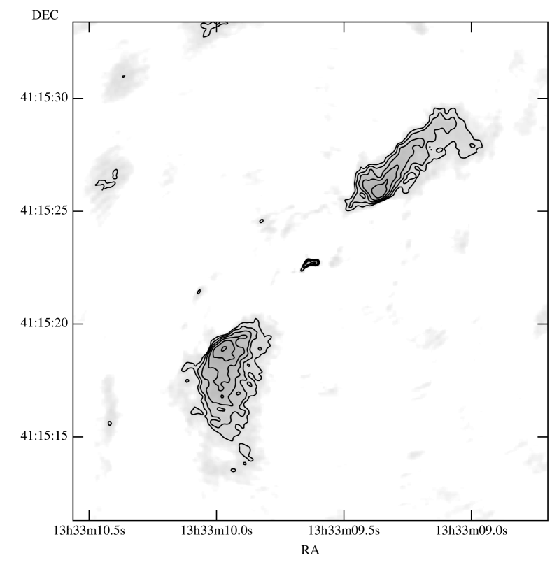
Figure 2: The $8{\rm\thinspace GHz}$ image of A1763 from the VLA in A-array. This is the only cluster in which bubbles are expected but none seen in the X-ray emission, which also has a bi-lobed radio source at the centre where the structure of the radio emission was resolved in the archival VLA data.

Using the size of an expected bubble in these clusters, the X-ray count total within the bubble was calculated from the current X-ray observation. This allowed the signal-to-noise of the observation to be obtained. The difference in counts between the bubble centre and the rims surrounding it was estimated from the bubbles in A2052 and Hydra A. The counts in the bubbles from these two clusters are around 30 per cent lower than the counts in the rims. If bubbles are present, then they would need to be detected above the noise at more than the $3\sigma$ level. For this to be the case, the signal-to-noise has to be greater than 13 (equivalent to noise at a 8 per cent level). However, as the cluster emission is changing over the scale of the bubbles the we may need a higher signal-to-noise to be able to detect any depressions. For a $5\sigma$ detection, the signal-to-noise required is 36. This does require knowing where the bubbles are so that the counts within the region where a bubble is expected can be compared to that outside. The results of this analysis are shown in Table 4.

There are six clusters (A1068, A2204, A2390, MS1455+2232, RXJ01439+0520 and RXJ1720+2638) where the central signal-to-noise of the observation is such that if there are bubbles present within this region, then with the aid of any radio emission to guide the eye, the bubbles should be detectable at the $3\sigma$ level. There are only three if the detection threshhold is lifted to $5\sigma$ (A1068, A2204 & MS1455), of which A1068 is discussed below, A2204 is discussed in Dunn & Fabian (2006) and no high resolution radio data was found for MS1455. As this signal-to-noise calculation has been calculated for the entire central part of the cluster, the value obtained may over estimate the signal-to-noise present at the location of the bubble if the core of the cluster is very bright.

The bi-lobed radio emission A1068 appears offset to the X-ray cluster centroid. It would be expected that for a typical double source, the lobes would sit either side of the X-ray peak (under the assumption that the AGN is in the very centre of the cluster). However, one “lobe” coincides with the peak in the ICM emission, the other occuring at $38{\rm\thinspace kpc}$ from the centre. In the vicinity of this more distant lobe, the signal to noise is $\sim 41$. As no clear features are seen in the X-ray emission, and the lobe locations are not typical, we investigated what this radio source is coincident with. Using the Sloan Digital Sky Survey (SDSS, Adelman-McCarthy & for the SDSS Collaboration 2007) we extracted images of the sky centred on the brightest cluster galaxy (BCG). Aligning the radio and optical images showed that the more distant (south-western) lobe is coincident with another galaxy in the cluster ($z=0.136$ compared to $z=0.138$ for the BCG). The central “lobe” is therefore an unresolved radio core. This would also explain the lack of bubble features in the high signal-to-noise X-ray emission, as no bubbles are seen, given the lack of extended radio emission.

Using the Very Large Array (VLA) archive we attempted to find observations of the clusters in which bubbles are expected to investigate the morphology of the central radio source. We analysed data at a variety of frequencies and array configurations, depending what was available in the archive and which had the longest time-on-source.

These clusters are all at redshifts higher than those in the B55 sample, and so we expected to resolve fewer of the central radio sources. Table 4 shows the expected bubble sizes and measured radio source dimensions. If no radio source dimensions are given then the source was not resolved in the observations that were analysed.

The predicted bubble and observed radio source sizes are very similar in A1068, A1763 (Fig. 2) and A2204. A1068 is discussed earlier in this section and A2204 was discussed in Dunn & Fabian (2006) and will not be covered further here. However, the radio source size and the X-ray observation signal-to-noise in A1763 are such that detecting any X-ray features of the bubble would be impossible, even with a much longer exposure. Under the assumption that the natural course of events when an AGN ejects radio emitting jets into the central regions of a cluster is that bubbles are formed, then, as in the B55 cluster sample Dunn & Fabian (2006), we are missing a large number of bubbles. This may be a timescale effect, currently in some of these clusters the AGN is not inflating bubbles, or they are present but too small to be detected with either the current X-ray or radio data.

In nearby clusters where X-ray and radio spatial resolution do not pose a problem for studying the morphology of the AGN and cluster, whenever there is a lobed radio source, there are always signs of an interaction between the relativistic and thermal plasmas. Therefore, for more distant objects, where even the spatial resolution of Chandra is insufficient to allow the detailed investigation of the interaction, perhaps the radio emission alone will be enough to determine the action of the AGN on the cluster. If the two plasmas do not significantly mix over a timescale of $\sim 10^{8}{\rm\thinspace yr}$, then if the AGN is actively producing jets, bubbles would be the natural consequence, along with the associated heating of the ICM. Therefore, if the bubbles do allow a good calibration of the AGN energy injection rate, the dimensions of the radio emission rather than of any X-ray features could be used to calculate the heating from the AGN.

6 Clusters requiring heating

All the clusters which require heating (but do not have clear bubbles – either reported or determined from the Chandra data) harbour a central radio source (as determined from the NVSS). Their expected bubble sizes have been calculated in Section 5.

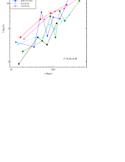
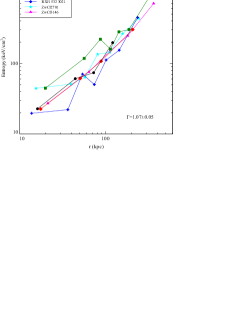
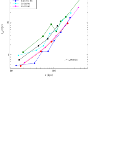
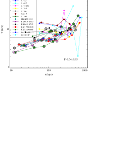
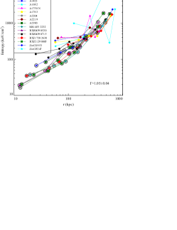
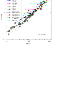
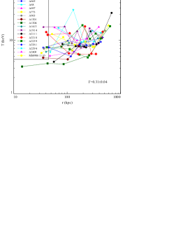
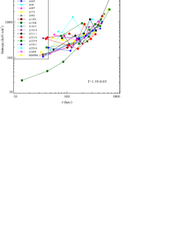
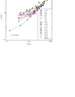
Figure 3: left: Temperature, centre: Entropy and right: Cooling time profiles for top: Clusters with clear bubbles, middle: Clusters with central radio sources and bottom: clusters with no central radio source. Best fitting powerlaw slopes, $(\Gamma)$, to all the date on the plots are shown. The clusters which require heating are highlighted by a large circle in the plots for the clusters harbouring a central radio source.

As a comparison between the three different sub-samples, Fig. 3 shows the temperature, entropy and cooling time profiles for the different sub-samples. There are only six clusters in the sub-sample containing clear bubbles and so small number statistics are relevant. Fig. 3 also shows the best fitting powerlaw slope to all the data points. It is interesting to note that in the average slope for all three parameters, the slope for the clusters with radio emission is always in between those with bubbles and those with neither. The temperature slopes of the radio and no-radio clusters are almost identical, whereas with the entropy and cooling time, it is the bubbled and radio clusters which have very similar slopes.

The clusters which require some form of heating are highlighted in Fig. 3. The clusters which require some form of heating do appear to be the coolest clusters and those which have the lowest central entropy. They are naturally those with the shortest central cooling time as this was one of the selection criteria. As is clear from Fig. 3, these clusters are those in which the deprojection resulted in the smallest central bin. As discussed in Bauer et al. (2005), the radius of the innermost annulus depends on the cluster distance and the signal-to-noise of the observation. The latter parameter is related to whether the cluster exhibits a cool core or not, as cool core clusters have higher central densities and hence have brighter X-ray cores.

There is a further possible bias towards having detailed/deep observations of cool core clusters and less deep observations of other clusters. A quick calculation of the average exposure for clusters which have bubbles, a radio source or neither results in $33.5$, $28.4$ and $24.3{\rm\thinspace ks}$ respectively. Although these exposure times are not significantly different (standard deviation $\geq 17$) it is interesting to note that the clusters which are of most interest to the heating and cooling balance are those which appear to have the longest exposure times. These clusters, as they are cool core, are also the brightest. For a balanced analysis the non-cool core clusters probably should have a longer average exposure times as they are less bright.

If the entropy data are split into those clusters which require some form of heating and those that do not, then there is a large difference in the slopes of the average entropy profiles. The different best fitting slopes are 1.01 and 0.72 respectively. Ignoring A1204 in the entropy fits for the clusters with no radio data results in a slope of 0.77. A1204 only just fails on the temperature drop selection criterion for requiring heating.

The average cooling time profiles of the clusters with bubbles and those with a radio source match the profiles presented in Voigt & Fabian (2004) of $t_{\rm cool}\propto r^{1.3}$.

7 Discussion

7.1 Combining the Samples

In order to study a large number of clusters over a range of redshifts we combine the BCS and the B55 samples. As A2204 is present in both we have used the central cooling time from the analysis presented in this manuscript in the following discussion. We therefore have $30+42-1=71$ clusters in the combined sample.

The B55 and BCS samples have slightly different selection criteria. The BCS sample selects clusters with $\delta>0^{\circ}$, $|b|\geq 20^{\circ}$, $z<0.3$ and $S_{0.1-2.4{\rm\thinspace keV}}>4.4\times 10^{-12}{\rm\thinspace erg~{}cm^{-2}~{}s^{-1}}$, with the extended sample down to $S_{0.1-2.4{\rm\thinspace keV}}>2.8\times 10^{-12}{\rm\thinspace erg~{}cm^{-2}~{}s^{-1}}$. The B55 sample has $S_{2-10{\rm\thinspace keV}}>1.7\times 10^{-11}{\rm\thinspace erg~{}cm^{-2}~{}s^{-1}}$ as its criteria and includes 9 clusters at low galactic latitudes $(|b|<20^{\circ})$. Both are around 90 per cent flux complete. We do not adjust the selection criteria for consistency between the two samples.

So that both the BCS and B55 cluster samples have the same data reduction and spectral fitting applied we have re-reduced the B55 cluster data. This has allowed us to take advantage of the improved data-reduction script – e.g. taking into account the chip gaps in ACIS-I observations.

7.1.1 Cooling times

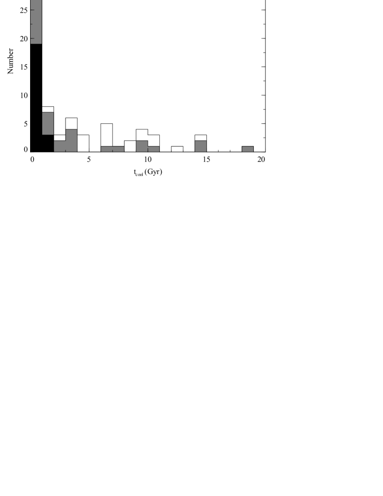
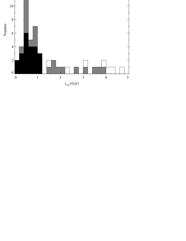
Figure 4: top: The distribution of $t_{\rm cool}$ in the combined cluster sample. bottom: A finer binning of the clusters with a short central $t_{\rm cool}$. The black bars indicate those clusters which harbour clear bubbles, and the grey ones, those with a central radio source.

Fig. 4 shows the distribution of cluster central cooling times. Rather than take the values from the analysis of ROSAT data Peres et al. (1998), we have repeated the extraction of the central cooling time performed here on the BCS sample, on the B55 sample. We note that not all of the clusters in the high redshift end of the BCS sample have been observed with Chandra; in Dunn & Fabian (2006) clusters without short central cooling times or central radio sources were discarded from further analysis, whereas all clusters for which Chandra observations exist have been analysed in this work. As a result the fraction of clusters harbouring bubbles/radio sources as a function of the central cooling time are estimates.

What can be seen from Fig. 4, however, is that radio sources (with or without clear bubbles) are much more common in clusters with central cooling times of $4{\rm\thinspace Gyr}$ or less. In fact there are only 10/24 clusters with $t_{\rm cool}\geq 4{\rm\thinspace Gyr}$ which have central radio sources. In the distribution with finer binning, the peak in the central cooling times appears at around $0.6{\rm\thinspace Gyr}$. In the current combined samples, there appear to be no clusters which harbour clear bubbles and have central cooling times $>1.2{\rm\thinspace Gyr}$. Very few clusters (5/47) with central cooling times shorter than $4{\rm\thinspace Gyr}$ have no evidence for a central radio source (from the NVSS).

Although the two samples combined here have not been created in the same way (lack of non-cool core/non-radio source harbouring clusters in the B55 analysis) there appears to be an excess of clusters which have a cooling time of $\lesssim 1{\rm\thinspace Gyr}$. To take into account the effect of all the clusters in the B55 sample which have not yet been analysed on Fig 4, we look at the distribution of $t_{\rm cool}$ at $>3{\rm\thinspace Gyr}$. The distribution is fairly flat, so even if all the remaining clusters follow this flat distribution, then the “pile-up” of clusters at $t_{\rm cool}<1.2{\rm\thinspace Gyr}$ would still be seen.

An explanation of this pile-up could result from the feedback cycle suggested as a solution to the cooling flow problem. Only once the central cooling time is less than $\sim 1{\rm\thinspace Gyr}$ will the AGN be active and inject energy into the central regions of the cluster and create the tell-tale bubbles. It would depend on whether the AGN activity is gentle and relatively continuous or explosive and intermittent as to what the final state of the cluster would be. An explosive and energetic AGN outburst would increase the ICM temperature, and hence cooling time by a large amount. As a result the next injection event would occur after a long dormant period. However, a gentle injection of energy would only reheat the ICM a small amount, and so the next injection event would take place relatively shortly thereafter.

The large number of clusters at short cooling times, some of which have radio sources but no clear bubbles, implies that the majority of injection events are the “gentle and often” kind; as most clusters with radio sources (dormant AGN?) and bubbles are found with short central cooling times.

Bauer et al. (2005) investigated the cooling time profiles of the Chandra-observed BCS clusters. There are five more clusters in our sample as we use a lower minimum redshift for our sample selection and there have been further observations of BCS clusters. We compare our central cooling times to theirs and find that on average ours are shorter by around a factor 0.7. There are some differences between the data-reduction methods of the two studies. We do use the cluster centroid as calculated by the ciao software as in Bauer et al. (2005), but then visually inspect the annular regions and manually change their location to match the surface brightness peak (12 clusters). We also allow the galactic absorption to be unconstrained in the spectral fitting. Bauer et al. (2005) state that using only the centroid rather than the surface brightness peak could bias their central cooling times up by up to a factor 3.

7.1.2 Heating-Cooling balance

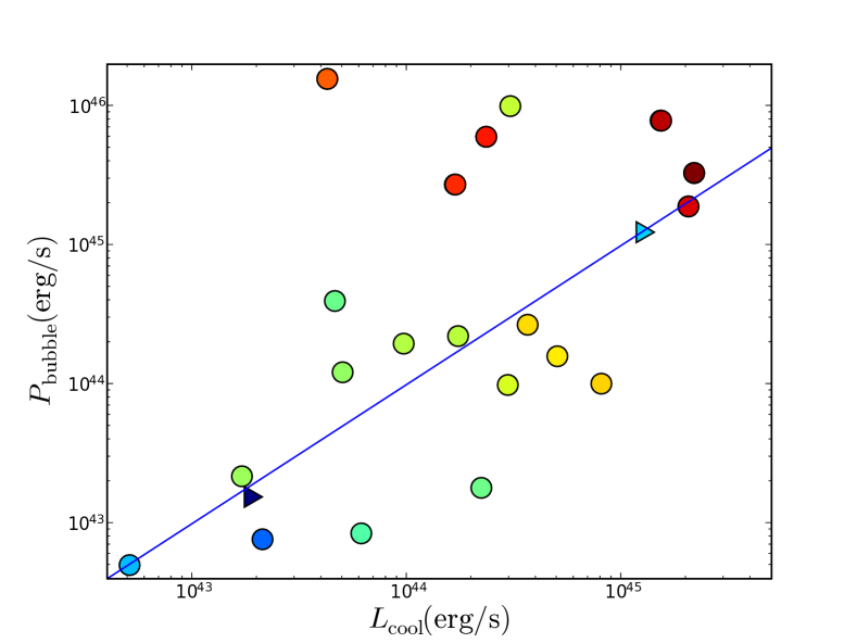
Figure 5: The rate of energy loss via X-ray emission from within the cooling radius of the cluster versus the bubble power from the AGN. These are for the clusters which harbour clear bubbles. The two triangle symbols are for M87 and Perseus where $L_{\rm cool}$ could not be determined from a single ACIS chip. The colour scale is the logarithm of the redshift, blue is low redshift, red is high redshift. The line is for exact balance between $P_{\rm bubble}$ and $L_{\rm cool}$.

We add the six clusters in the BCS sample which harbour clear bubbles to those 16 from the B55 sample and update Fig. 2 of Dunn & Fabian (2006) for the cooling luminosity and the bubble power (Fig. 5). The colour scale shows the redshift of the cluster. The six new clusters are all at the top of the plot in red as they are all at $z>0.15$.

The average distance, as a fraction of the cooling radius, out to which the bubbles can offset the X-ray cooling from the combined sample is $r_{\rm heat}/r_{\rm cool}=0.92\pm 0.11$. The fraction of the X-ray cooling within the cooling radius offset by the action of the AGN is $0.90\pm 0.13$. We ignore those clusters where the bubbles are sufficiently powerful to offset all the cooling within the analysed region, and so only a lower limit on the distance is obtained. Including these clusters gives $r_{\rm heat}/r_{\rm cool}=2.10\pm 0.40$ and the fraction of $20.92\pm 15.11$. Although there are selection effects, especially at the high redshift end of the sample, we can conclude that on average the bubbles counteract the X-ray cooling within the cooling radius.

The problem with this plot is that it shows an instantaneous measure of $L_{\rm cool}$ and $P_{\rm bubble}$ rather than a time average. However for the lower redshift sources it is still reasonable to say that on average the bubble power is sufficient to counteract the X-ray cooling. At the higher redshifts all clusters lie on or above the line of exact balance. Under the assumption that clusters at redshifts of around $0.2-0.3$ are similar to those in the local Universe, we would expect to see some clusters which have bubbles which appear to be insufficient to counteract all the X-ray cooling.

Fig. 6 shows that there is a trend between the average size of a bubble and the X-ray cooling luminosity. The smaller $L_{\rm cool}$, the smaller the detected bubbles. This trend does point to some form of feedback between the X-ray cooling and the kinetic luminosity of the central AGN.

In Fig. 5 there is also a general trend in the redshift of the cluster as the bubble power increases, from bottom left to top right. We do not see any high-redshift, low-power bubbles, which is not unexpected. At high redshifts these bubbles would be too small to detect with the spatial resolution of Chandra. We do, however, see some low-redshift clusters with energetic outbursts – Cygnus A and Perseus. This is also demonstrated in Fig. 6. There are few large bubbles at low redshifts, as a result of the small sampling volume; whereas at high redshifts there are few small bubbles as they would not clearly be resolved.

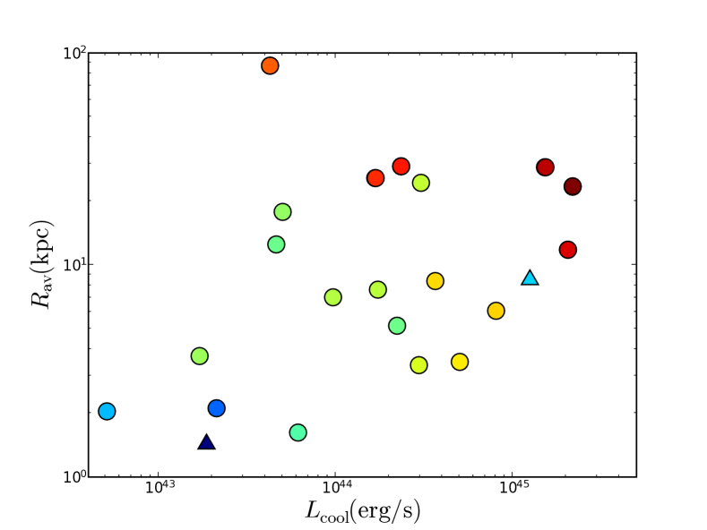
Figure 6: The rate of energy loss via X-ray emission from within the cooling radius of the cluster versus the average bubble size for the cluster. These are for the clusters which harbour clear bubbles. The two triangle symbols are for M87 and Perseus where $L_{\rm cool}$ could not be determined from a single ACIS chip. The colour scale is the logarithm of the redshift, blue is low redshift, red is high redshift.

Figs. 5 and 6 imply that we are missing a number of bubbles, mainly at high redshift, that have not as yet been detected. As they have not as yet been seen by Chandra, then other methods for their detection will have to be developed if their effect on the clusters is going to be analysed in detail, as XEUS will have at best $2\,$arcsec spatial resolution. As can be seen in Fig. 4, most clusters which have short cooling times harbour radio sources, and some have clear bubbles. It could be argued that the natural consequence of an AGN at the centre of a cluster is that, if it is currently producing jets, it produces bubbles and injects energy into the centre of the cluster. The GHz radio emission could then be used as a tracer of the current size of the bubbles, and from this the energy input of the AGN be quantified.

Another interpretation is that the AGN in high redshift clusters are undergoing their first and hence explosive outburst, and that they will, over time, head towards a steady balance between $L_{\rm cool}$ and $P_{\rm bubble}$. However, as Cygnus A and Perseus appear in very similar locations to the high redshift clusters and Perseus has clear evidence for previous outbursts then this explanation is a little uncertain.

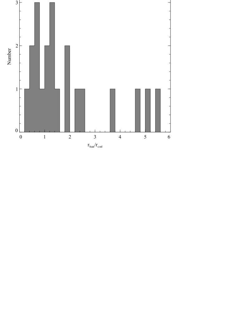
Figure 7: The distribution of radii (as a fraction of the cooling radius) out to which the energy in the bubbles can offset the X-ray cooling for all clusters in the combined sample which have clear bubbles. Hercules A is off the right hand side of this figure ($r_{\rm heat}/r_{\rm cool}=13.1$).

The distribution of radii out to which the energy in the bubbles can offset the X-ray cooling (see Fig. 7) show that a large number of clusters occur around equality with a tail towards “overheating.” As most clusters are close to $r_{\rm heat}/r_{\rm cool}=1$ it is reasonable to assume that even out to $z\sim 0.4$ there is a balance between AGN heating and X-ray cooling, though the caveat of missing small bubbles at high redshifts should be noted.

7.1.3 Duty Cycle

A significant fraction of the clusters in the combined sample have a large heating effect on the cluster. There are two clusters in the B55 sample which have $r_{\rm heat}/r_{\rm cool}>2$ (A2052 & Cygnus A) and there are four in the BCS sample (A115, Hercules A, ZwCl2701 & ZwCl3146). As these outbursts are going to arise in clusters in which some form of heating is expected, the parent sample of these is 34 (20 from B55 and 14 from BCS). Therefore 18 per cent (6/34) of clusters in this sample have extreme outbursts, and hence the duty cycle is also 18 per cent.

7.1.4 Bubble Sizes

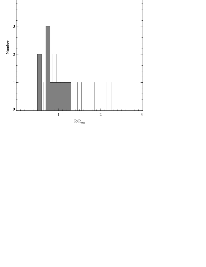
Figure 8: The distribution of the ratio of the average to the “maximum” size of the bubbles. The uncertainties are estimated using a Monte Carlo simulation of the calculations.

We repeat the analysis in Dunn & Fabian (2006) of comparing the observed size of the bubbles to the size expected if they offset all the X-ray cooling within $r_{\rm cool}$. For a detailed description of the method see Section 6.1 of Dunn & Fabian (2006). The “maximum” radius of the bubble is defined as

$$R_{\rm max}=\sqrt{\frac{3\mathcal{C}(L_{\rm cool}/2)}{16\pi p_{\rm th}v_{\rm c_{s}}}},$$ (4)

and is compared to the average radius of the bubble $R_{\rm av}=\sqrt[3]{R_{\rm l}R_{\rm w}^{2}}$. We assume that an AGN will produce two bubbles, hence each will offset $L_{\rm cool}/2$. We use Monte Carlo simulations of the data to allow estimates to be placed on the uncertainties in the distribution. Only clusters with young bubbles were used for this calculation. The distribution is shown in Fig. 8 and still shows a peak at around $R_{\rm av}/R_{\rm max}\sim 0.7$.

The peak has not moved significantly from that found by Dunn & Fabian (2006), which is not surprising as only 3 clusters (6 bubbles) have been added. The explanations for this distribution as outlined in Dunn & Fabian (2006) are therefore all still valid. The bubbles with a small value of $R_{\rm av}/R_{\rm max}$ are small for their host cluster, and so are likely to still be growing. Therefore, it is natural to state that all the bubbles with $R_{\rm av}/R_{\rm max}>1$ are large, i.e. have detached from the core of the cluster and are expanding in the reduced pressure of the higher cluster atmosphere. Some of these large bubbles may involve AGN interactions which are not well described by bubbles, e.g. Hydra A (Nulsen et al., 2005).

As bubbles spend a larger fraction of their lifetime close to their full size rather than growing with small radii, it would be expected to see the majority of clusters with $R_{\rm av}/R_{\rm max}\sim 1$. To shift the peak in the distribution from 0.7 to 1.0 requires $R_{\rm max}$ to reduce. This could be achieved by reducing $L_{\rm cool}$, but this is an unlikely solution. We have already taken a fairly extreme definition for the cooling radius, and it would be more sensible to increase the cooling radius to move it closer to other definitions of cool core clusters.

7.2 Evolution in the Cluster Samples

Comparing the number of clusters requiring heating/harbouring radio sources between the BCS and B55 samples show that they are very similar. The fraction of clusters harbouring radio sources is almost exactly the same for each sample. The fraction of clusters requiring heating is slightly larger for the BCS sample (33 versus 25 per cent). This may be a bias towards Chandra observations of cooling clusters, but may also be a true increase in the fraction of clusters requiring heating.

By combining the clusters in the BCS and B55 samples we have two well defined samples spanning a redshift range of $0.0\leq z\leq 0.37$. However the treatment of the two samples has been different, and so when investigating any changes in the clusters with redshifts we have to redefine the samples so that selection effects do not influence our results.

Dunn & Fabian (2006) did no analysis of clusters in the B55 sample which had no bubbles or central radio source, whereas in the analysis presented here, all clusters which had Chandra observations were studied. To minimise any selection effect we concentrate on clusters with a radio source and/or bubbles.

We have chosen to concentrate on the temperature, entropy and cooling time profiles, and have not split the clusters on whether they harbour clear bubbles or radio sources. The profiles of all 71 clusters are shown in Fig. 9 binned into four redshift bins with equal numbers of clusters in each.

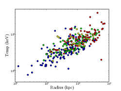
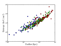
Figure 9: The distributions of the combined sample left: Temperature, centre: Entropy and right: Cooling time. The colour scale shows the redshift of the clusters. The redshifts have been binned into four bins with equal numbers of clusters (18) in each bin (blue $=z\leq 0.0521$, green $=0.0521<z\leq 0.161$, yellow $=0.161<z\leq 0.214$ and red $=z>0.214$).

An initial glance at the temperature profiles gives the impression that the lowest redshift clusters are cooler, with central temperatures to below $1{\rm\thinspace keV}$. However, this is more likely to be a result of resolution rather than redshift evolution. The innermost annulus is going to correspond to a smaller real radius in the nearby clusters as their emission extends over a larger area of the sky and they are also going to be brighter.

The entropy profiles also vary between the lowest and highest redshifts, however this is also most likely the result of resolution.

The cooling time profiles, however, do show some change between the redshift bins which is more likely to be the result of evolution. For a given radius in the cluster the lowest redshift clusters have a longer cooling time than the highest redshift clusters. However, this may still be the result of resolution. In the high redshift clusters the inner regions of the cluster may all be merged together in a single region. This would reduce the average cooling time of this bin. Whereas in the nearby clusters, this region would be split into many separate regions with those with shorter cooling times occuring at smaller radii. The bulk of the scatter in this plot does reduce at higher radii, which is compatible with this argument.

8 Conclusions

We have extended our study of the effect of central AGN in clusters to clusters with $z>0.1$, using the BCS. There are only six clusters which harbour clear bubbles, and on average they overcompensate for the X-ray cooling. These clusters are combined with an updated analysis of those in the B55 cluster sample. The average distance, as a fraction of the cooling radius, out to which the bubbles can offset the X-ray cooling from the combined sample is $r_{\rm heat}/r_{\rm cool}=0.92\pm 0.11$ for clusters where this distance can be reliably determined. Adding in all clusters with bubbles results in $r_{\rm heat}/r_{\rm cool}=2.10\pm 0.40$.

Although it appears as if the AGN bubbles can easily counteract the X-ray cooling within the cooling radius, there is a selection effect, especially at the higher redshifts, which means we are missing small bubbles in the most distant clusters.

Using the result from the BCS bubbles, we calculate the expected size of bubbles within the clusters which harbour radio sources. In three cases (A1068, A1763 and A2204) the predicted bubble sizes and observed radio emission are similar. In some of the clusters the radio source identified in the NVSS is offset to the cluster centre in VLA observations, and so these may be background AGN rather than associated with the cluster. A category of clusters with cool cores, radio sources and no clear bubbles exists in both the B55 and BCS samples. The lack of bubbles is explained by low signal-to-noise ratio in the X-ray images of some but not all of these objects.

The distribution of the central cooling time of the clusters shows that there are no clusters with bubbles which have $t_{\rm cool}>1.2{\rm\thinspace Gyr}$. Also there are only 10/24 clusters with $t_{\rm cool}>4.0{\rm\thinspace Gyr}$ which harbour a central radio source, only 5/47 clusters with $t_{\rm cool}<4.0{\rm\thinspace Gyr}$ have no central radio source.

We investigated the evolution of cluster parameters with redshift and over the range $0.0<z<0.4$ we do not find any significant change. The cooling time profiles show some variation but this can be explained as being the result of the resolution differences as the distances increase.

References

- Adelman-McCarthy & for the SDSS Collaboration (2007) Adelman-McCarthy J. K., for the SDSS Collaboration 2007, arxiv.org/abs/0707.3413
- Arnaud (1996) Arnaud K. A., 1996, in Jacoby G. H., Barnes J., eds, ASP Conf. Ser. 101: Astronomical Data Analysis Software and Systems V XSPEC: The First Ten Years. p. 17
- Bauer et al. (2005) Bauer F. E., Fabian A. C., Sanders J. S., Allen S. W., Johnstone R. M., 2005, MNRAS, 359, 1481
- Bîrzan et al. (2004) Bîrzan L., Rafferty D. A., McNamara B. R., Wise M. W., Nulsen P. E. J., 2004, ApJ, 607, 800
- Blanton et al. (2001) Blanton E. L., Sarazin C. L., McNamara B. R., Wise M. W., 2001, ApJ, 558, L15
- Böhringer et al. (1993) Böhringer H., Voges W., Fabian A. C., Edge A. C., Neumann D. M., 1993, MNRAS, 264, L25
- Burns (1990) Burns J. O., 1990, AJ, 99, 14
- Churazov et al. (2001) Churazov E., Brüggen M., Kaiser C. R., Böhringer H., Forman W., 2001, ApJ, 554, 261
- Churazov et al. (2000) Churazov E., Forman W., Jones C., Böhringer H., 2000, A&A, 356, 788
- Churazov et al. (2002) Churazov E., Sunyaev R., Forman W., Böhringer H., 2002, MNRAS, 332, 729
- Donahue et al. (2006) Donahue M., Horner D. J., Cavagnolo K. W., Voit G. M., 2006, ApJ, 643, 730
- Dunn & Fabian (2006) Dunn R. J. H., Fabian A. C., 2006, MNRAS, 373, 959
- Dunn et al. (2005) Dunn R. J. H., Fabian A. C., Taylor G. B., 2005, MNRAS, 364, 1343
- Ebeling et al. (2000) Ebeling H., Edge A. C., Allen S. W., Crawford C. S., Fabian A. C., Huchra J. P., 2000, MNRAS, 318, 333
- Ebeling et al. (1998) Ebeling H., Edge A. C., Bohringer H., Allen S. W., Crawford C. S., Fabian A. C., Voges W., Huchra J. P., 1998, MNRAS, 301, 881
- Edge et al. (1990) Edge A. C., Stewart G. C., Fabian A. C., Arnaud K. A., 1990, MNRAS, 245, 559
- Fabian et al. (2003) Fabian A. C., Sanders J. S., Allen S. W., Crawford C. S., Iwasawa K., Johnstone R. M., Schmidt R. W., Taylor G. B., 2003, MNRAS, 344, L43
- Fabian et al. (2003) Fabian A. C., Sanders J. S., Crawford C. S., Conselice C. J., Gallagher J. S., Wyse R. F. G., 2003, MNRAS, 344, L48
- Gull & Northover (1973) Gull S. F., Northover K. J. E., 1973, Nature, 244, 80
- Johnstone et al. (2002) Johnstone R. M., Allen S. W., Fabian A. C., Sanders J. S., 2002, MNRAS, 336, 299
- McNamara et al. (2000) McNamara B. R., Wise M., Nulsen P. E. J., David L. P., Sarazin C. L., Bautz M., Markevitch M., Vikhlinin A., Forman W. R., Jones C., Harris D. E., 2000, ApJ, 534, L135
- Mewe et al. (1995) Mewe R., Kaastra J. S., Leidahl D. A., 1995, Legacy, 6, 16
- Nulsen et al. (2005) Nulsen P. E. J., Hambrick D. C., McNamara B. R., Rafferty D., Birzan L., Wise M. W., David L. P., 2005, ApJ, 625, L9
- Nulsen et al. (2005) Nulsen P. E. J., McNamara B. R., Wise M. W., David L. P., 2005, ApJ, 628, 629
- Peres et al. (1998) Peres C. B., Fabian A. C., Edge A. C., Allen S. W., Johnstone R. M., White D. A., 1998, MNRAS, 298, 416
- Peterson & Fabian (2006) Peterson J. R., Fabian A. C., 2006, Physics Reports, 427, 1
- Peterson et al. (2003) Peterson J. R., Kahn S. M., Paerels F. B. S., Kaastra J. S., Tamura T., Bleeker J. A. M., Ferrigno C., Jernigan J. G., 2003, ApJ, 590, 207
- Rafferty et al. (2006) Rafferty D. A., McNamara B. R., Nulsen P. E. J., Wise M. W., 2006, ApJ, 652, 216
- Sanders & Fabian (2002) Sanders J. S., Fabian A. C., 2002, MNRAS, 331, 273
- Voigt & Fabian (2004) Voigt L. M., Fabian A. C., 2004, MNRAS, 347, 1130