Thermodynamics of impurities in the anisotropic Heisenberg spin-1/2 chain

Abstract

The thermodynamics of finite open antiferromagnetic $XXZ$ chains is studied using field theory, Bethe Ansatz and quantum Monte Carlo methods. For the susceptibility a parameter-free result as a function of the number of sites $L$ and temperature $T$ beyond the scaling limit is derived. The limiting cases $T/J\gg 1/L$ (J being the exchange constant), where the boundary correction shows a logarithmically suppressed Curie behaviour, and $T/J\ll 1/L$, where a crossover to the ground state behaviour takes place, are discussed in detail. Based on this analysis we present a simple formula for the averaged susceptibility of a spin-$1/2$ chain doped with non-magnetic impurities. We show that the effective Curie constant has a highly non-trivial temperature dependence and shows scaling in the low-temperature limit. Finally, corrections due to intra- and interchain couplings and implications for experiments on Sr₂Cu_1-xPd_xO_3+δ and related compounds are discussed.

1 Introduction

The spin-1/2 Heisenberg chain is probably the first and most studied example of a strongly correlated quantum system. The first foundations towards exact solutions date back to the early days of quantum mechanics [1] and large scale numerical simulations were already performed in the early sixties [2]. Due to the interesting behaviour of this simple model and the connection with many low-dimensional antiferromagnetic materials, the spin-1/2 chain is still heavily studied today. Some of the most fundamental properties, such as the exact amplitude of the power-law correlation functions [3, 4, 5] and the full temperature behaviour of the susceptibility [6, 4], have only been established after the discovery of high temperature superconductivity has lead to renewed interest in low-dimensional antiferromagnetism. More recently, corrections from impurities and boundaries have come into focus [7, 8, 9, 10, 11, 12, 13, 14, 15, 16, 17, 18, 19, 20, 21, 22, 23, 24, 25, 26], which will also be the topic of this paper.

Boundary thermodynamics are especially relevant for experiments [27, 28, 29, 30, 31] since even the most carefully prepared samples contain imperfections which effectively cut the chains, and corrections to the thermodynamic limit become especially large at low temperatures. In order to analyse the pure and the impurity contributions it is useful to define the finite size corrections

$$\delta F_{FS}(L)=F(L)-Lf_{\mbox{\tiny bulk}}\;\;\mbox{and}\;\;\delta\chi_{FS}(L)=\chi(L)-L\chi_{\mbox{\tiny bulk}}$$ (1.1)

where $F(L)$ ($\chi(L)$) is the total free energy (susceptibility) of a system with $L$ sites and $f_{\mbox{\tiny bulk}}$ ($\chi_{\mbox{\tiny bulk}}$) is the free energy (susceptibility) per site of an infinite pure system. In the limit of $L\to\infty$, $\delta F_{FS}$ and $\delta\chi_{FS}$ become $L$-independent thermodynamic boundary contributions, which will be denoted by $F_{B}$ and $\chi_{B}$ and discussed in detail later on. However, in general $L$ will also take on small values in experimental systems according to a random distribution.

It is well understood that finite chains with an odd number of sites $L$ have doublet ground states, which leads to a diverging Curie susceptibility at temperatures below the first excitation energy $T/J\ll 1/L$ [7]. Recently, it has been established that the boundary susceptibility $\chi_{B}(T)\equiv\delta\chi_{FS}(T,L\to\infty)$ is also divergent in the limit $T\to 0$, albeit with a Curie factor which has a logarithmic temperature dependence [10, 11]. For experimental systems it is desirable to know the complete crossover between the two limits, which has to be averaged according to a random distribution. If the impurity concentration is $p$ and we assume a Poisson distribution, i.e., that the impurity positions are uncorrelated, then the average susceptibility becomes [12, 26]

$$\chi_{p}=p^{2}\sum_{L=0}^{\infty}(1-p)^{L}\chi(L)=(1-p)\chi_{\mbox{\tiny bulk}}+p\ \delta\bar{\chi}_{FS},$$ (1.2)

where $\delta\bar{\chi}_{FS}=p\sum_{L}(1-p)^{L}\delta\chi_{FS}(L)$ and we have assumed that each impurity effectively removes one site. The typical approximation in experimental papers to estimate the impurity concentration by the low-temperature Curie tail corresponds to setting $\delta\bar{\chi}_{FS}=1/(8T)$ (assuming that each chain segment with odd length acts effectively like a free spin-$1/2$). This, however, does not capture the full complexity of the problem and might, in particular, lead to an underestimate of the impurity concentration by an order of magnitude.

Several experiments have been studying the prototypical spin-$1/2$ chain compound Sr₂CuO₃ [27, 28, 30, 31] and the doped system Sr₂Cu_1-xPd_xO₃ [29] where palladium serves as a non-magnetic impurity. The analysis of the susceptibility even in the undoped system has been hampered by large Curie-like contributions at low temperatures making a detailed test of the theoretical predictions for the susceptibility of the pure system [6] difficult. In [27, 28] it has been shown that these contributions can be largely suppressed by annealing the samples. It therefore has been suggested that the Curie-like contribution is caused by excess oxygen. Each excess oxygen atom would then dope two holes into the chain. A detailed theoretical analysis of the susceptibility data [26] has shown that it seems to be possible to consistently describe the data by assuming that these holes are basically immobile and therefore effectively cut the chain into finite segments. A more detailed understanding of these experiments is desirable because it might also shed some light on the general issue of oxygen doping in cuprates, and in particular, in the high-temperature superconductors.

Our paper is organised as follows: In section 2 the effective field theory description of the spin-1/2 chain is reviewed. In section 3 we calculate the free energy for an open anisotropic Heisenberg chain of finite length at finite temperature by field theory methods beyond the scaling limit. Next, we consider the limit $L\to\infty$ with $T/J$ fixed in section 4 where $\delta F_{FS}$ and $\delta\chi_{FS}$ as defined in (1.1) become well defined boundary quantities. In section 5 we then discuss separately the isotropic model which is the most interesting case from an experimental point of view. In the limit, $T/J\ll 1/L$, considered in section 6, a crossover to the ground state limit takes place and logarithmic corrections to the scaling limit result are studied in detail. In section 7 we then derive a simple formula which can be used to fit the experimentally measured averaged susceptibility $\chi_{p}$. We also discuss here the temperature dependence of the effective Curie constant $C\sim T\delta\bar{\chi}_{FS}$. In any real material there will be residual couplings bridging between the chain segments (intrachain couplings) as well as interchain couplings which will usually lead to some sort of magnetic order at low temperatures. The effect of such couplings will be discussed in section 8. A comparison between our theoretical predictions and experiments on Sr₂Cu_1-xPd_xO₃ [29] is presented in section 9. Finally, we conclude and give a short summary in section 10.

2 Effective field theory for the spin-1/2 chain

The Hamiltonian for the spin-1/2 Heisenberg chain with open boundaries in an external magnetic field $h$ is given by,

$$H=J\sum_{i=1}^{L-1}[S_{i}^{x}S_{i+1}^{x}+S_{i}^{y}S_{i+1}^{y}+\Delta S_{i}^{z}S_{i+1}^{z}]-h\sum_{i=1}^{L}S_{i}^{z},$$ (2.1)

with $J>0$ for an antiferromagnetic system. Here, we have introduced an exchange anisotropy $\Delta$ which is convenient to obtain a low-energy effective theory by bosonisation. Such a description is by now well established [32, 4] and numerical simulations have shown its applicability for $L\gtrsim 10$ and low temperatures $T\lesssim 0.1J$, which is also the most interesting regime for experiments. In the massless case, $-1<\Delta\leq 1$, the low energy fixed point of (2.1) is the Tomonaga-Luttinger liquid, which belongs to the universality class of the Gaussian theory with the central charge $c=1$.

Ignoring irrelevant operators the Hamiltonian is then equivalent to a free boson model

$$H_{0}=\frac{v}{2}\int_{0}^{La^{\prime}}\!\!dx\;[\Pi^{2}+(\partial_{x}\phi)^{2}]-h\sqrt{\frac{K}{2\pi}}\int^{La^{\prime}}_{0}\!\!dx\;\partial_{x}\phi,$$ (2.2)

where $a^{\prime}$ is the lattice constant. $\phi$ is a bosonic field and $\Pi=v^{-1}\partial_{t}\phi$ the conjugate momentum obeying the standard commutation rule $[\phi(x),\Pi(x^{\prime})]=\mbox{i}\delta(x-x^{\prime})$. The dependence of the Luttinger parameter $K$ on anisotropy $\Delta$ is known exactly from Bethe Ansatz

$$K=[1-\frac{1}{\pi}\cos^{-1}(\Delta)]^{-1},$$ (2.3)

as well as the velocity [33]

$$v=\frac{JK\sin(\pi/K)}{2(K-1)}a^{\prime}\;.$$ (2.4)

In the following we will set the lattice constant $a^{\prime}\equiv 1$. Factors of $a^{\prime}$ can be easily restored in the final results by dimensional analysis. Using the mode expansion for open boundary conditions (OBCs)

$$\phi(x,t) = \sqrt{\frac{\pi}{8K}}+\sqrt{\frac{2\pi}{K}}S_{z}\frac{x}{L}+\sum_{n=1}^{\infty}\frac{\sin\left(\pi nx/L\right)}{\sqrt{\pi n}}\left(\mbox{e}^{-i\pi n\frac{vt}{L}}a_{n}+\mbox{e}^{i\pi n\frac{vt}{L}}a_{n}^{\dagger}\right)$$ (2.5)

the Hamiltonian can also be expressed in terms of bosonic creation and annihilation operators $a_{n}$

$$H_{0}=\frac{\pi v}{LK}S_{z}^{2}+\frac{\pi v}{L}\sum_{n=1}^{\infty}n(a_{n}^{\dagger}a_{n}^{~{}}+1/2)-hS_{z}.$$ (2.6)

The zero mode operator $S_{z}=\sqrt{\frac{K}{2\pi}}\int^{L}_{0}dx\ \partial_{x}\phi$ measures the total magnetisation of the chain and is therefore quantised to take on integer values for chains with an even number of sites $L$ and half-integer values for odd $L$.

Up to this point the effective model is easily solvable exactly. The partition function can be obtained directly by summing over all eigenvalues

$$Z_{0} = \sum_{S_{z}}e^{-\frac{\pi v}{KLT}S_{z}^{2}+\frac{h}{T}S_{z}}\prod_{n=1}^{\infty}\left[2\sinh\left(\frac{\pi v}{2LT}n\right)\right]^{-1}$$

$$= \theta\left(e^{-\frac{\pi v}{KLT}},-i\frac{h}{2T}\right)\prod_{n=1}^{\infty}\left[2\sinh\left(\frac{\pi v}{2LT}n\right)\right]^{-1}$$

where $\theta(q,u)$ is the elliptic theta function of the third kind $\theta=\theta_{3}(q,u)=\sum_{n=-\infty}^{\infty}q^{n^{2}}e^{i2nu}$ for integer $S_{z}$ (even $L$) and of the second kind $\theta=\theta_{2}(q,u)=\sum_{n=-\infty}^{\infty}q^{(n+1/2)^{2}}e^{i(2n+1)u}$ for half-integer $S_{z}$ (odd $L$).

The free energy per site is then given by

$$f_{0}=-\frac{T}{L}\left\{\ln\theta\left(e^{-\frac{\pi v}{KLT}},-i\frac{h}{2T}\right)-\sum_{n=1}^{\infty}\ln\left[2\sinh\left(\frac{\pi v}{2LT}n\right)\right]\right\}\;.$$ (2.8)

and the susceptibility by

$$\chi_{0} = -\frac{\partial^{2}}{\partial h^{2}}\bigg{|}_{h=0}f_{0}=\frac{1}{LT}\frac{\sum_{S_{z}}S_{z}^{2}e^{-\frac{\pi v}{KLT}S_{z}^{2}}}{\sum_{S_{z}}e^{-\frac{\pi v}{KLT}S_{z}^{2}}}=-\frac{1}{4LT}\frac{\partial^{2}}{\partial u^{2}}\bigg{|}_{u=0}\ln\theta\left(e^{-\frac{\pi v}{KLT}},u\right)$$ (2.9)

Note, that $\chi_{0}$ has a simple scaling form as a function of $LT$ [7]. The following limiting cases are of interest

$$\chi_{0} = \left\{\begin{array}[]{ll}\frac{2}{LT}\exp\left[-\frac{\pi v}{KLT}\right]&LT/v\to 0,\;\mbox{$L$ even}\\[5.69046pt] \frac{1}{4TL}&LT/v\to 0,\;\mbox{$L$ odd}\\[5.69046pt] \frac{K}{2\pi v}\pm\frac{2K^{2}}{v}\frac{LT}{v}\exp\left(-\pi K\frac{LT}{v}\right)&LT/v\to\infty\;\;.\end{array}\right.$$ (2.13)

Here the plus (minus) sign in front of the second term in the last line corresponds to L odd (even), respectively. This term represents the leading finite size correction to the thermodynamic limit result $\chi_{0}=K/(2\pi v)$. In the limit $T/v\ll 1/L$ on the other hand, the susceptibility for a chain of fixed even length vanishes exponentially because it locks into its singlet ground state, whereas $\chi_{0}$ for a chain of odd length exhibits a $1/T$ divergence due to its doublet ground state.

If we were only interested in the qualitative behaviour we could stop at Eq. (2.9), which in some cases is sufficient for agreement with experimental data [8]. However, the comparison with quantum Monte Carlo data in Fig. 1 clearly shows sizeable deviations from the scaling limit result.

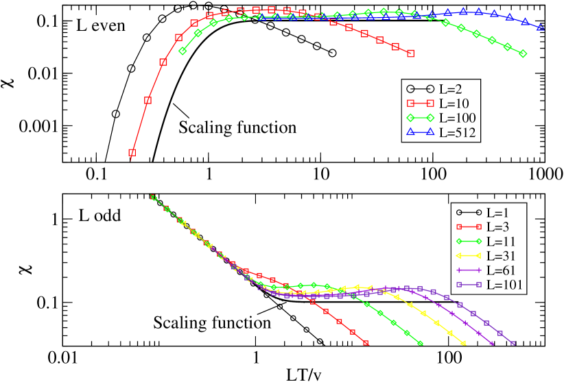
Figure 1: The scaling behaviour of the susceptibility as a function of $LT/v$ in Eq. (2.9) for the isotropic case $\Delta=1,\ K=1,\ v=\pi/2$ (black solid lines) for $L$ even (upper panel) and $L$ odd (lower panel), respectively. The symbols denote quantum Monte Carlo data for chains of different lengths, obtained within the SSE loop algorithm framework  [34].

For more accurate predictions and the understanding of impurity corrections it is therefore necessary to take the leading irrelevant operator into account, which is given by [32, 4]

$$\delta H=\lambda\int_{0}^{L}dx\,\cos(\sqrt{8\pi K}\phi).$$ (2.14)

The operator $\cos(\sqrt{8\pi K}\phi)$ has scaling dimension $2K$ so that this perturbation becomes marginally irrelevant at the isotropic point $K=1$. The next-leading irrelevant operators at zero magnetic field are of the form $\sim(\partial_{x}\phi)^{4}$ and will be neglected in the following unless it is explicitly stated otherwise. The coupling strength $\lambda$ has been obtained exactly by Bethe ansatz [4] and is given in a particular normalisation as discussed in detail later on by

$$\lambda=\frac{K\Gamma(K)\sin\pi/K}{\pi\Gamma(2-K)}\left[\frac{\Gamma\left(1+\frac{1}{2K-2}\right)}{2\sqrt{\pi}\Gamma\left(1+\frac{K}{2K-2}\right)}\right]^{2K-2}\;.$$ (2.15)

At the isotropic point $\Delta=1$ ($K=1$) where the interaction (2.14) becomes marginal the amplitude $\lambda$ as given by (2.15) vanishes. Here $\lambda$ has to be replaced by an RG-improved coupling constant, and, in general, becomes a function of the different scales $T,L$, and $h$. This will be discussed in detail in section 5.

Generally, in systems with boundaries, there may be boundary operators in addition to bulk interactions. However, as was pointed out in Ref. [13], in the absence of symmetry-breaking external fields at boundaries, there are no relevant boundary operators for the anisotropic Heisenberg chain. The leading irrelevant boundary operator has scaling dimension $2$ and is of the form $\delta(x)(\partial_{x}\phi)^{2}$ [7]. This operator effectively leads to a replacement of the length $L$ of the system by some effective length $L^{\prime}$ as will be discussed in the next section.

3 Thermodynamics for a finite chain beyond the scaling limit

To calculate the free energy and susceptibility for an open $XXZ$ chain with length $L$ at finite temperature $T$ beyond the scaling limit (2.8,2.9), the leading correction (2.14) has to be taken into account. As this operator is irrelevant for $0\leq\Delta<1$ it is sufficient to use perturbation theory. This anisotropic regime will be considered here.

In first order perturbation theory we obtain

$$\delta f_{1}=\frac{\lambda}{L}\int_{0}^{L}dx\left\langle\cos\left(\sqrt{8\pi K}\phi\right)\right\rangle\;.$$ (3.1)

This term has been considered in Refs. [10, 11, 25] in the limit $L\to\infty$ and gives the leading contribution to the boundary free energy. A bulk contribution, i.e. a term which scales linearly with $L$ at large $L$, occurs in second order perturbation theory in $\lambda$ [4] (see also A).

The expectation value can be split into an $S_{z}$-part (zero mode) and an oscillator part

$$\left\langle\exp\left(\pm\mbox{i}\sqrt{8\pi K}\phi\right)\right\rangle = \left\langle\exp\left(\pm\mbox{i}\sqrt{8\pi K}\phi\right)\right\rangle_{\mbox{\tiny$S_{z}$}}\left\langle\exp\left(\pm\mbox{i}\sqrt{8\pi K}\phi\right)\right\rangle_{\mbox{\tiny osc.}}$$ (3.2)

$$\!\!\!\!\!\!\!\!\!\!\!\!\!\!\!\!\!\!\!\!\!\!\!\!\!\!\!= \!\!\!\!\!\!\!\!\!\!\!\!\!\!\left\langle\exp\left(\pm\mbox{i}\sqrt{8\pi K}\phi\right)\right\rangle_{\mbox{\tiny$S_{z}$}}\exp\left(-4\pi K\langle\phi\phi\rangle_{\mbox{\tiny osc.}}\right)\,,$$

where we used the cumulant theorem for bosonic modes in the second line. Using the mode expansion (2.5) we find

$$\left\langle\exp\left(\pm\mbox{i}\sqrt{8\pi K}\phi\right)\right\rangle_{\mbox{\tiny$S_{z}$}}=\frac{\sum_{S_{z}}\mbox{e}^{\pm\frac{4\pi iS_{z}x}{L}}\mbox{e}^{-\frac{\pi vS_{z}^{2}}{KLT}}\mbox{e}^{\frac{hS_{z}}{T}}}{\sum_{S_{z}}\mbox{e}^{-\frac{\pi vS_{z}^{2}}{KLT}}\mbox{e}^{\frac{hS_{z}}{T}}}$$ (3.3)

and

$$\langle\phi\phi\rangle_{\mbox{\tiny osc.}}=\sum_{l=1}^{\infty}\frac{\sin^{2}(\pi lx/L)}{\pi l}\left(1+\frac{2}{\mbox{e}^{\pi vl/(TL)}-1}\right)\;.$$ (3.4)

The zero temperature part of (3.4) is divergent and we have to introduce a cutoff $\alpha$ with dimensions of length, of order a lattice spacing. Doing so and using $\sum_{l=1}^{\infty}z^{l}/l=-\ln(1-z)$ for $|z|<1$ leads to

$$\sum_{l=1}^{\infty}\frac{\sin^{2}(\pi lx/L)}{\pi l}\mbox{e}^{-\alpha\pi l/L}=-\frac{1}{2\pi}\ln(\alpha\pi/L)$$

$$+ \frac{1}{4\pi}\ln\left[\left(1-\mbox{e}^{2\pi ix/L}\mbox{e}^{-\alpha\pi/L}\right)\left(1-\mbox{e}^{-2\pi ix/L}\mbox{e}^{-\alpha\pi/L}\right)\right]\;.$$

Writing the exponential factor of the finite temperature part in Eq. (3.4) as a geometric series we find

$$\frac{1}{\pi}\sum_{l=1}^{\infty}\sum_{n=1}^{\infty}\left(\frac{1}{l}-\frac{\mbox{e}^{2\pi ixl/L}+\mbox{e}^{-2\pi ixl/L}}{2l}\right)\mbox{e}^{-\pi vnl/(TL)}$$

$$= \frac{1}{\pi}\sum_{n=1}^{\infty}\left\{-\ln\left(1-\mbox{e}^{-\pi vn/(TL)}\right)\right.$$

$$+ \left.\frac{1}{2}\ln\left[\left(1-\mbox{e}^{2\pi ix/L}\mbox{e}^{-\pi vn/(TL)}\right)\left(1-\mbox{e}^{-2\pi ix/L}\mbox{e}^{-\pi vn/(TL)}\right)\right]\right\}\;.$$

Combining Eqs. (3.4, 3, 3) gives

$$\exp\left\{-4\pi K\langle\phi\phi\rangle_{\mbox{\tiny osc.}}\right\}$$

$$= \left(\frac{\alpha\pi}{L}\right)^{2K}\left[\left(1-\mbox{e}^{2\pi ix/L}\mbox{e}^{-\alpha\pi/L}\right)\left(1-\mbox{e}^{-2\pi ix/L}\mbox{e}^{-\alpha\pi/L}\right)\right]^{-K}$$

$$\times \prod_{n=1}^{\infty}\left[\frac{\left(1-\mbox{e}^{2\pi ix/L}\mbox{e}^{-\pi vn/(TL)}\right)\left(1-\mbox{e}^{-2\pi ix/L}\mbox{e}^{-\pi vn/(TL)}\right)}{\left(1-\mbox{e}^{-\pi vn/(TL)}\right)^{2}}\right]^{-2K}$$

$$= \left(\frac{2\alpha\pi}{L}\right)^{2K}\left[\left(1-\mbox{e}^{2\pi ix/L}\mbox{e}^{-\alpha\pi/L}\right)\left(1-\mbox{e}^{-2\pi ix/L}\mbox{e}^{-\alpha\pi/L}\right)\right]^{-K}$$

$$\times \sin^{2K}\left(\frac{\pi x}{L}\right)\frac{\eta^{6K}\left(\mbox{e}^{-\pi v/(TL)}\right)}{\theta_{1}^{2K}\left(\frac{\pi x}{L},\mbox{e}^{-\pi v/(2TL)}\right)}$$

In the last step we have written the oscillator part in terms of the Dedekind eta-function

$$\eta(w)=w^{1/24}\prod_{n=1}^{\infty}\left(1-w^{n}\right)$$ (3.8)

and the elliptic theta-function of the first kind

$$\theta_{1}(u,q)=2q^{1/4}\sin u\prod_{n=1}^{\infty}\left(1-2q^{2n}\cos 2u+q^{4n}\right)\left(1-q^{2n}\right)\;.$$ (3.9)

From (3.3) and (3) we now directly obtain the correction to the scaling form of the free energy (2.8)

$$\delta f_{1} = 2\tilde{\lambda}\left(\frac{\pi}{L}\right)^{2K}\!\!\eta^{6K}\left(\mbox{e}^{-\frac{\pi v}{TL}}\right)\int_{0}^{1/2}\!\!dy\,\frac{\tilde{g}\left(y,\mbox{e}^{-\frac{\pi v}{KLT}},e^{\frac{h}{T}}\right)}{\theta_{1}^{2K}\left(\pi y,\mbox{e}^{-\frac{\pi v}{2TL}}\right)}$$ (3.10)

$$\times 2^{2K}\sin^{2K}\left(\pi y\right)\left[\left(1-\mbox{e}^{2\pi iy}\mbox{e}^{-\alpha\pi/L}\right)\times\mbox{h.c.}\right]^{-K}$$

with

$$\tilde{g}\left(y,q,w\right) = \frac{\sum_{S_{z}}\cos(4\pi S_{z}y)q^{S_{z}^{2}}w^{S_{z}}}{\sum_{S_{z}}q^{S_{z}^{2}}w^{S_{z}}}$$ (3.11)

and $\tilde{\lambda}=\alpha^{2K}\lambda$. It is actually $\tilde{\lambda}$ which is given by Eq. (2.15), but we will identify both in the following. Note, that the integral in (3.10) is convergent for $K<1/2$. In this case the cutoff $\alpha$ can be dropped in the last line in (3.10) which then becomes equal to one. For $K>1/2$ we can isolate the cutoff independent part by subtracting the Taylor expand of the integrand up to sufficient order in $y$, and then take $\alpha\to 0$.

We will discuss this in detail in the following for the correction to the susceptibility which is readily obtained from (3.10) and reads

$$\delta\chi_{1} = \frac{2\lambda}{T^{2}}\left(\frac{\pi}{L}\right)^{2K}\!\!\eta^{6K}\left(\mbox{e}^{-\frac{\pi v}{TL}}\right)\int_{0}^{1/2}\!\!\!\!\!\!dy\,\frac{g_{0}\left(y,\mbox{e}^{-\frac{\pi v}{KLT}}\right)}{\theta_{1}^{2K}\left(\pi y,\mbox{e}^{-\frac{\pi v}{2TL}}\right)}$$ (3.12)

$$\times 2^{2K}\sin^{2K}\left(\pi y\right)\left[\left(1-\mbox{e}^{2\pi iy}\mbox{e}^{-\alpha\pi/L}\right)\times\mbox{h.c.}\right]^{-K}$$

where we have defined a new function for the zero mode part

$$g_{0}\left(y,q\right) = -\frac{\sum_{S_{z}}S_{z}^{2}\cos(4\pi S_{z}y)q^{S_{z}^{2}}}{\sum_{S_{z}}q^{S_{z}^{2}}}+\frac{\left(\sum_{S_{z}}\cos(4\pi S_{z}y)q^{S_{z}^{2}}\right)\left(\sum_{S_{z}}S_{z}^{2}q^{S_{z}^{2}}\right)}{\left(\sum_{S_{z}}q^{S_{z}^{2}}\right)^{2}}\,.$$ (3.13)

Because of the modified zero mode part, the integral is now convergent for $K<3/2$ and the last line can be set equal to one in this case again. For $3/2<K<5/2$ we can obtain a convergent integral, i.e. the cutoff independent part, by subtracting just the first non-vanishing order in a Taylor expand in $y$ and setting $\alpha\to 0$ then. Noting that

$$\lim_{y\to 0}\frac{2^{2K}\sin^{2K}\left(\pi y\right)\eta^{6K}\left(\mbox{e}^{-\frac{\pi v}{TL}}\right)}{\theta_{1}^{2K}\left(\pi y,\mbox{e}^{-\frac{\pi v}{2TL}}\right)}=1$$ (3.14)

the cutoff independent part of (3.12) for $3/2<K<5/2$ is given by

$$\!\!\!\!\!\!\!\!\!\!\!\!\!\!\!\!\!\!\!\!\delta\chi_{1} = \frac{2\lambda}{T^{2}}\left(\frac{\pi}{L}\right)^{2K}\!\!\!\!\int_{0}^{1/2}\!\!\!\!\!\!dy\left\{\frac{\eta^{6K}\left(\mbox{e}^{-\frac{\pi v}{TL}}\right)g_{0}\left(y,\mbox{e}^{-\frac{\pi v}{KLT}}\right)}{\theta_{1}^{2K}\left(\pi y,\mbox{e}^{-\frac{\pi v}{2TL}}\right)}\right.-\left.\frac{2g_{2}\left(\mbox{e}^{-\frac{\pi v}{KLT}}\right)}{(2\pi y)^{2K-2}}\right\}$$ (3.15)

where

$$g_{2}\left(q\right)=\frac{\sum_{S_{z}}S_{z}^{4}q^{S_{z}^{2}}}{\sum_{S_{z}}q^{S_{z}^{2}}}-\frac{\left(\sum_{S_{z}}S_{z}^{2}q^{S_{z}^{2}}\right)^{2}}{\left(\sum_{S_{z}}q^{S_{z}^{2}}\right)^{2}}\,.$$ (3.16)

Now we have to add again the first non-vanishing order in the Taylor expand in $y$ but this time we keep the cutoff $\alpha$ giving us the non-universal contribution

$$\delta\chi_{1}^{nu}=\frac{16\pi^{2}\lambda}{T^{2}}\left(\frac{\pi}{L}\right)^{2K}\!\!\!\!g_{2}\left(\mbox{e}^{-\frac{\pi v}{KLT}}\right)\int_{0}^{1/2}\!\!\!\!\!\!\frac{y^{2}\,dy}{\left[(2\pi y)^{2}+\left(\frac{\alpha\pi}{L}\right)^{2}\right]^{K}}\;.$$ (3.17)

Shifting the upper boundary of integration to infinity, we can evaluate the integral and find

$$\delta\chi_{1}^{nu}=\frac{\pi^{3/2}\lambda}{2T^{2}L^{3}}g_{2}\left(\mbox{e}^{-\frac{\pi v}{KLT}}\right)\frac{\Gamma(K-3/2)}{\Gamma(K)}\alpha^{3-2K}\;.$$ (3.18)

The other non-universal correction stems from the irrelevant boundary operator $\sim\delta(x)(\partial_{x}\phi)^{2}$. Including this term into the Hamiltonian (2.2) is equivalent to replacing the length by some effective length $L\to L^{\prime}\equiv L+a$. Using this effective length in the exponentials in (2.9) and expanding to lowest order in $a$ yields

$$\delta\chi_{2}=\frac{\pi va}{KT^{2}L^{3}}g_{2}\left(\mbox{e}^{-\frac{\pi v}{KLT}}\right)\;.$$ (3.19)

We see that this correction has the same form as (3.18). We therefore can consider $a$ in (3.19) as an effective parameter incorporating both corrections. In the thermodynamic limit $g_{2}\left(\mbox{e}^{-\pi v/(KLT)}\right)\to K^{2}T^{2}L^{2}/(2\pi^{2}v^{2})$ and $\delta\chi_{2}\to Ka/(2\pi vL)$. In this limit we can compare the field theory result with a recent calculation of the boundary susceptibility based on the Bethe ansatz [24, 25] leading to

$$a=2^{-1/2}\sin\left[\pi K/(4K-4)\right]/\cos\left[\pi/(4K-4)\right]\;.$$ (3.20)

Eq. (3.12) for $K<3/2$ or (3.15) for $K>3/2$ taken together with (3.19, 3.20) is therefore a parameter-free result for the susceptibility of an open chain with length $L$ at temperature $T$ to first order in the Umklapp scattering. In [26] it has been shown by comparing with quantum Monte-Carlo data that this formula does describe the susceptibility of open chains for $L\gtrsim 10$ and $T/J\lesssim 0.1$ very well. Note, however, that the parameter $a$ in (3.20) has poles at $K=(4n+3)/(4n+2)$, $n=0,1,2,\cdots$ with an accumulation point at $K=1$. At these special points a contribution stemming from a different irrelevant operator will also be divergent while having the same dependence on temperature and length and both terms taken together will give something finite. In the limit $L\to\infty$ this has been investigated in detail in Ref. [25]. In particular, it has been shown in this limit that at $K=3/2$ ($\Delta=1/2$) the two contributions (3.12) and (3.19) “conspire” to produce a logarithmic temperature dependence of the boundary susceptibility.

4 Boundary contributions: The limit $L\to\infty$ with $T/J$ fixed

The boundary free energy can be obtained directly by starting with the integral (3.1) in the limit $L\to\infty$ and using either boundary conformal field theory [10] or the thermodynamic limit result for the correlation function [11, 25]. Here we want to show that our more general result (3.10) for a finite chain reduces to the known result in the thermodynamic limit. First, we consider the limit $L\to\infty$ for the function $\tilde{g}$ in (3.11). For $x\ll L$ we can replace the sums by integrals and find

$$\tilde{g}\left(\frac{x}{L},\mbox{e}^{-\frac{\pi v}{KLT}},e^{\frac{h}{T}}\right) \approx \mbox{e}^{-\frac{4\pi KT}{vL}x^{2}}\cos\left(\frac{2Khx}{v}\right)\stackrel{{\scriptstyle L\to\infty}}{{\to}}\cos\left(\frac{2Khx}{v}\right)$$ (4.1)

We see that $\tilde{g}$ decays fast away from the boundary. If $x\sim L$, on the other hand, we can set $x\to L-x$ and because $S_{z}$ is integer or half-integer $\cos(4\pi S_{z}(L-x)/L)=\cos(4\pi S_{z}x/L)$ and we get exactly the same result again. In the thermodynamic limit the two boundaries therefore become independent and each of them yields the same contribution. To perform the thermodynamic limit for the oscillator part it is easiest to go back to Eqns. (3.4, 3, 3). We want to consider here only the case $K<3/2$. In this case the cutoff in the second line of (3) can be dropped leading to

$$\sum_{l=1}^{\infty}\frac{\sin^{2}(\pi lx/L)}{\pi l}\mbox{e}^{-\alpha\pi l/L} \approx \frac{1}{2\pi}\ln\left\{\frac{L\left(2-2\cos\left(\frac{2\pi x}{L}\right)\right)^{1/2}}{\alpha\pi}\right\}$$ (4.2)

$$\stackrel{{\scriptstyle L\to\infty}}{{\to}} \frac{1}{2\pi}\ln\left\{\frac{2x}{\alpha}\right\}\;.$$

Note that $\alpha$ will later be absorbed again into the coupling constant $\lambda\to\tilde{\lambda}=\alpha^{2K}\lambda$. For the finite temperature part we can replace the momentum sum in (3) by an integral, allowing us to perform the sum over $n$ (“Matsubara sum”) exactly

$$\frac{1}{\pi}\sum_{n=1}^{\infty}\sum_{l=1}^{\infty}\left(\frac{1}{l}-\frac{\mbox{e}^{2\pi ixl/L}+\mbox{e}^{-2\pi ixl/L}}{2l}\right)\mbox{e}^{-\pi vnl/(TL)}$$ (4.3)

$$\to \frac{1}{\pi}\sum_{n=1}^{\infty}\int_{0}^{\infty}dk\,\left(\frac{1}{k}-\frac{\mbox{e}^{2ikx}+\mbox{e}^{-2ikx}}{2k}\right)\mbox{e}^{-\frac{vk}{T}n}$$

$$= \frac{1}{2\pi}\sum_{n=1}^{\infty}\ln\left(1+\frac{4T^{2}x^{2}}{n^{2}v^{2}}\right)=\frac{1}{2\pi}\ln\left(\frac{v}{2\pi Tx}\sinh\left(\frac{2\pi Tx}{v}\right)\right)\;.$$

Thus we find in the thermodynamic limit

$$F_{B}=L\,\delta f_{1}(L\to\infty)=2\lambda\int_{0}^{\infty}\!\!\!\!dx\;\frac{\cos\left(\frac{2Khx}{v}\right)}{\left[\frac{v}{\pi T}\sinh\left(\frac{2\pi Tx}{v}\right)\right]^{2K}}\;.$$ (4.4)

This is the result obtained previously by boundary conformal field theory [10] and by using the result for the correlation function in the thermodynamic limit in (3.1) [11, 25]. For $K<3/2$ ($\Delta>1/2$) the integral is convergent and yields [25]

$$F_{B}=\lambda\;{\rm Re}[B(K+i\frac{Kh}{2\pi T},1-2K)]\left(\frac{2\pi T}{v}\right)^{2K-1},$$ (4.5)

where $B(x,y)=\Gamma(x)\Gamma(y)/\Gamma(x+y)$. For $K>3/2$ the integral (4.4) is divergent and a cutoff has to be introduced again. Then, the cutoff independent part of the integral is still given by (4.5) whereas the cutoff dependent terms are regular in $h,T$ [25]. In the following discussion we will neglect these regular terms. From (4.4) the boundary spin susceptibility is easily obtained

$$\chi_{\rm B} = \biggl{.}-\frac{\partial^{2}F_{B}}{\partial h^{2}}\biggr{|}_{h=0}=-\lambda\left(\frac{K}{v}\right)^{2}B(K,1-2K)[\pi^{2}-2\psi^{\prime}(K)]\left(\frac{2\pi T}{v}\right)^{2K-3},$$ (4.6)

with $\psi^{\prime}(x)=d\psi(x)/dx$. Note that for $1<K<3/2$ ($1/2<\Delta<1$), the boundary spin susceptibility $\chi_{\rm B}$ shows a divergent behaviour $\sim 1/T^{3-2K}$, as temperature decreases. This anomalous temperature dependence is also observed in the boundary part of the specific heat coefficient given by,

$$\frac{C_{\rm B}}{T} = -\frac{\partial^{2}F_{B}}{\partial T^{2}}=\lambda\left(\frac{2\pi}{v}\right)^{2}(2K-1)(2K-2)B(K,1-2K)\left(\frac{2\pi T}{v}\right)^{2K-3}.$$ (4.7)

We would like to stress that in the formulas (4.6) and (4.7) there is no free parameter, and the pre-factors are exactly obtained. These divergent behaviours are physically understood as follows. In contrast to the bulk Heisenberg chain in which the ground state is a spin singlet state, spin singlet formation in the vicinity of boundaries is strongly disturbed. For the susceptibility, for example, we can write $\chi_{B}=\int_{0}^{\infty}\chi^{u}_{B}(x)$ where $\chi^{u}_{B}(x)$ follows from (4.4). Note, that the local boundary susceptibility has also an alternating part [18], which, however, does not contribute to $\chi_{B}$. A detailed comparison of numerical data for the local boundary susceptibility (consisting of the uniform and the alternating part) and field theory has been presented in Ref. [24]. In Fig. 2, $\chi^{u}_{B}(x)$ is plotted for various temperatures showing that the spins near the boundary are more susceptible than the spins in the bulk. It should, however, be emphasised that the singular behaviours are not due to the presence of boundary operators, but interpreted as a consequence of finite-temperature corrections caused by bulk irrelevant interactions.

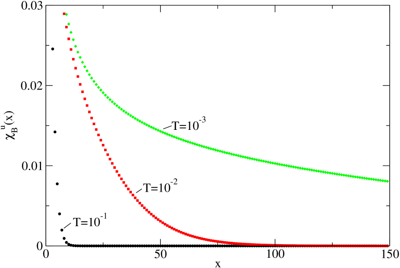
Figure 2: The uniform part of the local boundary susceptibility $\chi_{B}^{u}(x)$ following from Eq. (4.4) for $K=1.2$ at different temperatures. The boundary susceptibility $\chi_{B}$ is obtained by integrating over $\chi_{B}^{u}(x)$ leading to a $1/T^{3-2K}$ divergence if $K<3/2$.

At zero temperature with a finite magnetic field, a similar singular behaviour appears in the field dependence of the boundary spin susceptibility given by,

$$\chi_{\rm B}(T=0)=\lambda\left(\frac{K}{v}\right)^{2}\sin(\pi K)\Gamma(3-2K)\left(\frac{Kh}{v}\right)^{2K-3}.$$ (4.8)

The zero temperature susceptibility can also be derived from the Bethe ansatz exact solution by using the Wiener-Hopf method. This has been done in Ref. [24, 25] and agrees with the expression above.

5 The isotropic case $\Delta=1$

At the isotropic point Umklapp scattering becomes marginal. Instead of using (2.14) one can write the marginal perturbation in a manifestly SU(2) invariant form using the SU(2) current operators. The perturbation in this formulation becomes

$$\delta H=\int\frac{dx}{2\pi}[g_{\parallel}J_{z}\bar{J}_{z}+\frac{g_{\perp}}{2}(J_{+}\bar{J}_{-}+J_{-}\bar{J}_{+})].$$ (5.1)

The small running coupling constants $g_{\parallel}$, $g_{\perp}$ fulfil a set of known Renormalisation Group (RG) equations [4, 3] and are in general functions of the different scales, $T,L$ and $h$, involved. The perturbation (5.1) can be split into two parts: $J_{z}\bar{J}_{z}\propto\Pi^{2}-(\partial_{x}\phi)^{2}$ and $J_{+}\bar{J}_{-}+J_{-}\bar{J}_{+}\propto\cos(\sqrt{8\pi}\phi)$. The first term can be absorbed in the free electron Hamiltonian (2.2) by a rescaling of the fields $\Pi$ and $\phi$. This leads to a renormalisation of the Luttinger parameter $K\to 1+g_{\parallel}/2+\mathcal{O}(g^{2})$ (see B for details). With this replacement in (2.9) we see that the susceptibility at the isotropic point in the thermodynamic limit is now given by

$$\chi_{\mbox{\tiny bulk}}(T)=\frac{1}{\pi^{2}}\left(1+\frac{g(T)}{2}+\mathcal{O}(g^{2})\right)\;,$$ (5.2)

a result first derived in Ref. [6]. The second term leads in lowest order to a replacement $\lambda\to-g_{\perp}/4$. More generally, the results for the anisotropic model derived in the previous sections have to be expanded in powers of $1-1/K$ and then re-expressed in terms of the coupling constants $g_{\parallel}$ and $g_{\perp}$ [4]. For details the reader is referred again to B. Here we only want to give the main results.

First, we consider the isotropic limit of our first order result for the boundary susceptibility (4.6). This leads to

$$\chi_{B}^{(1)}=-\frac{g_{\perp}}{12T}-\frac{g_{\parallel}g_{\perp}}{8T}\left(\frac{1}{2}-\frac{\Psi^{\prime\prime}(1)}{\pi^{2}}\right)\,.$$ (5.3)

The second order result derived in A also yields a contribution in quadratic order in $g$

$$\chi_{B}^{(2)}\approx\frac{g_{\perp}^{2}}{8T}\cdot 0.11\;.$$ (5.4)

Here the factor $0.11$ stems from a numerical evaluation of the integral in (A) for $K=1$. With $g_{\parallel}\to g$, $g_{\perp}\to-g$ we therefore obtain up to quadratic order in $g$

$$\chi_{B}=\frac{a}{\pi^{2}}+\frac{g}{12T}+\frac{g^{2}}{8T}\left(0.66-\frac{\Psi^{\prime\prime}(1)}{\pi^{2}}\right)+\mathcal{O}(g^{3})\,.$$ (5.5)

Here $g=g(T)$ and is given by [4]

$$1/g+\ln(g)/2=\ln\left(T_{0}/T\right)\;,$$ (5.6)

with $T_{0}=\sqrt{\pi/2}e^{1/4+\gamma}$ where $\gamma$ is the Euler constant. Note, that the scale in the logarithm, $T_{0}$, is chosen according to the expansion of the bulk susceptibility. $T_{0}$ is non-universal and can be fixed differently to achieve the best possible agreement with the expansion of the boundary susceptibility at the isotropic point. However, this is not important for $\chi_{B}$ as it only influences sub-leading terms so we keep the scale as set by the bulk part in order to have a single $g$ in the formula for $\chi(L,T)$ discussed in the following. A more detailed discussion of this point is presented in B.

In addition, we have added a contribution $\sim Ka/(2\pi v)$ to (5.5) with some constant $a$ stemming from the boundary operator as in the anisotropic case. However, the constant (3.20) obtained by Bethe Ansatz in the anisotropic case does have an accumulation point of singularities at $K=1$ making it impossible to extract the value at the isotropic point from this formula. If one considers, on the other hand, the integral for the boundary susceptibility derived directly by Bethe Ansatz for the isotropic case (see Eq. (36) in [24]), this task is difficult as well because the logarithmic contributions coming from the cut along the imaginary axis completely dominate. Indeed, at low-temperatures the constant contribution is less important than any of the logarithmic terms coming from the expansion of $\chi_{B}$ outlined above. Nevertheless, this constant becomes important again at higher temperatures (but still $T/J\ll 1$) as in the anisotropic case. We will therefore use it as a fitting parameter when comparing to the numerical data in Fig. 3.

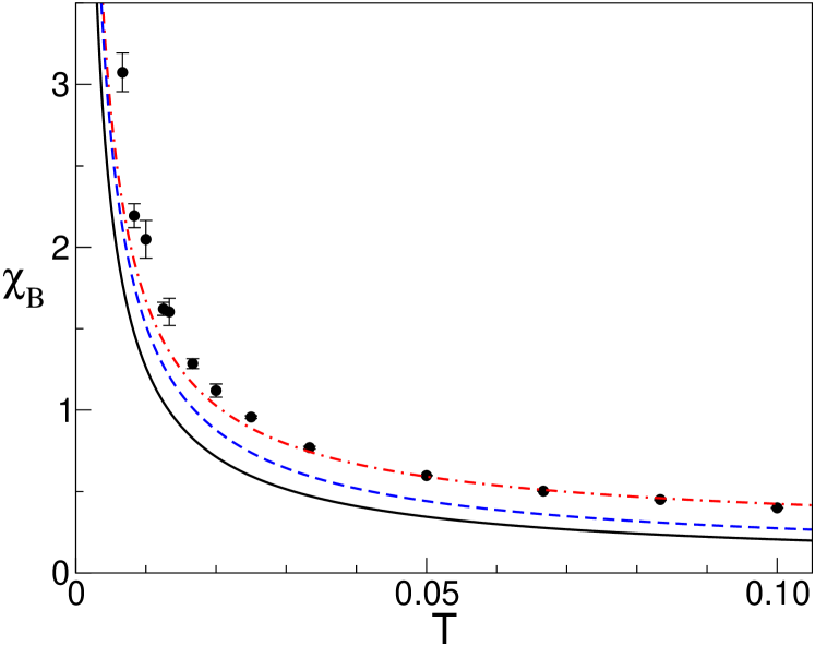
Figure 3: Comparison between QMC results (dots) and the field theory result (5.5). The black solid line corresponds to taking into account the first order in $g$ term only, the blue dashed line is the result with the second order term included, and the red dot-dashed line is obtained by adding a constant $Ka/2\pi v$ with $a=1.5$ ($K=1$, $v=\pi/2$). The QMC data for $\chi_{B}$ have been obtained by subtracting the bulk susceptibility known from Bethe ansatz [6] from numerical data for $\chi(L)$. The chain length $L$ has always been chosen such that $TL/v\gtrsim 4$. In addition, the susceptibility has been calculated for lengths $L$ and $L+1$ and then averaged to further reduce finite size effects (see also Eq. (5.8) and Fig. 4 below).

Note, that $a$ now effectively also partly incorporates higher order logarithmic corrections to (5.5) as well as the constant coming from the boundary operator. Furthermore, we must in principle replace $Ka/(2\pi v)\to(a/\pi^{2})(1+g/2+g^{2}/4+\cdots)$ (see B). However, because the logs dominate at low temperatures this merely leads to a small rescaling of $a$ which we will ignore because $a$ is an “effective constant” in any case. Solving Eq. (5.6) we can also write the boundary susceptibility as

$$\chi_{B}=\frac{1}{12T\ln(T_{0}/T)}\left(1-\frac{\ln\ln(T_{0}/T)}{2\ln(T_{0}/T)}+\cdots\right)\;.$$ (5.7)

This means that even in the limit $T/v\gg 1/L$ we find a Curie-like contribution albeit with a “Curie constant” which depends logarithmically on temperature.

If $T/v$ becomes of order $1/L$ the susceptibility can no longer be split into a bulk and a boundary contribution. However, we can still subtract the known bulk contribution and define a quantity $\delta\chi_{FS}$ as in Eq. (1.1). In a first approximation, we can use the thermodynamic limit result for $\chi_{B}$, Eq. (5.5), and add the leading finite size corrections stemming from the scaling part (second term in the last line of Eq. (2.13)). This leads to

$$\delta\chi_{FS}(L,T)\approx\chi_{B}(T)\pm\frac{8L^{2}T}{\pi^{2}}(1+g)\exp[-2LT(1+g/2)]$$ (5.8)

where the plus (minus) sign refers to chains of odd (even) length and we have replaced $K\to 1+g/2$ with $g$ determined by Eq. (5.6). A comparison between this formula and QMC data is shown in Fig. 4.

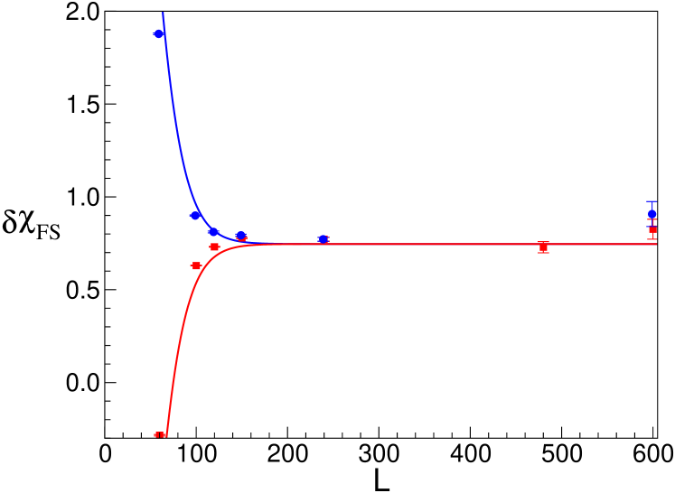
Figure 4: QMC data for the susceptibility $\delta\chi_{FS}$ at temperature $T=J/30$ as a function of chain length. These data have been obtained by subtracting the bulk susceptibility known from Bethe ansatz [6] from numerical data for $\chi(L)$. The red squares (blue circles) correspond to even (odd) chain length, respectively. The lines represent the approximation (5.8).

Note, that Eq. (5.8) implies an almost perfect cancelation of finite size corrections when calculating the susceptibility for lengths $L$ and $L+1$ and then taking the average. This property has been used to improve the numerical data for $\chi_{B}$ presented in Fig. 3.

To obtain the result for $\chi(L,T)$ at the isotropic point in general, we have to consider both parts of the perturbation (5.1): First, we have to replace $K\to 1+g/2$ in the exponentials of (2.9). For the correction (3.12) we can only obtain a result to first order in $g$ because we do not know the analytical solution of the integral and therefore cannot easily expand it around $K=1$. The result to first order in $g$ is readily obtained by just replacing $\lambda\to g/4$ and evaluating the integral for $K=1$. Now, however, the running coupling constant $g$ depends on two scales: the length $L$ and temperature $T$. There is no general solution of the renormalisation group equations if two different scales are involved. At low enough energies, however, the smaller length scale will always dominate and the running coupling constant becomes [4]

$$1/g+\ln(g)/2=\ln\left(\sqrt{2/\pi}e^{1/4+\gamma}\mbox{min}[L,v/T]\right)\;.$$ (5.9)

In addition, the constant $a$ stemming from the boundary operator is still present and we will use it again as a fitting parameter. Note, that $a$ now will be different from the one obtained by fitting the numerical data for $\chi_{B}$ as it also partly incorporates the logarithmic terms now taken into account only to lowest order.

To summarise, the susceptibility for the isotropic case is given by $\chi(L,T)=\chi_{0}+\delta\chi_{1}$ with the replacements $K\to 1+g(L,T)/2+a/L$ in the exponentials of (2.9) and $\lambda\to g(L,T)/4$ in (3.12). A comparison between this formula and QMC data for chains of different lengths is shown in Fig. 5.

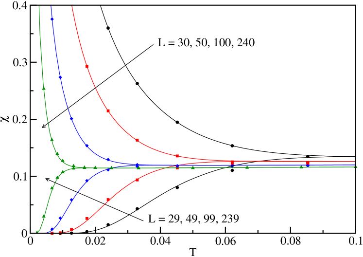
Figure 5: Comparison for $\Delta=1$ between QMC results (symbols) and the field theory result (lines) with $a=4$ for chains of different length $L$.

Here we find that $a\approx 4$ works best describing the numerical data over a wide temperature range and for different even and odd chain lengths very accurately.

The disadvantage of this formula for $\chi(L,T)$ is, that the integral in (3.12) has to be evaluated numerically for each length and temperature considered. In the next section we will derive a much simpler formula in the limit $T/J\ll 1/L$. We find empirically that this formula describes the susceptibility over a much larger range of temperatures than anticipated making it useful to fit experimental data without the necessity to evaluate the integral in (3.12) and without having a free fit parameter.

6 The ground state limit: $LT/v\to 0$

Next, we want to consider the limit $LT/v\to 0$. We have already shown in Eq. (2.13) that the scaling part of the susceptibility shows a Curie-like divergence if the chain length is odd and an exponentially suppressed behaviour if it is even. For the first order correction (3.12) we will concentrate again on the case $K<3/2$ where the cutoff can be dropped. In the limit $LT/v\to 0$ we find $\eta\left(\mbox{e}^{-\frac{\pi v}{TL}}\right)\to\mbox{e}^{-\frac{\pi v}{24TL}}$, $\theta_{1}\left(\pi y,\mbox{e}^{-\frac{\pi v}{2TL}}\right)\to 2\mbox{e}^{-\frac{\pi v}{8TL}}\sin(\pi y)$ and

$$g_{0}\left(y,\mbox{e}^{-\frac{\pi v}{KTL}}\right)\to\left\{\begin{array}[]{cc}0&\mbox{L odd}\\[8.5359pt] -2\cos(4\pi y)\mbox{e}^{-\frac{\pi v}{KTL}}+2\mbox{e}^{-\frac{\pi v}{KTL}}&\mbox{L even}\end{array}\right.$$ (6.1)

Here we have expanded $g_{0}$ only to first power in the small parameter $\mbox{e}^{-\frac{\pi v}{KTL}}$. For $L$ odd the first non-vanishing contribution is second order. As the scaling part shows a power-law divergence in this case, any exponentially small corrections can be safely neglected in any case. For $L$ even, on the other hand, they are important as the scaling part is also exponentially small. In the even case we can now evaluate the integral and find

$$\delta\chi_{1}(LT/v\to 0)=\left\{\begin{array}[]{cc}0&\mbox{L odd}\\[8.5359pt] \frac{2\lambda}{T^{2}}\left(\frac{\pi}{L}\right)^{2K}\frac{\Gamma(3-2K)}{\Gamma(2-K)\Gamma(3-K)}\mbox{e}^{-\frac{\pi v}{KTL}}&\mbox{L even}\end{array}\right.$$ (6.2)

Finally, lets consider the contribution $\delta\chi_{2}$. For $L$ odd $g_{2}(\mbox{e}^{-\frac{\pi v}{KLT}})\to 0$ in lowest order whereas $g_{2}(\mbox{e}^{-\frac{\pi v}{KLT}})\to 2\mbox{e}^{-\frac{\pi v}{KLT}}$ for $L$ even. This leads to

$$\delta\chi_{2}=\left\{\begin{array}[]{cc}0&\mbox{L odd}\\[8.5359pt] \frac{2\pi v}{KT^{2}L^{3}}\mbox{e}^{-\frac{\pi v}{KTL}}\cdot a&\mbox{L even}\end{array}\right.$$ (6.3)

For the susceptibility in the limit $LT/v\to 0$ we therefore find

$$\chi(LT\to 0)=\left\{\begin{array}[]{cc}\frac{1}{4LT}&\mbox{L odd}\\[8.5359pt] \frac{2}{LT}\mbox{e}^{-\frac{\pi v}{KTL}}\left[1+\lambda\frac{\beta\pi^{2K}}{L^{2K-1}T}+\frac{\pi v}{KL^{2}T}a\right]&\mbox{L even}\end{array}\right.$$ (6.4)

where $\beta=\Gamma(3-2K)/[\Gamma(2-K)\Gamma(3-K)]$. So corrections to the scaling limit result in first order in $\mbox{e}^{-\frac{\pi v}{TL}}$ are only present in the case of even chain length. However, even in this case these corrections are suppressed by additional powers of $1/(LT)$. So one might think that Eq. (6.4) is of purely academic interest. However, as we will show below, it enables us to derive a simple formula for the susceptibility of the isotropic chain which works over a much larger range of temperatures and lengths than anticipated.

In the isotropic case we have to replace $K\to 1+g_{\parallel}(L)/2$ in the scaling part (2.9). Furthermore $\lambda\to-g_{\perp}(L)/4$, so that (6.4) at the isotropic point reads

$$\chi(LT\to 0)=\left\{\begin{array}[]{cc}\frac{1}{4LT}&\mbox{L odd}\\[8.5359pt] \frac{2}{LT}\mbox{e}^{-\frac{\pi^{2}}{2TL}}\left[1+\frac{\pi^{2}}{4LT}g_{\parallel}(L)-\frac{\pi^{2}}{4LT}g_{\perp}(L)+\frac{\pi^{2}}{2L^{2}T}a\right]&\mbox{L even}\end{array}\right.$$ (6.5)

where $v=\pi/2$ has been employed. Note that with $g_{\parallel}\to g$, $g_{\perp}\to-g$ the replacement $K\to 1+g_{\parallel}(L)/2$ in the scaling part and the first order contribution in $\lambda\to-g_{\perp}(L)/4$ both produce exactly the same correction $\frac{\pi^{2}}{4LT}g(L)$ in the brackets in (6.5). Here $g(L)$ is given by (5.6) with $L$ being the relevant scale in this limit. We want to stress that both terms yielding exactly the same contribution in the limit considered here contribute very differently in the thermodynamic limit. Whereas the $g_{\parallel}$-part leads to a correction to the bulk susceptibility, the $g_{\perp}$-part determines the boundary susceptibility.

Ignoring the contribution $\sim a$ which comes from the boundary operator and is suppressed by an additional power of $L$ we can therefore obtain exactly the same expansion by replacing $1/K\to 1-g(L)$ in the exponentials of (2.9). I.e., we can absorb the first order correction $\delta\chi_{1}$ into the scaling form. This leads to the formula

$$\chi=\frac{1}{LT}\frac{\sum_{S_{z}}S_{z}^{2}\exp\left[-\frac{\pi^{2}}{2LT}(1-g(L))S_{z}^{2}\right]}{\sum_{S_{z}}\exp\left[-\frac{\pi^{2}}{2LT}(1-g(L))S_{z}^{2}\right]}\,.$$ (6.6)

This formula should be valid in the limit $LT/v\to 0$ when only the ground state and the lowest excited states contribute to the sum over $S_{z}$. One easily verifies that Eq. (6.5) is indeed reproduced in this limit: For $L$ odd we take only the states $S_{z}=\pm 1/2$ into account and the correction $1-g(L)$ cancels out. For $L$ even we consider the ground state $S_{z}=0$ and the first excited state $S_{z}=\pm 1$. Expanding in $g(L)$ then leads to (6.5).

So starting from our general result for the susceptibility of finite open chains we have found that the correction to the excitation energy of the lowest excited states with $S_{z}\pm 1$ in the isotropic case is given by $E\to(\pi v/L)[1-g(L)]$. This agrees with the findings in Ref. [14]. Corrections to higher excited states are not of such simple form, and, in general, it is therefore not possible to absorb these corrections into the scaling part.

Empirically, however, we find that (6.6) works quite well over a much larger range of lengths and temperatures than one might anticipate. In Fig. 6 we compare this formula again to QMC data.

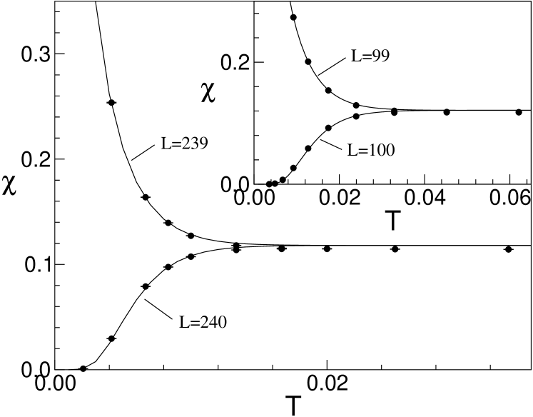
Figure 6: Comparison for $\Delta=1$ between QMC results (dots) and the field theory result (6.6) in the limit $LT/v\to 0$ (lines).

Although the agreement at higher temperatures where the susceptibility becomes constant is not perfect, the errors in this region are only about $3\%$.

7 The averaged susceptibility and the effective Curie constant

In this section we want to discuss the averaged susceptibility of the isotropic Heisenberg chain for a concentration of chain breaks $p$ as defined in Eq. (1.2). Here we have assumed that we have a completely random (Poisson) distribution of impurities. However, we could obtain $\chi_{p}$ for any other distribution as well. $\chi_{p}$ can be calculated by using our field-theory results in section 5 for $L\gtrsim 10$ and $T/J\lesssim 0.1$ in combination with exact diagonalisation or QMC results for shorter chains. This method has been used in Ref. [26] to analyse susceptibility data for Sr₂Cu_1-xPd_xO_3+δ [29]. Based on our analysis of the limits $LT/v\to 0$ and $LT/v\to\infty$ in the previous sections we want to derive here a simple formula which allows to determine the concentration of chain breaks by fitting the measured susceptibility.

We have seen that there are no corrections to the scaling limit result in the limit $LT/v\to 0$ for odd chains. For even chains the susceptibility is exponentially small in this limit in any case so that even chain segments practically do not contribute to the average in (1.2). In the opposite limit we can write $\chi(L)=L\chi_{\mbox{\tiny bulk}}+\chi_{B}$. We now assume that the crossover occurs at some length $L_{c}=\gamma J/T$ where $\gamma$ is a crossover parameter which we expect to be of order one. For the average susceptibility we can therefore write

$$\chi_{p} \approx \frac{p^{2}}{4T}\sum_{L\;\mbox{\tiny odd}}^{L_{c}}(1-p)^{L}+p^{2}\sum_{L_{c}}^{\infty}(L\chi_{\mbox{\tiny bulk}}+\chi_{B})(1-p)^{L}$$

$$= \frac{p}{4T}\frac{1-p}{2-p}\left(1-(1-p)^{\gamma/T}\right)+(1-p)^{\gamma/T}\left[\left(1-p+\frac{p\gamma}{T}\right)\chi_{\mbox{\tiny bulk}}+p\chi_{B}\right]$$

and we use the field theory result for the bulk susceptibility [4]

$$\chi_{\mbox{\tiny bulk}}=\frac{1}{\pi^{2}}\left(1+\frac{g(T)}{2}+\frac{3g^{3}(T)}{32}+\sqrt{3}{\pi}T^{2}\right)$$ (7.2)

where the $T^{2}$-term stems from the irrelevant operators with scaling dimension $4$. The boundary susceptibility $\chi_{B}$ is given by (5.5) with $a=1.5$ as in Fig. 3.

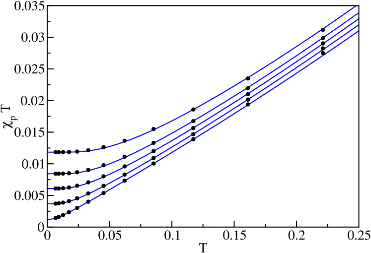
Figure 7: $T\chi_{p}$ for $p=0.01,0.03,0.05,0.07,0.1$ from bottom to top. The black dots are obtained by using QMC data for $\chi(L)$ and the lines represent the fitting formula (7) with $\gamma=1$.

A comparison between QMC data for $\chi_{p}$ and (7) with $\gamma=1$ for various impurity concentrations is shown in Fig. 7.

The impurity part and an effective Curie constant $C$ can then be defined according to Eq. (1.2) by

$$p\delta\bar{\chi}_{FS}=\chi_{p}-(1-p)\chi_{\mbox{\tiny bulk}}=p\frac{C}{T}\;.$$ (7.3)

This effective Curie constant is shown in Fig. 8.

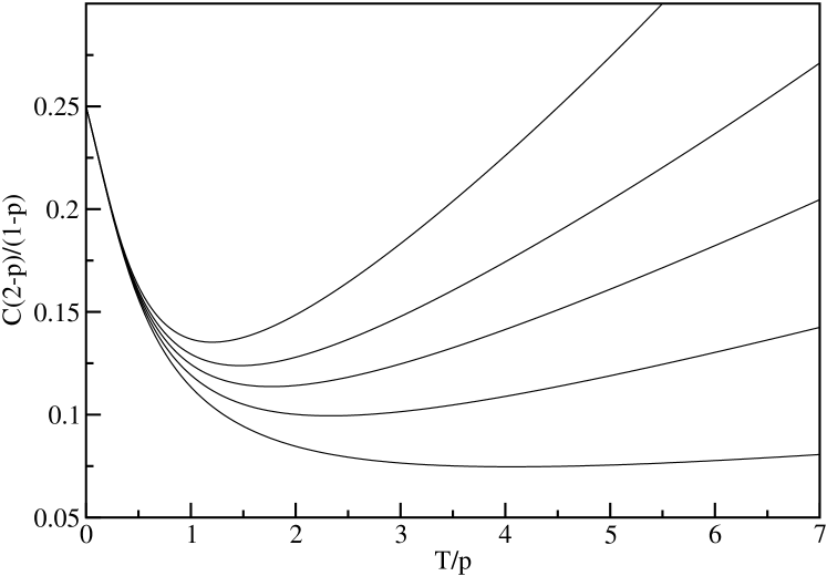
Figure 8: The effective Curie constant as defined in Eq. (7.3) for $p=0.01,0.03,0.05,0.07,0.1$ (from bottom to top) as a function of $T/p$.

Note, that only in the extreme low-temperature limit the usual Curie constant $C\to 1/4\cdot(1-p)/(2-p)\approx 1/8$ (half of the chains contribute a Curie constant of $1/4$ for $p\ll 1$) is recovered. However, $C(2-p)/(1-p)$ as a function of $T/p$ shows an almost perfect collapse (scaling) for different impurity concentrations if $T/p\lesssim 1/2$. At higher temperatures this scaling no longer holds because the boundary contribution $\chi_{B}$ is not a scaling function in $T/p$. The non-trivial temperature dependence of the effective Curie constant, in particular the finite temperature minimum, and the scaling at temperatures $T\lesssim p/2$ provide a way to test this scenario experimentally.

8 Inter- and Intrachain couplings

In any real system there are residual couplings between the chain segments in the principal chain direction (intrachain couplings). In addition, there are also perpendicular couplings between the chains (interchain couplings) which at low enough temperatures will destroy the one dimensionality of the system and usually induce some sort of magnetic order. In Sr₂CuO₃, for example, the nearest-neighbour Heisenberg coupling along the chain direction (b-axis) is estimated to be $J\sim 2200$ K whereas the couplings along the other axis are orders of magnitude smaller ($J_{a}\sim 5$ K, $J_{c}\sim 10^{-3}$ K) [28]. Furthermore, it has been pointed out that the next-nearest-neighbour coupling along the chain direction is probably not that small, $J_{2}\sim 140$ K [35]. This irrelevant coupling will only cause small corrections to the susceptibility of an isolated chain segment by changing the marginally irrelevant coupling constant $\lambda$. However, it induces a coupling between different chain segments even when the nearest-neighbour exchange $J$ is absent due to a non-magnetic impurity. Note, that there is no frustration in this case and $J_{2}$ just acts as an effective coupling $J^{\prime}$ between the chain ends as shown in Fig. 9.

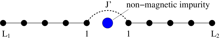
Figure 9: Two chain segments with length $L_{1}$ and $L_{2}$, respectively, coupled by a weak intrachain coupling $J^{\prime}\ll J$.

Although the next-nearest neighbour coupling across an impurity can differ from the one across a magnetic ion, we will assume that it is still of the same order of magnitude, i.e., $J^{\prime}\sim J_{2}$.

The susceptibility of the weakly coupled chains is given by

$$\chi=\frac{1}{LT}\left\langle\left(\sum_{i=1}^{L_{1}}S_{1i}^{z}+\sum_{j=1}^{L_{2}}S_{2j}^{z}\right)^{2}\right\rangle$$ (8.1)

with $L=L_{1}+L_{2}$. Here $S_{1i}^{z}$ ($S_{2j}^{z}$) denotes the $z$-component of the spin on chain 1 (2) at site $i$ ($j$), respectively. For $J^{\prime}\ll J$ we can treat this coupling using perturbation theory. In zeroth order this lead to $\chi^{(0)}=(L_{1}\chi_{1}^{(0)}+L_{2}\chi_{2}^{(0)})/L$. In first order only the longitudinal part of the coupling contributes and we obtain

$$\delta\chi = -\frac{2J^{\prime}}{LT^{2}}\left\langle\sum_{i=1}^{L_{1}}S^{z}_{1i}S^{z}_{11}\right\rangle\left\langle\sum_{j=1}^{L_{2}}S^{z}_{2j}S^{z}_{21}\right\rangle$$ (8.2)

$$= -\frac{2J^{\prime}}{LT^{2}}\left\langle S^{z}_{1\mbox{\tiny tot}}S^{z}_{11}\right\rangle\left\langle S^{z}_{2\mbox{\tiny tot}}S^{z}_{21}\right\rangle=-\frac{2J^{\prime}}{L}\chi_{11}\chi_{21}$$

where $\chi_{l1}=\partial<S^{z}_{l1}>/(\partial h)$ is the susceptibility of the boundary spin $S^{z}_{l1}$ and $S^{z}_{l\mbox{\tiny tot}}=\sum_{i=1}^{L_{l}}S^{z}_{li}$ ($l=1,2$), respectively. The extra factor of 1/T arises due to time-translational invariance and the imaginary time integral in the first order perturbation theory formula. Because of the broken spatial-translational invariance, the local susceptibility is position dependent and the boundary spins are more susceptible than the spins deep inside the chain. These effects have been studied in detail in Refs. [18, 24]. As we are here just interested in an order of magnitude estimate of the effect of intrachain coupling on $\chi_{p}$ we can replace the susceptibility of the boundary spin $\chi_{l1}$ by the average susceptibility per site $\chi_{l}^{(0)}$. This leads to $\delta\chi\approx-2(J^{\prime}/L)\chi_{1}^{(0)}\chi_{2}^{(0)}$. Assuming further that for an impurity concentration $p$ all chain segments have length $L\sim 1/p$ we find

$$\delta\chi_{p}\sim J^{\prime}p\chi_{p}^{2}\;.$$ (8.3)

At $T\ll pv$ we have $\chi_{p}\sim p/(8T)$. The correction (8.3) therefore becomes of order $\chi_{p}$ at $T\sim J^{\prime}p^{2}$. For temperatures $T\gg J^{\prime}p^{2}$ intrachain coupling can therefore be neglected.

Although first order perturbation theory can give us the temperature scale where intrachain coupling becomes important, it is not sufficient once this scale is approached. This can be seen by a scaling analysis. We have $S^{z}\sim\partial_{x}\phi$ with scaling dimension one. In $n$-th order perturbation theory in the intrachain coupling $J^{\prime}$, the longitudinal part of the coupling therefore yields $\chi^{(n)}\sim(TL)^{-1}(J^{\prime}/TL^{2})^{n}$. We can therefore write the susceptibility in scaling form

$$\chi \sim \frac{1}{LT}\left(1+\frac{J^{\prime}}{L^{2}T}+\frac{J^{\prime 2}}{L^{4}T^{2}}+\frac{J^{\prime 3}}{L^{6}T^{3}}+\cdots\right)\;.$$ (8.4)

Replacing again $L\sim 1/p$ we find for the averaged susceptibility

$$\chi_{p} \sim \frac{p}{T}\left(1+\frac{J^{\prime}p^{2}}{T}+\left(\frac{J^{\prime}p^{2}}{T}\right)^{2}+\left(\frac{J^{\prime}p^{2}}{T}\right)^{3}+\cdots\right)\;.$$ (8.5)

This means that at temperatures where intrachain coupling $J^{\prime}$ can no longer be neglected, $T\sim J^{\prime}p^{2}$, perturbation theory in $J^{\prime}$ breaks down. At temperatures $T\ll J^{\prime}p^{2}<Jp$, on the other hand, we can obtain an effective model by replacing all segments of odd length by $S=1/2$ spins. The couplings between these effective $S=1/2$ will then be random with a very broad distribution. According to Fisher [36] we might therefore expect that a system of weakly coupled chain segments renormalises at very low temperatures to the infinite random fixed point. In any realistic system, however, there will be also interchain couplings between the chain segments preventing the system from reaching this fixed point.

An interchain coupling between two chain segments is shown in Fig. 10.

Figure 10: Two chain segments with length $L_{1}$ and $L_{2}$, respectively, have an overlap of $n$ sites and are coupled by an interchain coupling $\tilde{J}$.

In first order perturbation theory we obtain in this case

$$\delta\chi^{(1)} = -\frac{2\tilde{J}}{LT^{2}}\sum_{k=1}^{n}\left\langle\sum_{i=1}^{L_{1}}S^{z}_{1,i}S^{z}_{1,k}\right\rangle\left\langle\sum_{j=1}^{L_{2}}S^{z}_{2,j}S^{z}_{2,n+1-k}\right\rangle$$

$$= -\frac{2\tilde{J}}{LT^{2}}\sum_{k=1}^{n}\left\langle S^{z}_{1\mbox{\tiny tot}}S^{z}_{1,k}\right\rangle\left\langle S^{z}_{2\mbox{\tiny tot}}S^{z}_{2,n+1-k}\right\rangle=-\frac{2\tilde{J}}{L}\sum_{k=1}^{n}\chi_{1,k}\chi_{2,n+1-k}$$

where $\chi_{l,k}$ denotes the local susceptibility of the $l$-th chain at site $k$. To simplify matters, we consider the case of two chains with equal lengths $L_{1}=L_{2}=L$ which completely overlap, i.e., $n=L$. In this case Eq. (8) becomes

$$\delta\chi^{(1)}=-\frac{2\tilde{J}}{L}\sum_{k=1}^{L}\chi_{1,k}\chi_{2,k}\>.$$ (8.7)

At $T\ll pv$ we can again set $\chi_{1,k}\sim\chi_{p}\sim p/T$ which leads to $\delta\chi^{(1)}_{p}\sim\tilde{J}p^{2}/T^{2}$. This becomes of order $\chi_{p}$ at temperatures $T\sim\tilde{J}p$. As $\tilde{J}$ is of order of the Néel temperature $T_{N}$ this scale is completely irrelevant. However, for a system with open boundaries the local susceptibility has also a staggered part [18, 12] which will contribute to (8.7). This is a consequence of the $S^{z}$-operator having a staggered part, $S^{z}_{k,st.}\sim c(-1)^{k}\cos\sqrt{2\pi}\phi$, where $c$ is a constant. For a chain with odd length in the ground state limit, $T\ll 1/L$, we find [12]

$$\chi_{k}^{st.} = \frac{1}{T}\langle S^{z}_{tot}S^{z}_{k,st.}\rangle\approx\frac{1}{T}\sum_{\pm}\langle\pm|S^{z}_{tot}S^{z}_{k,st.}|\pm\rangle\approx(-1)^{k}\frac{c}{T}\sqrt{\frac{\pi}{2L}\sin\frac{\pi k}{L}}$$ (8.8)

where $|\pm\rangle$ is the ground state with $S^{z}_{tot}=\pm 1/2$, respectively. This leads to $\delta\chi^{(1)}\sim\tilde{J}/(LT^{2})\sim\tilde{J}p/T^{2}$ and therefore dominates compared to the contribution originating from the uniform part of the local susceptibility. It becomes of order $\chi_{p}$ at temperatures $T\sim\tilde{J}$.

Finally, we want to consider the “clean limit”, $T\gg pv$. In this case, the Néel temperature $T_{N}$ can be determined by treating the interchain coupling in mean field theory. This leads to the well known condition

$$z\tilde{J}\chi_{st}(T_{N})=1$$ (8.9)

where $\chi_{st}$ is the staggered susceptibility, i.e., the staggered response to the effective staggered field originating from the other chains and $z$ is the coordination number. Because $\chi_{st}(T)\sim 1/T$ we obtain that $T_{N}\sim\tilde{J}$. The same condition for the breakdown of one-dimensionality in this limit is obtained by considering the contribution of the staggered part of the $S^{z}$-operator to the susceptibility in second order perturbation theory in the interchain coupling.

We therefore conclude that our results for the averaged susceptibility $\chi_{p}$ in the previous sections are applicable as long as $T\gg\mbox{Min}(\tilde{J},p^{2}J^{\prime})$.

9 Experimental situation

The best known realisation of the spin-$1/2$ Heisenberg chain is Sr₂CuO₃. Here copper is in a 3d⁹ configuration and has spin $1/2$. The Heisenberg couplings between these spins are spatially very anisotropic as already mentioned in the previous section. For $T\gg J_{a}\sim 5$ K interchain coupling can therefore be neglected and the magnetic properties are described by the one-dimensional isotropic Heisenberg model.

The doped compound Sr₂Cu_1-xPd_xO₃ has been studied by Kojima et al [29]. Here palladium has spin zero and therefore serves as a non-magnetic impurity. Impurity concentrations from $x=0.5\%$ up to $x=3\%$ have been studied. This means that $x^{2}J_{2}$ with $J_{2}\sim 140$ K is small even compared to $J_{a}$. In this material the limit where our theory is applicable is therefore set by the interchain coupling, $T\gg J_{a}\approx 5$ K.

The theoretical analysis of the susceptibility measurements on Sr₂Cu_1-xPd_xO₃ is hampered by the fact that even the pure system Sr₂CuO₃ already shows Curie-like contributions at low temperatures [27, 28]. It has been observed that these contributions can be significantly reduced by annealing and two explanations have been offered: Excess oxygen might be present in the as grown compound. Most likely, each excess oxygen would then dope two holes into the chain leading to two Zhang-Rice singlet type states as in the high-$T_{c}$ compounds. Assuming that these holes are relatively immobile, they effectively act as chain breaks. In this scenario the Curie-type contribution in the “pure compound” is caused by the mechanism described in this paper. Indeed, it has been shown [26] that the susceptibility data for the as grown crystal sample in [28] can be well described by assuming a concentration of chain breaks, $p=0.6\%$. For the powder samples studied by Ami et al. [27] an alternative explanation was proposed by Hill et al. based on the observation that Sr₂CuO₃ decomposes into Sr₂Cu(OH)₆ under exposure to air and water [37]. The copper spins-$1/2$ in Sr₂Cu(OH)₆ are only weakly coupled according to Hill et al. and can therefore induce a true Curie contribution as opposed to the more complicated behaviour expected in the chain break scenario. It is, however, hard to see how this could also explain the Curie-like contributions observed on single crystals by Motoyama et al. [28]. We therefore believe that the excess oxygen scenario is the most plausible explanation in this case.

The Sr₂Cu_1-xPd_xO₃ samples investigated by Kojima et al. have not been annealed so that we expect chain breaks due to excess oxygen in addition to the once caused by palladium. Furthermore, it can certainly not be excluded that there are indeed additional true paramagnetic impurity contributions caused by decomposition or other mechanisms. This makes a thorough theoretical analysis very difficult. In [26] such an analysis has been performed under the assumptions that true paramagnetic Curie contributions can be neglected and that excess oxygen will lead to immobile holes acting as additional chain breaks. The measured susceptibility $\chi^{\mbox{\tiny exp.}}$ then consists of a temperature independent part $\chi^{\prime}$ due to core diamagnetism and Van Vleck paramagnetism and $\chi_{p}$ coming from the Heisenberg chains with impurity concentration $p$. Here $p=x+\delta$ has to be considered as a fitting parameter consisting of the nominal palladium concentration $x$ and the concentration of additional chain breaks $\delta$ due to excess oxygen. A best fit of the experimental data was obtained in [26] with the two parameters $p$, $\chi^{\prime}$ as displayed in Table 1.

Table 1: Concentration $x$ of Pd ions in experiment compared to impurity concentration $p$ and constant contribution $\chi^{\prime}$ yielding the best theoretical fit. The first line corresponds to the “as grown” sample of Sr₂CuO₃ from Ref. [28].

$x$ (Exp.)	$p$ (Theory)	$\chi^{\prime}$ [emu/mol]
$0.0$	$0.006$	$-7.42\times 10^{-5}$
$0.005$	$0.012$	$-7.7\times 10^{-5}$
$0.01$	$0.014$	$-7.5\times 10^{-5}$
$0.03$	$0.024$	$-7.5\times 10^{-5}$

For the sample with a nominal Pd concentration of $3\%$ our best fields has yielded $p=2.4\%$, i.e., less than the nominal concentration. One might speculate that the Pd ions cluster or that part go in at interstitial positions instead of replacing Cu ions thus reducing the number of chain breaks created.

Here we want to go one step further and compare the effective Curie constant extracted from the experimental data

$$C^{\mbox{\tiny exp.}}=\frac{T}{p}\left[\chi^{\mbox{\tiny exp.}}-\chi^{\prime}-(1-p)\chi_{{\mbox{\tiny bulk}}}\right]$$ (9.1)

with the theoretical prediction. We will use the same values for the concentration of chain breaks $p$ and the constant contribution to the susceptibility $\chi^{\prime}$ as in Table 1. For $\chi_{\mbox{\tiny bulk}}$ we employ the field theoretical result (7.2). The result is shown in Fig. 11.

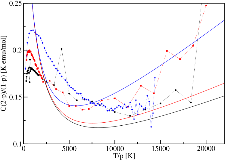
Figure 11: The effective Curie constant (9.1) extracted from susceptibility data for Sr₂Cu_1-xPd_xO₃ [29]. The nominal Pd concentration is $x=0.5\%$ (black circles), $x=1\%$ (red squares), and $x=3\%$ (blue diamonds). The solid lines denote the theoretical result (7.3) for $p=1.2\%$, $p=1.4\%$, and $p=2.4\%$ (from bottom to top).

Although the agreement is far from perfect we see that the Curie constant extracted from experiment does indeed show a non-trivial temperature dependence. In particular, there is a finite temperature minimum although at higher temperatures than predicted theoretically. The maximum at low temperatures and subsequent drop of the Curie constant, on the other hand, is clearly caused by the interchain couplings which can no longer be neglected in this temperature regime. Given that the procedure to extract the Curie constant is quite sensitive to the values of $J$, $p$, and $\chi^{\prime}$ used the agreement is quite remarkable supporting that the Curie-like contribution is mainly caused by an effective concentration of chain breaks $p$ and that possible additional paramagnetic Curie contributions are relatively small.

For a more detailed comparison with theory, it would be desirable to repeat the experiment with annealed samples, carefully estimating any residual true paramagnetic Curie terms in the pure system, so that the nominal Pd concentration directly corresponds to the concentration of chain breaks created.

10 Conclusions

We have studied the effect of chain breaks (non-magnetic impurities) on the thermodynamic properties of spin-$1/2$ chains by field theory methods. Using first order perturbation theory in the leading irrelevant operator (Umklapp scattering) we have derived a parameter-free result for the thermodynamic properties of a finite length $XXZ$-chain with open boundaries beyond the scaling limit. We have shown that this result reduces to the previously known expressions for boundary contributions in the limit of infinite chain length. To obtain results for the isotropic case, we expanded the results for the anisotropic model in terms of $1-1/K$ and re-expressed this expansion in terms of a small running coupling constant $g$ fulfilling a set of known RG equations. For boundary contributions like the boundary susceptibility $\chi_{B}$ this leads to multiplicative logarithmic corrections. Whereas results in first order in $g$ can be easily obtained by just replacing the Umklapp scattering amplitude $\lambda\to g/4$, the consistent calculation of the correction of order $g^{n}$ generally requires $n$-th order perturbation in the Umklapp scattering. For the boundary susceptibility we presented the result up to order $g^{2}$ using second order perturbation theory in $\lambda$.

For the susceptibility of a finite length isotropic Heisenberg chain we were able to derive a simple formula by studying the ground-state limit $LT/v\to 0$. In this limit the first order correction in the Umklapp scattering can be absorbed into the scaling limit result. Surprisingly, we find by comparing with QMC data that the simple parameter-free formula for $\chi(L,T)$ obtained this way does work very well over a much larger range of temperatures and lengths than anticipated. This simple formula is useful to analyse susceptibility data for finite length Heisenberg chains.

We then discussed the average susceptibility $\chi_{p}$ for impurity concentration $p$ assuming a Poisson distribution. Using the results for $\chi(L,T)$ in the limiting cases $LT/v\to 0$ and $LT/v\to\infty$ we derived an effective fitting formula for $\chi_{p}$ which reproduces QMC results with high accuracy. This formula can be used to fit experimental data thus allowing to determine the (effective) impurity concentration.

Taking into consideration that any real material will have interchain $\tilde{J}$ as well as longer ranged intrachain couplings $J^{\prime}$ which can bridge over a chain break we discussed the limitations of the theoretical analysis for $\chi_{p}$ presented here. Our main result is that such couplings can be ignored provided that $T\gg\mbox{Min}(\tilde{J},p^{2}J^{\prime})$. Note, that $J^{\prime}$ is suppressed by a factor $p^{2}$ so that even relatively large couplings between the segments can be ignored provided that the impurity concentration is small. In most materials it will therefore be the loss of one-dimensionality due to $\tilde{J}$ which marks the point where our theory no longer applies.

For Sr₂CuO₃ this scale is about $5$ K whereas $J\sim 2000$ K making it an ideal candidate to study the thermodynamics of impurities in a Heisenberg chain experimentally over a large temperature range. In this work we concentrated on analysing susceptibility data by Kojima et al. [29] for Sr₂Cu_1-xPd_xO₃. We extracted the effective Curie constant and showed that it agrees qualitatively with the theoretical prediction. The impurity concentration, however, seems to be different from the nominal Pd concentration. A plausible explanation is the presence of excess oxygen leading to additional chain breaks, a scenario already discussed in [27, 28]. It might be possible to avoid these additional chain breaks by annealing which seems to make a more detailed comparison with theory feasible in the future.

Our results might also shed light on some aspects of the high-$T_{c}$ cuprates physics. In YBa₂Cu₃O_6+δ we have quasi-one-dimensional CuO chains in addition to the CuO₂ planes common to all high-$T_{c}$ cuprates. By changing the oxygen content $\delta$ the charge concentration in the planes is changed. At the same time, this leads to the removal of spins from the chain. If we assume a Zhang-Rice singlet type state with immobile holes this again leads to chain breaks in the same way as in Sr₂CuO_3+δ. Indeed, Friedel-type spin-density oscillations have been observed in YBa₂Cu₃O_6.5 by NMR [38]. Such oscillations are expected if spin chain segments with open boundaries are present [18]. A thorough analysis of these data and possible new experiments on Sr₂Cu_1-xPd_xO₃ or similar compounds might give us a better understanding of oxygen doping and the formation of Zhang-Rice singlet states in the cuprates.

Appendix A Second order perturbation theory

The free energy in second order in the Umklapp scattering is given by

$$f_{2} = -\frac{\lambda^{2}}{2}\frac{T}{L}\left\{\int_{0}^{L}\int_{0}^{\beta}d^{2}x\,d^{2}\tau\right.$$

$$\times \left\langle\cos\left(\sqrt{8\pi K}\phi(x_{1},\tau_{1})+\frac{2Khx_{1}}{v}\right)\cos\left(\sqrt{8\pi K}\phi(x_{2},\tau_{2})+\frac{2Khx_{2}}{v}\right)\right\rangle$$

$$- \left.\left[\int_{0}^{L}\int_{0}^{\beta}\left\langle\cos\left(\sqrt{8\pi K}\phi(x_{1},\tau_{1})+\frac{2Khx_{1}}{v}\right)\right\rangle\right]^{2}\right\}\;.$$

We want to evaluate this contribution here only in the thermodynamic limit $L\to\infty$ where it splits into a bulk and a boundary contribution. In this limit the two-point correlation function for OBC at zero temperature is given by

$$\langle\phi(x_{1},\tau_{1})\phi(x_{2},\tau_{2})\rangle$$

$$\!\!\!\!\!\!\!\!\!\!\!\!\!\!\!\!\!\!\!\!\!\!\!\!\!\!= \!\!\!\!\!\!\!\!\!\!\!\!\!-\frac{1}{4\pi}\left(\ln\left[(x_{1}-x_{2})^{2}+v^{2}(\tau_{1}-\tau_{2})^{2}\right]-\ln\left[(x_{1}+x_{2})^{2}+v^{2}(\tau_{1}-\tau_{2})^{2}\right]\right)\,.$$

The exponentials of the bosonic field $\phi$ can then by obtained by using the cumulant theorem

$$\left\langle\exp\left(\pm\mbox{i}\sqrt{8\pi K}\phi(x,t)\right)\right\rangle=\exp\left(-4\pi K\langle\phi(x,t)\phi(x,t)\rangle\right)$$ (1.3)

and

$$\left\langle\exp\left(\mbox{i}\sqrt{8\pi K}\phi(x_{1},\tau_{1})\right)\exp\left(\pm\mbox{i}\sqrt{8\pi K}\phi(x_{2},\tau_{2})\right)\right\rangle$$ (1.4)

$$\qquad=\exp\left(-4\pi K[\langle\phi^{2}(x_{1},\tau_{1})\rangle+\langle\phi^{2}(x_{2},\tau_{2})\rangle\pm 2\langle\phi(x_{1},\tau_{1})\phi(x_{2},\tau_{2})\rangle]\right)\;.$$

Using the fact that $\langle\sin(\sqrt{8\pi K}\phi)\rangle\equiv 0$, the susceptibility is given by

$$\chi_{2} = -2\lambda^{2}\frac{T}{L}\left(\frac{K}{v}\right)^{2}\left\{\int\int d^{2}x\,d^{2}\tau\right.$$

$$\times \left[(x_{1}^{2}+x_{2}^{2})\left\langle\cos\left(\sqrt{8\pi K}\phi(x_{1},\tau_{1})\right)\cos\left(\sqrt{8\pi K}\phi(x_{2},\tau_{2})\right)\right\rangle\right.$$

$$- \left.2x_{1}x_{2}\left\langle\sin\left(\sqrt{8\pi K}\phi(x_{1},\tau_{1})\right)\sin\left(\sqrt{8\pi K}\phi(x_{2},\tau_{2})\right)\right\rangle\right]$$

$$- \left.\frac{2}{T^{2}}\left[\int dx\left\langle\cos\left(\sqrt{8\pi K}\phi(x)\right)\right\rangle\right]\left[\int dx\,x^{2}\left\langle\cos\left(\sqrt{8\pi K}\phi(x)\right)\right\rangle\right]\right\}\;.$$

Using (1.3, 1.4) the correlation functions can be evaluated. The usual conformal mapping then allows to obtain the second order correction at finite temperature

$$\chi_{2} = -\frac{\lambda^{2}}{L}\frac{K^{2}}{v^{3}}\left(\frac{\pi T}{v}\right)^{4K-5}\int_{0}^{\pi TL/v}d^{2}x\int_{0}^{\pi}d\tau$$

$$\times \left\{(x_{1}-x_{2})^{2}\left[\frac{\sinh(x_{1}+x_{2}+\mbox{i}\tau)\sinh(x_{1}+x_{2}-\mbox{i}\tau)}{\sinh(2x_{1})\sinh(2x_{2})\sinh(x_{1}-x_{2}+\mbox{i}\tau)\sinh(x_{1}-x_{2}-\mbox{i}\tau)}\right]^{2K}\right.$$

$$+ (x_{1}+x_{2})^{2}\left[\frac{\sinh(x_{1}-x_{2}+\mbox{i}\tau)\sinh(x_{1}-x_{2}-\mbox{i}\tau)}{\sinh(2x_{1})\sinh(2x_{2})\sinh(x_{1}+x_{2}+\mbox{i}\tau)\sinh(x_{1}+x_{2}-\mbox{i}\tau)}\right]^{2K}$$

$$- \left.2(x_{1}+x_{2})^{2}\left[\frac{1}{\sinh(2x_{1})\sinh(2x_{2})}\right]^{2K}\right\}\;.$$

If we are far from the boundary, $x_{1},x_{2}\gg 1$, then only the first term contributes and the integral gives a contribution to the bulk susceptibility

$$\chi_{2}^{\mbox{\tiny bulk}} = -\frac{\lambda^{2}}{L}\frac{K^{2}}{v^{3}}\left(\frac{\pi T}{v}\right)^{4K-5}\int_{0}^{\pi TL/v}d^{2}x\int_{0}^{\pi}d\tau$$

$$\times (x_{1}-x_{2})^{2}\left[\frac{1}{\sinh(x_{1}-x_{2}+\mbox{i}\tau)\sinh(x_{1}-x_{2}-\mbox{i}\tau)}\right]^{2K}$$

$$\to -\lambda^{2}\frac{K^{2}}{v^{3}}\left(\frac{\pi T}{v}\right)^{4K-4}\int_{0}^{\infty}dx\int_{0}^{\pi}d\tau\frac{x^{2}}{\left[\frac{1}{2}(\cosh{2x}-\cos{2t})\right]^{2K}}\;.$$

This integral can be evaluated analytically yielding the known result [4, 25]

$$\chi_{2}^{\mbox{\tiny bulk}}=\frac{\lambda^{2}}{32\pi v^{3}}\Gamma^{2}(1/2-K)\Gamma^{2}(1+K)\sin(2\pi K)\left[\Psi^{\prime}(1-K)-\Psi^{\prime}(K)\right]\left(\frac{\pi T}{v}\right)^{4K-4}\!\!\!\!\!.$$ (1.8)

To obtain the boundary contribution $\chi_{2}^{B}$ we have to subtract (A) from (A). As the kernel will then go to zero away from the boundary, we can shift the upper bound in the integration to infinity leading to

$$\chi_{2}^{B} = \chi_{2}-\chi_{2}^{\mbox{\tiny bulk}}=-\frac{\lambda^{2}}{L}\frac{K^{2}}{v^{3}}\left(\frac{\pi T}{v}\right)^{4K-5}\int_{0}^{\infty}d^{2}x\int_{0}^{\pi}d\tau$$

$$\times \left[\sinh 2x\sinh 2y\left(\cosh 2(x+y)-\cos 2t\right)\left(\cosh 2(x-y)-\cos 2t\right)\right]^{-2K}$$

$$\times \left\{(x_{1}^{2}+x_{2}^{2})\left[\left[\left(\cosh 2(x+y)-\cos 2t\right)^{2K}-\left(\cosh 2(x-y)-\cos 2t\right)^{2K}\right]^{2}\right.\right.$$

$$- \left.\left[2\sinh 2x\sinh 2y\left(\cosh 2(x+y)-\cos 2t\right)\right]^{2K}\right]$$

$$- 2x_{1}x_{2}\left[\left(\cosh 2(x+y)-\cos 2t\right)^{4K}-\left(\cosh 2(x-y)-\cos 2t\right)^{4K}\right.$$

$$- \left.\left.\left[2\sinh 2x\sinh 2y\left(\cosh 2(x+y)-\cos 2t\right)\right]^{2K}\right]\right\}$$

The integral is convergent for $K<3/2$ ($\Delta>1/2$) and can be evaluated numerically. Note, that this is the result for a semi-infinite chain, i.e., this result has to be multiplied by a factor 2 for an open chain segment.

Appendix B RG-improved coupling constants in the isotropic case

The coupling constants in (5.1) fulfil the following set of RG equations [4]

$$\frac{dg_{\parallel}}{d\ln r}=-\frac{2g_{\perp}^{2}}{2-g_{\parallel}}\;,\qquad\frac{dg_{\perp}}{d\ln r}=-\frac{2g_{\parallel}g_{\perp}}{2-g_{\parallel}}\;.$$ (2.1)

Here $r$ denotes the appropriate RG scale ($T$ or $L$ in the cases considered here). Following Lukyanov [4] the solution to this set of equations can be parametrised as

$$g_{\parallel}=2(1-1/K)\frac{1+q}{1-q}\;,\qquad g_{\perp}=-4(1-1/K)\frac{\sqrt{q}}{1-q}$$ (2.2)

where

$$q(1-q)^{2K-2}=\left(\frac{r}{r_{0}}\right)^{4-4K}\;.$$ (2.3)

Here $r_{0}$ is a constant which can be chosen freely.

This is the setup which quite generally allows to obtain results for the isotropic model by expanding the results for the anisotropic model in a power series in $(1-1/K)$. From the scaling part (2.9) we obtain for the bulk susceptibility

$$\chi_{\mbox{\tiny bulk}}^{(0)}=\frac{K}{2\pi v}=\frac{K}{\pi^{2}}=\frac{1}{\pi^{2}}\sum_{n=0}^{\infty}(1-1/K)^{n}\to\frac{1}{\pi^{2}}\sum_{n=0}^{\infty}\left(\frac{g_{\parallel}}{2}\right)^{n}\;.$$ (2.4)

Note, that the power series in $g_{\parallel}$ produces terms higher order in $q$ apart from the $q^{0}$-term required. In particular, $g_{\parallel}/2=(1-1/K)(1+2q+\mathcal{O}(q^{2})$ with $(1-1/K)q\sim(1-1/K)T^{4K-4}$. Such a term is indeed present when expanding the second order contribution in $\lambda$, Eq. (1.8), in powers of $(1-1/K)$ and fixes the scale $r_{0}$ in (2.3). In other words, the scale in (2.3) is uniquely fixed because we have two equations for the two unknowns: The pre-factor of $g_{\parallel}$ is fixed through (2.4) and the expansion of (1.8) fixes the scale to

$$q(1-q)^{2K-2}=\left[\frac{T\mbox{e}^{-1/4}\sqrt{\pi}\,\Gamma\left(1+\frac{1}{2K-2}\right)}{v\,\Gamma\left(1+\frac{K}{2K-2}\right)}\right]^{4K-4}\frac{\Gamma^{2}(K)}{\Gamma^{2}(2-K)}\;.$$ (2.5)

Comparing with the expression for the coupling constant $\lambda$, Eq. (2.15), we see that we can write

$$\lambda=(K-1)\sqrt{q}(1-q)^{K-1}\mbox{e}^{(K-1)/2}\left[\frac{v}{2\pi T}\right]^{2K-2}$$ (2.6)

which in lowest order in $(1-1/K)$ and $q$ reduces to

$$\lambda=-\frac{g_{\perp}}{4}\;.$$ (2.7)

Next, we consider the first order result for the boundary susceptibility (4.6). Using (2.6) we find

$$\delta\chi_{1}=K^{2}(1-K)\mbox{e}^{(K-1)/2}B(K,1-2K)\left[\pi^{2}-2\psi^{\prime}(K)\right]\frac{\sqrt{q}(1-q)^{K-1}}{\pi^{2}T}\;.$$ (2.8)

Expanding this expression in $(1-1/K)$ and $q$ yields

$$T\,\delta\chi_{1}=\frac{(1-1/K)}{3}\sqrt{q}+(1-1/K)^{2}\left(\frac{1}{2}-\frac{\psi^{\prime\prime}}{\pi^{2}}\right)\sqrt{q}-\frac{(1-1/K)^{2}}{3}q^{3/2}+\cdots\;.$$ (2.9)

For the first two terms we can write

$$T\,\delta\chi_{1}=-\frac{g_{\perp}}{12}-\frac{g_{\parallel}g_{\perp}}{8}\left(\frac{1}{2}-\frac{\psi^{\prime\prime}}{\pi^{2}}\right)\;,$$ (2.10)

however, this does not reproduce the third term in (2.10) correctly. To obtain agreement also in order $(1-1/K)^{2}q^{3/2}$ the scale in (2.5) has to be changed. This leads to minimal improvements only, as this term is not only second order in $(1-1/K)$ but also third order in $\sqrt{q}$. We therefore keep the scale as determined from the expansion of the bulk susceptibility, Eq. (2.5), which is convenient to describe $\chi(L,T)$ at the isotropic point. More important than the third term in (2.10) is actually the second order contribution (A) derived in the previous section. This contribution can be expressed as

$$\chi_{2}^{B}=\frac{4}{\pi^{3}T}K^{2}(K-1)^{2}\mbox{e}^{K-1}q(1-q)^{2K-2}(-2I)\;,$$ (2.11)

where $I$ denotes the integral in (A) and the factor $2$ has been added to account for the two boundaries. To lowest order in $(1-1/K)$ we therefore obtain

$$\chi_{2}^{B}=-\frac{8}{\pi^{3}T}(1-1/K)^{2}q\,I(K=1)\to-\frac{g_{\perp}^{2}}{2\pi^{3}T}\,I(K=1)$$ (2.12)

and a numerical evaluation yields $I(K=1)\approx-0.83$. Finally, with $g_{\parallel}\to g$ and $g_{\perp}\to-g$ Eqs. (2.10) and (2.12) yield (5.5).

$g$ as a function of temperature $T$ can be found as follows: Using the first equation of (2.2) we can write $q=[g-2(1-1/K)]/[g+2(1-1/K)]$. Now we can put this into $q(1-q)^{2K-2}$ and expand in $(1-1/K)$ leading to

$$q(1-q)^{2K-2}\approx 1+\left[-\frac{4}{g}+2+2\ln\left(\frac{4}{g}\right)+2\ln(1-1/K)\right](1-1/K)\;.$$ (2.13)

On the other hand, we can expand (2.5) leading to

$$\left[\frac{T\mbox{e}^{-1/4}\sqrt{\pi}\,\Gamma\left(1+\frac{1}{2K-2}\right)}{v\,\Gamma\left(1+\frac{K}{2K-2}\right)}\right]^{4K-4}\frac{\Gamma^{2}(K)}{\Gamma^{2}(2-K)}$$ (2.14)

$$\approx 1+\left[1+2\ln 2+2\ln(1-1/K)-4\gamma-2\ln\pi+4\ln(2T/J)\right]\;.$$

Comparing (2.13) and (2.14) finally leads to (5.6).

References

- [1] Bethe H 1931 Z. Phys. 71 205
- [2] Bonner J and Fisher M 1964 Phys. Rev. 135 A640
- [3] Affleck I 1998 J. Phys. A 31 4573
- [4] Lukyanov S 1998 Nucl. Phys. B 522 533
- [5] Lukyanov S and Terras V 2003 Nucl. Phys. B 654 323
- [6] Eggert S, Affleck I and Takahashi M 1994 Phys. Rev. Lett. 73 332
- [7] Eggert S and Affleck I 1992 Phys. Rev. B 46 10866
- [8] Asakawa H, Matsuda M, Minami K, Yamazaki H and Katsumata K 1998 Phys. Rev. B 57 8285
- [9] Wessel S and Haas S 2000 Phys. Rev. B 61 15262
- [10] Fujimoto S and Eggert S 2004 Phys. Rev. Lett. 92 037206
- [11] Furusaki A and Hikihara T 2004 Phys. Rev. B 69 094429
- [12] Eggert S, Affleck I and Horton M 2003 Phys. Rev. Lett. 90 89702
- [13] Brunel V, Bocquet M and Jolicoeur T 1999 Phys. Rev. Lett. 83 2821
- [14] Affleck I and Qin S 1999 J. Phys. A 32 7815
- [15] Eggert S and Rommer S 1998 Phys. Rev. Lett. 81 1690
- [16] Rommer S and Eggert S 1999 Phys. Rev. B 59 6301
- [17] Rommer S and Eggert S 2000 Phys. Rev. B 62 4370
- [18] Eggert S and Affleck I 1995 Phys. Rev. Lett. 75 934
- [19] Essler F H L 1996 J. Phys. A 29 6183
- [20] Asakawa H and Suzuki M 1996 J. Phys. A. 29 225
- [21] Asakawa H and Suzuki M 1996 J. Phys. A. 29 7811
- [22] Frahm H and Zvyagin A A 1997 J. Phys. Cond. Mat. 9 9939
- [23] Fujimoto S 2000 Phys. Rev. B 63 024406
- [24] Bortz M and Sirker J 2005 J. Phys. A: Math. Gen. 38 5957
- [25] Sirker J and Bortz M 2006 J. Stat. Mech. P01007
- [26] Sirker J, Laflorencie N, Fujimoto S, Eggert S and Affleck I 2007 Phys. Rev. Lett. 98 137205
- [27] Ami T, Crawford M K, Harlow R L, Wang Z R, Johnston D, Huang Q and Erwin R 1995 Phys. Rev. B 51 5994
- [28] Motoyama N, Eisaki H and Uchida S 1996 Phys. Rev. Lett. 76 3212
- [29] Kojima K and et al 2004 Phys. Rev. B 70 094402
- [30] Takigawa M, Motoyama N, Eisaki H and Uchida S 1997 Phys. Rev. B 55 14129
- [31] Thurber K R, Hunt A W, Imai T and Chou F C 2001 Phys. Rev. Lett. 87 247202
- [32] Affleck I 1988 Fields, Strings and Critical Phenomena Les Houches, Session XLIX, Amsterdam p. 563 edited by E. Brézin and J. Zinn-Justin
- [33] Takahashi M 1999 Thermodynamics of one-dimensional solvable problems Cambridge University Press
- [34] Syljuasen O F and Sandvik A W 2002 Phys. Rev. E 66 046701
- [35] Rosner H, Eschrig H, Hayn R, Drechsler S L and Málek J 1997 Phys. Rev. B 56 3402
- [36] Fisher D S 1994 Phys. Rev. B 50 3799
- [37] Hill J M, Johnston D C and Miller L L 2002 Phys. Rev. B 65 134428
- [38] Yamani Z, Statt B W, MacFarlane W A, Liang R, Bonn D A and Hardy W N 2006 Phys. Rev. B 73 212506