New developments in the theory of Gröbner bases and applications to formal verification

Abstract

We present foundational work on standard bases over rings and on Boolean Gröbner bases in the framework of Boolean functions. The research was motivated by our collaboration with electrical engineers and computer scientists on problems arising from formal verification of digital circuits. In fact, algebraic modelling of formal verification problems is developed on the word-level as well as on the bit-level. The word-level model leads to Gröbner basis in the polynomial ring over $\mathbb{Z}/2^{n}$ while the bit-level model leads to Boolean Gröbner bases. In addition to the theoretical foundations of both approaches, the algorithms have been implemented. Using these implementations we show that special data structures and the exploitation of symmetries make Gröbner bases competitive to state-of-the-art tools from formal verification but having the advantage of being systematic and more flexible.

, , , ,

Introduction

It has become common knowledge in many parts of mathematics and in some neighbouring fields that Gröbner bases are a universal tool for any kind of problem which can be modelled by polynomial equations. However, quite often the models involve too many unknowns and equations making it unfeasible to carry out the corresponding Gröbner basis computation.

This is, for example, the case for most real-world problems from discrete optimisation or from formal verification of digital systems, two areas of eminent practical importance. Because of their importance the community working in these fields is much bigger than the Gröbner basis community and, moreover, there exist highly specialised commercial tools making it unrealistic to believe that Gröbner bases can be of comparable practical efficiency in these areas.

One of the purposes of this paper is to show that, in many cases Gröbner bases can be used to find solutions for formal verification problems. In this way, this forms a good complement to existing techniques, like simulators and SAT-solver, which are suited for identification of counter examples (falsification).

A significant advantage is, that Gröbner bases provide a mathematically proven systematic and very flexible tool while many engineering solutions inside commercial verification tools rely on ad hoc heuristics for special cases. However, the success of Gröbner basis methods, reported in this paper, could not be achieved with existing generic Gröbner basis algorithms and implementations. On the contrary, it relies on the theory of Gröbner bases in Boolean rings and improvements of algorithms for this case, both being developed by the authors and described here for the first time.

The Boolean Gröbner basis formulation of a verification problem comes from a modelling on the bit-level. We describe here also another approach based on a modelling on the word-level, leading to Gröbner basis computations in the polynomial ring over the ring $\mathbb{Z}_{2^{n}}$ of integers modulo $2^{n}$ where $n$ is the word length, that is, the number of bits used by each signal. This approach has the advantage that it leads to a more compact formulation with less variables and equations. On the other hand, it has the disadvantage that $\mathbb{Z}_{2^{n}}$ is not a field for $n>1$, but a ring with zero divisors. Moreover, we show that an arbitrary verification problem cannot, in general, be modelled by a system of polynomial equations over the ring $\mathbb{Z}_{2^{n}}$ and, furthermore, we can in general only prove non-satisfiability but not satisfiability. Nevertheless, a combination of the word-level with the bit-level model could overcome these difficulties by preserving some of the advantages of the word-level approach. However, this is not yet fully explored and hence not presented in this paper.

The paper is organized as follows. In section 1 we describe the formal verification of digital circuits and its algebraic modelling via word-level and bit-level encoding. We do also discuss the advantages and disadvantages of both approaches.

The second section presents foundational results about standard bases in polynomial rings over arbitrary rings, allowing monomial orderings which are not well orderings. New normal form algorithms and criteria for $s$-polynomials are presented in the case of weakly factorial principal ideal rings. This includes the case $\mathbb{Z}_{m}$ which is of interest in the application to formal verification.

In section 3 the theory of Boolean Gröbner bases is developed in the framework of Boolean functions. Mathematically the ring of Boolean functions $\mathbb{Z}^{n}_{2}\to\mathbb{Z}_{2}$ is isomorphic to ${\mathbb{Z}_{2}[x_{1},\dots,x_{n}]}/\langle\mathsf{FP}\rangle$ where $\mathsf{FP}$ is the set of field polynomials $x_{i}^{2}+x_{i}$, for $i=1,\ldots,n$. Boolean Gröbner bases are Gröbner bases of ideals in ${\mathbb{Z}_{2}[\mathbf{x}]}$ containing $\mathsf{FP}$, modulo the ideal $\langle\mathsf{FP}\rangle$. The usual data structure for polynomials in ${\mathbb{Z}_{2}[\mathbf{x}]}$ is, however, not adequate.

We propose to encode Boolean polynomials as zero-suppressed binary decision diagrams (ZDDs) and describe the necessary algorithms for polynomial arithmetic which takes advantage of the ZDD data structures. Besides the polynomial arithmetic the whole environment for Gröbner basis computations has to be developed. In particular, we describe efficient comparison algorithms for the most important monomial orderings. A central observation, which is responsible for the success of our approach (besides the efficient handling of the new data structures), is the appearance of symmetries in systems of Boolean polynomials coming from formal verification. The notion of a symmetric monomial ordering is introduced and an algorithm making use of the symmetry is presented.

The presented algorithms have all been implemented, either in Singular or in the PolyBoRi-framework.

In the last chapter we present some implementation details and explicit timings, comparing the new algorithms with state-of-the-art implementations of either Gröbner basis algorithms or SAT-solvers. Moreover, we discuss open problems, in particular for polynomial systems over $\mathbb{Z}_{2^{n}}$.

1 Algebraic models for formal verification

1.1 Formal verification

The presented research was spurred by a joint project on formal verification with the electrical engineering department at the University of Kaiserslautern. An important goal pursued in modern circuit design flows is to avoid the introduction of bugs into the circuit design in every stage of the process. We do not go into detail here, but just mention, that formal verification of hard- and software is a huge field of research with an overwhelming amount of literature. We refer to [1, 2, 3] for more details and references.

Property checking is a technique for functional verification of the initial register transfer level (RTL) description of a circuit design. The initial specification of the design that is often given as a more or less informal human readable document is formalized by a set of properties. A systematic methodology ensures that the complete intended behavior of the circuit is covered by the resulting property suite. However, each property describes the required circuit behavior in a well defined scenario. This allows for an early evaluation for parts of the design as soon as they are completed.

Classical methods for design validation include the simulation of the system with respect to suitable input stimuli, as well as, tests based on emulations, which may use simplified prototypes. The latter may be constructed using field programmable gate arrays (FPGAs). Due to a large number of possible settings, these approaches can never cover the overall behaviour of a proposed implementation. In the worst case, a defective system is manufactured and delivered, which might result in a major product recall and liability issues. Therefore simulation methods are more and more replaced by formal methods which are based on exact logical and mathematical algorithms for automated proving of circuit properties.

1.2 Design flow

The circuit design starts with an informal specification of a microchip (Figure 1) by some tender documents which are usually given in a human readable text or presentation format. In a first step the specification may be translated in a highlevel modelling language.

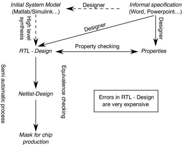
Figure 1: Digital system design flow

One possibility is to use high level synthesis for generating a register transfer level (RTL) design which describes the flow of signals between registers in terms of a hardware description language [4]. But this is rarely used in practise as it does constrain the freedom of the design. Instead, designers manually create the RTL design in a hardware desription language . Concurrently, intended behavior specified by the informal specification is formalized by formal properties. Automatic tools are used to ensure that the RTL design fulfills these conditions.

After passing property checking a netlist is generated semi-automatically from the RTL. The latter is used to derive the actual layout of the chip mask. The validation that different circuit descriptions arising from the last two steps emit the same behaviour, is called equivalence checking. Since this can be handled accurately, setting of the RTL design is the most crucial part. Errors at this level may become very expensive, as they may lead to unusable chip masks or even defective prototypes. The present paper is concerned with this critical level.

The ability of checking the validity of a proposed design restricts the design itself: a newly introduced design approach may not be used for an implementation as long as its verification cannot be ensured. In particular, this applies to digital systems consisting of combined logic and arithmetic blocks, which may not be treated with specialised approaches. Here, dedicated methods from computer algebra may lead to more generic procedures, which help to fill the design gap.

1.3 Problem formulation and encoding in algebra

The verification problem is defined by a set of axioms $M$ representing the circuit w. r. t. given decision variables. In addition, a set of statements $P$ represents the property to be checked. For instance, if $M$ models a multiplication unit, a suitable $P$ would be the condition that after a complete cycle the output of $M$ is the product of its inputs.

The question, whether the circuit represented by $M$ fulfills $P$ can be reformulated in the following way: First of all, we may assume, that $M$ is consistent, i. e. there are no contradictions inherent in the axioms, since the axioms describe a circuit. Then the new set of axioms $M\wedge\neg P$ is contradictable if and only if $M$ implies $P$. Hence the desired property $P$ will be proven by showing, that $M\wedge\neg P$ has no valid instance, i. e. one fulfilling the axioms and not the property.

In the following we encode this logical system into a system of algebraic equations in two ways, on word-level and on bit-level. The word-level model will lead to consider Gröbner bases over the ring $\mathbb{Z}_{2^{n}}$ while the bit-level will lead to Gröbner basis over Boolean rings. Here and in the following $\mathbb{Z}_{m}$ denotes the finte ring $\mathbb{Z}/m\mathbb{Z}$ for $m\in\mathbb{Z}\backslash\{0\}$.

1.3.1 Word-level encoding

We illustrate, how the problem of formal verification can be encoded in a system of algebraic equations using polynomials over the ring $\mathbb{Z}_{2^{n}}$. Let $n$ be the word length of the circuit, i. e. the number of bits used by each signal (in typical applications we have $n\in\{16,32,64\}$). Then the RTL description displayed in Figure 2(a) is equivalent to the following set of algebraic equations

$$M=\{b+c=d,\;a\cdot d=e\}$$ (1)

where $b+c-d,a\cdot d-e$ are polynomials in $\mathbb{Z}_{2^{n}}[a,b,c,d,e,f]$. Of course, the two equations in $M$ are equivalent to $a\cdot(b+c)=e$, but in general the latter input-output form is infeasible due to its complexity. Also, there can be more than one output per block and only some of these outputs may be used further.

For example, Figure 2(b) presents the property

$$P=\{b=0,\;a\cdot c=f\}.$$ (2)

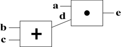
(a) RTL diagram

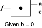
(b) Property

Figure 2: RTL design and property

In this case, the statement that $M$ implies $P$ is equivalent to the assertion that $M\cup P\cup\{f\neq e\}$ has no solution. Since the set $\{f\neq e\}$ is not a closed algebraic set, we replace $f\neq e$ by $s\cdot(f-e)=2^{n-1}$, where $s$ is a new variable. Indeed, it is easy to see that a value $s\in\mathbb{Z}_{2^{n}}$ fulfills this equation if and only if $f\neq e$ (since the ring $\mathbb{Z}_{2^{n}}$ has zero-divisors, $f\neq e$ cannot be encoded by $s(f-e)=1$). Let $I$ be the ideal $\left\langle\{b+c-d,a\cdot d-e,\;\;b,a\cdot c-f,\;\;s\cdot(f-e)-2^{n-1}\}\right\rangle$ in $\mathbb{Z}_{2^{n}}[a,b,c,d,e,f,s]$. Then the question reduces to the question whether

$$\operatorname{V}(I):=\{(a,b,c,d,e,f,s)\in\mathbb{Z}_{2^{n}}^{7}\,|\,p(a,b,c,d,e,f,s)=0,\;\text{for all}\;p\in I\}$$

is empty. There are no solutions for the ideal $I$ (i. e. $\operatorname{V}(I)=\emptyset$) if and only if $M\wedge\neg P$ is contradictable, that is, $P$ is satisfied by $M$.

One way of tackling this problem is to compute a Gröbner basis of $I$ in the ring $R/I_{0}$, where $I_{0}$ denotes the ideal of vanishing polynomials in $R$, i. e. polynomials evaluating to zero at any point of $\mathbb{Z}_{2^{n}}^{7}$. Due to the zerodivisors in this ring the ideal $I_{0}$ has more structure than in the finite field case and even its Gröbner basis can become huge (cf. [5]).

1.3.2 Bit-level encoding

An alternative approach is to encode the problem at the bit-level, that is, as polynomials over $\mathbb{Z}_{2}$. This approach is based on the fact that every value of $x$ in $\mathbb{Z}_{2^{n}}$ can be encoded uniquely to the base 2, i. e. in its bits:

$$x=x_{0}+x_{1}2+\dots+x_{n-1}2^{n-1},\,x_{i}\in\{0,1\}\,\mbox{.}$$ (3)

In the example above we can express each variable $a,b,c,d,e,f$ analogously to equation (3) with new variables $a_{i},b_{i},c_{i},d_{i},e_{i},f_{i}\in\{0,1\},i=0,\dots,n-1$. Then equation (1) and equation (2) must be rewritten, which yields $n$ equations for each of them. Gathering all corresponding polynomials and adding the polynomial $\prod\left(1-f_{i}+e_{i}\right)$, which is equivalent to $f\neq e$, we obtain an ideal $I$ over $R:=\mathbb{Z}_{2}[a_{0},\ldots,f_{n-1}]$ in $6\,n$ variables.

For instance, the bits $p_{0},\dots,p_{n-1}\in\{0,1\}$ of the product $p=a\cdot b$ are given by equations $p_{j}=a_{j}\cdot b_{0}+\sum_{i=0}^{j-1}(a_{i}\cdot b_{j-i}+t_{i,j-i})$ over $\mathbb{Z}_{2}$, where the $t_{k,l}$ mark rather complicated bit-level expressions in the $s_{k,l}\in\{0,1\}$, which fulfill $p_{k}+s_{k,1}2+\dots+s_{k,n-1}2^{n-1}=a_{k}\cdot b_{0}+\sum_{i=0}^{k-1}(a_{i}\cdot b_{k-i}+s_{i,k-i})$ in $\mathbb{Z}_{2^{n}}$. For example, for $n=4$, we get

$$p_{3} = a_{3}\,b_{0}+a_{2}\,b_{1}+a_{1}\,b_{2}+a_{0}\,b_{3}+a_{2}\,a_{1}\,a_{0}\,b_{1}\,b_{0}+$$

$$\quad a_{2}\,a_{1}\,b_{1}\,b_{0}+a_{2}\,a_{0}\,b_{2}\,b_{0}+a_{1}\,a_{0}\,b_{2}\,b_{1}\,b_{0}+a_{1}\,a_{0}\,b_{2}\,b_{1}+a_{1}\,a_{0}\,b_{1}\,b_{0}$$

$$p_{2} = a_{2}\,b_{0}+a_{1}\,b_{1}+a_{0}\,b_{2}\ +a_{1}\,a_{0}\,b_{1}\,b_{0}$$

$$p_{1} = a_{1}\,b_{0}+a_{0}\,b_{1}$$

$$p_{0} = a_{0}\,b_{0}$$

Again let $I_{0}$ be the ideal of vanishing polynomials in $R$. In this case, the ideal $I_{0}$ is generated by the field equations $x^{2}-x=0$ for every variable $x$. Now we compute a Gröbner basis of $I$ in the ring $R/I_{0}$. In this ring every ideal is principal (cf. Theorem 60) and hence its reduced Gröbner basis will consist of just one polynomial. Moreover, $I=\left\langle 1\right\rangle$ if and only if its reduced Gröbner basis is $\{1\}$ and this is equivalent to the zero set of all polynomials in $I$ being empty, and therefore if and only if the property $P$ holds.

1.3.3 Modelling advantages and disadvantages

Both modelling approaches presented in section 1.3.1 and section 1.3.2 have strengths and weakenesses. On the one hand, the word-level formulation of verification problems as polynomial systems over $\mathbb{Z}_{2^{n}}$ leads to fewer variables and equations. The equations of arithmetic blocks, like multiplier and adder blocks, are given in a natural and human readable way. However, not all formulæ on word-level (for example bitwise and, or, and exclusive-or) may be coded by polynomial equations. Therefore, full strength will need bit-level encoding of some variables. Another drawback are the coefficients from $\mathbb{Z}_{2^{n}}$, which is a ring with zero-divisors and not a field. Hence, one cannot rely on valueable properties of fields, like the algebraic closure.

Since $\mathbb{Z}_{2}$ is a field, these restrictions do not exists for polynomials over $\mathbb{Z}_{2}$, which can be used for formulation of arbitrary bit-level equations. Moreover, since the coefficients are restricted to be one or zero, they need not to be stored at all. Hence, a specialised data structure is possible, which is tailored to suit this application task. On the other hand, contrary to the word-level case, bit-level formulations carry many variables and equations. The number of them may grow exponentially even for some applications which can be handled easily over $\mathbb{Z}_{2^{n}}$.

As a result from these considerations, research was done for both approaches. In the following, we present the different strategies and solutions for both, the word-level and bit-level approach, in the appropriate algebraic setting.

2 Standard bases over rings

2.1 Basic definitions

In this paragraph we outline the general theory of standard bases for ideals or modules over a polynomial ring $C[x_{1},\dots,x_{n}]$ where $C$ is any commutative Noetherian ring with 1. We do not require that the monomial ordering is a well-ordering, that is we treat the case of standard bases in the localization of $C[x_{1},\dots,x_{n}]$ as well (for a full treatment cf. [6]). Gröbner bases over $C[x_{1},\dots,x_{n}]$ (i. e. the case of well-orderings) have been treated previously (cf. [7, 8]) but never for non well-orderings. Since we are mainly interested in the case $C=\mathbb{Z}_{2^{n}}$ we allow $C$ to have zero-divisors. Moreover, since we are interested in practical application to real world formal verification problems, we have to develop the theory for $C=\mathbb{Z}_{m}$ with special care. The ring $\mathbb{Z}_{m}$ allows special algorithms which dramatically improves the performance of Gröbner bases computations against generic implementations for general rings.

We recall some algebraic basics, including classical notions for the treatment of polynomial systems, as well as basic definitions and results from computational algebra. For an exhaustive textbook about the subject, when the ground ring $C$ is a field, we refer to [9] and the references therein.

Let $C[\mathbf{x}]=C[x_{1},\dots,x_{n}]$ be the polynomial ring over $C$, equipped with an arbitrary monomial ordering $<$, i. e. global (well-ordering), local or mixed (cf. [9]). Further $C[\mathbf{x}]_{<}$ denotes the localization of $C[\mathbf{x}]$ by the multiplicatively closed set

$$S_{<}=\{f\in C[\mathbf{x}]\backslash\{0\}~{}|~{}\operatorname{LM}\left(f\right)=1\wedge\operatorname{LC}\left(f\right)\in C^{*}\},$$

where $C^{*}$ is the group of units of $C$ and $\operatorname{LM}$ respectively $\operatorname{LC}$ denote the leading monomial respectively the leading coefficient w.r.t. $<$, as defined in [9]. Then

$$R:=C[\mathbf{x}]_{<}=\left\{\left.\frac{f}{g}~{}\right|~{}f\in C[\mathbf{x}],g\in S_{<}\right\}.$$

Also, consider a partition of the ring variables $\{\mathbf{x},\mathbf{y}\}=\{x_{1},\dots,x_{n},y_{1},\dots,y_{m}\}$. A monomial ordering over $C[\mathbf{x},\mathbf{y}]$ is called an elimination ordering for $\mathbf{x}$, if $x_{i}>t$ for each $i$ and for every monomial $t$ in $C[\mathbf{y}]$.

Definition 1

Let $I\subset R=C[\mathbf{x}]_{<}$ be an ideal and $f$ an element in $R$. Choose $u\in S_{<}$ such that $\operatorname{LC}\left(u\right)=1$ and $u\cdot f$ is a polynomial $a_{0}\cdot\mathbf{x}^{\alpha_{0}}+\dots+a_{n}\cdot\mathbf{x}^{\alpha_{n}}\in C[\mathbf{x}]$ with $a_{0}\neq 0$ and $x^{\alpha_{0}}>x^{\alpha_{i}}$ for all $i\neq 0$ with $a_{i}\neq 0$ (which is always possible). Then we define

$$\operatorname{LT}\left(f\right) =a_{0}\cdot\mathbf{x}^{\alpha_{0}} f$$ leading term of

$$\operatorname{LM}\left(f\right) =\mathbf{x}^{\alpha_{0}} f$$ leading monomial of

$$\operatorname{LC}\left(f\right) =a_{0} f$$ leading coefficient of

$$\operatorname{LE}\left(f\right) =\alpha_{0} f$$ leading exponent of

$$\operatorname{L}\left(I\right) =\left\langle\operatorname{LT}\left(f\right)~{}|~{}f\in I\right\rangle_{C[\mathbf{x}]} I$$ leading ideal of

$$\operatorname{LM}\left(I\right) =\left\langle\operatorname{LM}\left(f\right)~{}|~{}f\in I\right\rangle_{C[\mathbf{x}]} I$$ leading monomials ideal of

$$\operatorname{V}(I) =\{\mathbf{x}~{}|~{}\forall f\in I:f(\mathbf{x})=0\} I$$ common zeroes or variety of

$$\operatorname{I}(V) =\{f~{}|~{}\forall\mathbf{x}\in V:f(\mathbf{x})=0\} V\subset C^{n}$$ vanishing ideal of

$$\operatorname{supp}(f) =\{\mathbf{x}^{\alpha_{i}}~{}|~{}a_{i}\neq 0\} f$$ support of

$$\operatorname{tail}(f) =f-\operatorname{LT}\left(f\right) f$$ tail of

If the monomial order $<$ is global then $u=1$. If $<$ is not global the leading coefficients and the leading terms are well defined, independent of the choice of $u$.

Definition 2

Let $I\subset R=C[\mathbf{x}]_{<}$ be an ideal. A finite set $G\subset R$ is called a standard basis of $I$ if

$$G\subset I\text{ and }\operatorname{L}\left(I\right)=\operatorname{L}\left(G\right).$$

That is, $G$ is a standard basis, if the leading terms of $G$ generate the leading ideal of $I$. $G$ is called a strong standard basis if, for any $f\in I\backslash\{0\}$, there exists a $g\in G$ satisfying $\operatorname{LT}\left(g\right)|\operatorname{LT}\left(f\right)$. If $<$ is global we will call standard bases also Gröbner bases. A finite set $G\subset R$ is called standard resp. Gröbner basis, if $G$ is a standard resp. Gröbner basis of $\left\langle G\right\rangle_{R}$, the ideal generated by $G$.

Remark 3

If $C$ is a field, than $\operatorname{L}\left(I\right)=\operatorname{LM}\left(I\right)$, but due to non-invertible coefficients, in general only $\operatorname{L}\left(I\right)\subset\operatorname{LM}\left(I\right)$ holds.

Next, the notion of $t$-representations is introduced, as formulated in [10]. While this notion is mostly equivalent to using syzygies, it helps to understand the correctness of the algorithms.

Definition 4 ($t$-representation)

Let $t$ be a monomial and consider elements

$$f,g_{1},\ldots,g_{m},h_{1},\ldots,h_{m}\in C[\mathbf{x}]_{<}=R$$

with $f=\sum_{i=1}^{m}h_{i}\cdot g_{i}$. Then the sum is called a $t$-representation of $f$ with respect to $g_{1},\ldots,g_{m}$ if

$$\operatorname{LM}(h_{i}\cdot g_{i})\leq t\text{ for all }i\text{ with }h_{i}\cdot g_{i}\neq 0\,\mbox{.}$$

Example 5

Let the monomials of $C[x,y]$ be lexicographically ordered ($x>y$) and $g_{1}=x^{2},g_{2}=x^{5}-y,f=y$. Then $f=x^{3}g_{1}-g_{2}$ is a $x^{5}y^{5}$-representation of $f$.

Notation 6

Given a representation $p=\sum_{i=1}^{m}h_{i}\cdot f_{i}$ with respect to $f_{1},\ldots f_{m}$, we may shortly say that $p$ has a nontrivial $t$-representation, if a $t$-representation of $p$ exists with

$$t<\max\{\operatorname{LM}(h_{i}\cdot f_{i})|h_{i}\cdot f_{i}\neq 0\}.$$

Note that there exists no $t$-representations with $t<\operatorname{LM}(p)$. Further, we say that an arbitrary $g$ has a standard representation with respect to $\{f_{i}\}$, if it has a $\operatorname{LM}\left(g\right)$-representation.

2.2 Normal forms

Definition 7

Let $\mathcal{G}$ be the set of all finite subsets $G$ of $R=C[\mathbf{x}]_{<}$. A map

$$\operatorname{NF}:R\times\mathcal{G}\to R,(f,G)\mapsto\operatorname{NF}\left(\left.f\,\right|\,G\right)$$

1. is called a normal form on $R$ if, for all $G\in\mathcal{G}$,

   1. $\operatorname{NF}\left(\left.0\,\right|\,G\right)=0$,

   and, for all $f\in R$ and $G\in\mathcal{G}$,

   1. $\operatorname{NF}\left(\left.f\,\right|\,G\right)\neq 0\Rightarrow\operatorname{LT}\left(\operatorname{NF}\left(\left.f\,\right|\,G\right)\right)\not\in\operatorname{L}\left(G\right)$ and

   2. $r:=f-\operatorname{NF}\left(\left.f\,\right|\,G\right)$ has a standard representation with respect to $G$.

2. is called a weak normal form, if instead of $r$ we just require that the polynomial $r^{\prime}=uf-\operatorname{NF}\left(\left.f\,\right|\,G\right)$ for a unit $u\in{R}^{*}$ has a standard representation with respect to $G$.

3. is called polynomial weak normal form if it is a weak normal form and whenever $f\in C[\mathbf{x}]$ and $G\subset C[\mathbf{x}]$, there exists a unit $u\in{R}^{*}\cap C[\mathbf{x}]$, such that $uf-\operatorname{NF}\left(\left.f\,\right|\,G\right)$ has a standard representation $\sum_{i=1}^{n}a_{i}g_{i}$ w.r.t. $G=\{g_{1},\dots,g_{n}\}$ with $a_{i}\in C[\mathbf{x}]$.

Remark 8

Polynomial weak normal forms exists for arbitrary Noetherian rings and are computable if linear equations over $C$ are solvable (Theorem 11).

Definition 9

We call a normal form $\operatorname{NF}\left(\left.\cdot\,\right|\,\cdot\right)$ reduced, if for all $f\in R$ and $G\in\mathcal{G}$ the leading terms of elements from $G$ do not divide any term of $\operatorname{NF}\left(\left.f\,\right|\,G\right)$. Further we call $G$ a reduced Gröbner basis, if no term from $\operatorname{tail}(g)$ for any $g\in G$ is divisible by a leading term of an element of $G$.

Now we introduce an algorithm for computing a polynomial weak normal form for any monomial ordering, given we are able to solve an arbitrary linear equation in the coefficient ring $C$. To ensure correctness and termination we need to introduce the concept of the $\operatorname{ecart}$ of a polynomial.

Definition 10

Let $f\in R\backslash\{0\}$ be a polynomial. Then the ecart is defined by

$$\operatorname{ecart}f=\deg f-\deg\operatorname{LM}\left(f\right).$$

We introduce a monomial order $<_{h}$ on $C[t,\mathbf{x}]$ where $t$ is a new variable via

$$t^{p}\mathbf{x}^{\alpha}<_{h}t^{q}\mathbf{x}^{\beta}:\Longleftrightarrow \hskip 8.4ptp+{\left\lvert\alpha\right\rvert}<q+{\left\lvert\beta\right\rvert}\text{ or }$$

$$\left(p+{\left\lvert\alpha\right\rvert}=q+{\left\lvert\beta\right\rvert}\text{ and }\mathbf{x}^{\alpha}<\mathbf{x}^{\beta}\right).$$

This is a well-ordering as there are only finitely many monomials with a given total degree.

Algorithm 1 Calculating a normal form over coefficient rings

0:  $f\in R$ a polynomial, $G\subset R$ finite, $>$ a monomial ordering

0:  A normal form of $f$

  $T:=G$

  while $f\neq 0$ and $\operatorname{LT}\left(f\right)\in\operatorname{L}\left(T\right)$ do

     solve $\operatorname{LT}\left(f\right)=\sum\limits_{i=1}^{s}c_{i}\,\mathbf{x}^{\alpha_{i}}\operatorname{LT}\left(g_{i}\right)$

with $\mathbf{x}^{\beta_{i}}\operatorname{LM}\left(g_{i}\right)=\operatorname{LM}\left(f\right)$,

$g_{i}\in T$ and $\max\{\operatorname{ecart}g_{i}\}$ minimal

     if $\max\{\operatorname{ecart}g_{i}\}>0$ then

        $T:=T\cup\{f\}$

     $f:=f-\sum\limits_{i=1}^{s}c_{i}\,\mathbf{x}^{\beta_{i}}g_{i}$

  return  $f$

Theorem 11

The Algorithm 1 terminates and computes a norm form, if we can solve linear equation in the coefficient ring $C$.

Remark 12

In many cases it is not necessary to solve linear equations during the normal form computation. These include coefficient fields (the classical case), weak 1-factorial rings or principal ideal domains. The latter case was already treated in [7]. Further cases can also be computed without solving linear equations if we require $G$ to be a strong Gröbner basis.

2.2.1 Weak factorial rings

In rings with zero-divisors we have in general no decomposition into irreducible elements. For example in $\mathbb{Z}_{12}$ we have $6=3\cdot 6=3\cdot 3\cdot 6=\dots$. Therefore the concept of factoriality does not make sense. But there exists a notion of weak factorial rings where every element can be written as $a=n\cdot a_{1}^{r_{1}}\cdot\dots\cdot a_{k}^{r_{k}},r_{i}\geq 0$ ($n$ not necessarily a unit), such that $a\,|\,b=m\cdot a_{1}^{s_{1}}\cdot\dots\cdot a_{k}^{s_{k}}$ iff $r_{i}\leq s_{i}$. This will be formalized below.

Let $C$ be a commutative Noetherian ring with $1$ and ${C}^{*}$ the group of units. Denote further by $\operatorname{N}\left(C\right)=\{a\in C~{}|~{}\exists b\neq 0~{}:~{}a\cdot b=0\}$, the zero-divisors and by $\operatorname{NE}\left(C\right)=C\backslash{C}^{*}$ the non-units in $C$.

Definition 13

An element factorization $(\nu,P)$ or just $\nu$ for a ring $C$ consists of a subset $P\subset\operatorname{NE}\left(C\right)$ and a map $\nu=(\nu_{p})_{p\in P}:C\to\mathbb{N}^{P}$, $\nu_{p}:C\to\mathbb{N}$, such that for all $a\in C$ there exists an element $n\in C$ with

$$a=n\cdot\prod_{p\in P}p^{\nu_{p}(a)}=:n\cdot\mathbf{p}^{\nu(a)}$$

and $\nu_{p}(a)\neq 0$ only for finitely many $p\in P$.

A ring $C$ with an element factorization $\nu$ is called $P$-weak factorial or just weak factorial if, for all $a,b\in C$

$$a~{}|~{}b\Longleftrightarrow\nu(a)\leq\nu(b).$$

That is, divisibility in $C$ is given by the natural order relation of $\mathbb{N}^{P}$. If we want to emphasise the number of elements in $P$ (elements in $P$ are also called “primes”), we say weak ${\left\lvert P\right\rvert}$-factorial ring where ${\left\lvert P\right\rvert}$ is the cardinality of $P$.

Example 14

1. If $C$ is a factorial domain and $P$ the set of irreducible elements then $C$ is $P$-weak factorial.

2. The ring of integers modulo a power of a prime number $p$ is a weak 1-factorial ring with $P=\{p\}$.

3. The ring $\mathbb{Z}_{m}$ is weak factorial with $P=\{p\in\mathbb{P}~{}|~{}p~{}|~{}m\}$, where $\mathbb{P}$ denotes the set of prime numbers.

4. The ring $\mathbb{Z}$ is a weak $\infty$-factorial ring with $P=\mathbb{P}$ and $\nu=\nu^{\mathbb{Z}}$ the map which associate to $a\in\mathbb{Z}$ the exponents of the prime decomposition of $a$.

5. The ring $\mathbb{K}[[x]]$, $\mathbb{K}$ a field, is weak factorial with $P=\{x\}$.

Remark 15

For the case of $\mathbb{Z}_{m}$ with $m=p_{1}^{e_{1}}\cdots p_{n}^{e_{n}}$, we define $\nu$ as

$$\nu_{p_{i}}(\underline{a}):=\nu_{i}(a)=\min\{\nu^{\mathbb{Z}}_{p_{i}}(a),e_{i}\}$$

where $a\in\mathbb{Z}$ represents $\underline{a}\in\mathbb{Z}_{m}$. E.g. in $\mathbb{Z}_{12}$ we have $12=2^{2}\cdot 3^{1}$ and therefore $\nu_{3}(9)=1$ and $9=3\cdot 3=n\cdot 3^{1}$. Further in this case $\nu$ has the following properties:

Proposition 16

Let $\nu$ be defined for $\mathbb{Z}_{m}$ as in Remark 15. Then we have

1. $\nu$ is well-defined, that is $\nu(a)=\nu(a+k\cdot m)$ for all $a,k,m\in\mathbb{Z}$.

2. $\nu$ is saturated multiplicative, that is $\nu_{i}(a\cdot b)=\min\{\nu_{i}(a)\cdot\nu_{i}(b),e_{i}\}$,

3. $\nu_{i}(a+b)=0$ if $\nu_{i}(a)>0$ and $\nu_{i}(b)=0$,

4. $\nu(a)=0\Leftrightarrow\underline{a}\in{\mathbb{Z}_{m}}^{*}$ and

5. $\nu$ is nice weak factorial, that is, $\forall\underline{a}\in\mathbb{Z}_{m}~{}\exists\underline{u}\in{\mathbb{Z}_{m}}^{*}\,:\,\underline{a}=\underline{u}\cdot\mathbf{p}^{\nu(\underline{a})}$.

[Proof.] The first four properties follow easily from the valuation properties of $\mathbb{Z}$ with $\nu^{\mathbb{Z}}$. For the last one let $\underline{a}=\underline{n}\cdot\mathbf{p}^{\nu(\underline{a})}$. At first notice, that $\nu_{p_{i}}(\underline{n})>0$ is only possible, if $\nu_{p_{i}}(\underline{a})=e_{i}$. Hence consider

$$u=n+\frac{m}{\mathbf{p}^{\nu(a)}}\cdot\mathop{\prod_{e_{i}>0}}_{p_{i}\nmid\,n}p_{i}.$$

Now $\nu(\underline{u})=0$ and therefore $\underline{u}\in{\mathbb{Z}_{m}}^{*}$. Further $\underline{u}\cdot\mathbf{p}^{\nu(\underline{a})}=\underline{a}$.

Remark 17

One can show that in our definition the elements of $P$ are irreducible and that $C$ is a weak unique factorization ring (UFR) in the sense of Agargün [11] and therefore a generalisation of the notions from Bouvier-Galovich [12, 13] and Fletcher [14] (cf. [11]). Nevertheless we prefer our definition, as it emphasis the divisibility relation.

Remark 18

If $C$ is a principal ideal ring, then it is isomorphic to a finite product [15] of principal ideal domains, hence factorial domains, and finite-chain rings (cf. [15]), which are weak 1-factorial. Therefore we can compute Gröbner basis in polynomials rings over the factors and lift them to $C[\mathbf{x}]$. This is described in the work of G. Norton and A. Salagean [16]. Below we show that computation in the ring itself is feasible.

Definition 19

Let $C$ be a weak factorial ring and $a_{1},\dots,a_{n}\in C$. Then we define (with $\max,\min$ component-wise)

$$\operatorname{gcd}\left(a_{1},\dots,a_{n}\right) =\mathbf{p}^{\min\{\nu(a_{1}),\dots,\nu(a_{n})\}}\quad\text{and}$$

$$\operatorname{lcm}\left(a_{1},\dots,a_{n}\right) =\mathbf{p}^{\max\{\nu(a_{1}),\dots,\nu(a_{n})\}}.$$

Remark 20

This definition of $\gcd$ and $\operatorname{lcm}$ fulfills the universal properties of the greatest common divisor and the least common multiple. But notice that, for arbitrary rings, the $\gcd$ and $\operatorname{lcm}$ are not unique up to units. However, in the case of $\mathbb{Z}_{m}$ this holds:

$$a|b\wedge b|a\Rightarrow\exists u\in{\mathbb{Z}_{m}}^{*}~{}:~{}a=u\cdot b.$$

Lemma 21

Let $C$ be a weak factorial principal ring. Then

$$\left\langle a_{1},\dots,a_{n}\right\rangle =\left\langle\operatorname{gcd}\left(a_{1},\dots,a_{n}\right)\right\rangle,$$

$$\left\langle a_{1}\right\rangle\cap\dots\cap\left\langle a_{n}\right\rangle =\left\langle\operatorname{lcm}\left(a_{1},\dots,a_{n}\right)\right\rangle.$$

[Proof.] Follows directly from the definition of weak factorial and $\gcd$, respectively $\operatorname{lcm}$, and their universal properties.

Lemma 22

Let $C$ be a weak 1-factorial principal ring with prime $\eta$ and let $c,a_{1},\dots,a_{s}\in C\backslash\{0\}$. Then the following are equivalent.

• The equation $c=a_{1}x_{1}+\dots+a_{s}x_{s}$ is solvable.

• There exists an $j\in\{1,\dots,s\}$ and $x\in C$, such that $c=a_{j}x$, i. e. $a_{j}|c$.

[Proof.] The first statement is equivalent to

$$c\in\left\langle a_{1},\dots,a_{n}\right\rangle$$

$$\Leftrightarrow \operatorname{gcd}\left(a_{1},\dots,a_{n}\right)~{}|~{}c$$

$$\Leftrightarrow \min\left\{\nu(a_{1}),\dots,\nu(a_{n})\right\}\leq\nu(c)$$

$$\Leftrightarrow \exists a_{i}~{}:~{}\nu(a_{i})\leq\nu(c),\text{ as }\operatorname{Im}\left(\nu\right)\subset\mathbb{N}$$

$$\Leftrightarrow c\in\left\langle a_{i}\right\rangle$$

which is equivalent to the second statement.

Corollary 23

Let $C$ be a weak 1-factorial principal ring. Then, solving linear equations over $C$ can be reduced to tests for divisibility. Moreover, every standard basis over $C[\mathbf{x}]_{<}$ is a strong standard basis.

2.3 Computing standard bases

Let $C$ be a commutative Noetherian ring with $1$.

Definition 24

Let $R$ be a ring and $A\in R^{s\times t}$ a matrix considered as a linear map $R^{s}\to R^{t}$. The kernel of $A$ is a submodule of $R^{s}$. It is called the syzygy module of $A$. If $A=(f_{1},f_{2},\dots,f_{s})\in R^{s\times 1}$, then

$$\operatorname{Syz}\left(f_{1},\dots,f_{s}\right)=\ker(A)=\{(h_{1},\dots,h_{s})\in R^{s}~{}|~{}\sum h_{i}f_{i}=0\}.$$

Theorem 25

(Buchberger’s criterion) Let $I\subset R=C[\mathbf{x}]_{<}$ be an ideal and $G=\{g_{1},\dots,g_{s}\}\subset I$. Further let $\operatorname{NF}\left(\left.-\,\right|\,G\right)$ be a weak normal form on $R$ with respect to $G$. Then the following statements are equivalent:

1. $G$ is a standard basis of $I$.

2. $\operatorname{NF}\left(\left.f\,\right|\,G\right)=0$ for all $f\in I$.

3. Each $f\in I$ has a standard representation with respect to $G$.

4. $G$ generates $I$ and for every element $h$ with

   $$h\in{\operatorname{Syz}\left(\operatorname{LT}\left(g_{i}\right)|i=1,\dots,s\right)},$$

   $\operatorname{NF}\left(\left.h_{1}g_{1}+\dots+h_{s}g_{s}\,\right|\,G\right)=0$.

[Proof.] The implications $1\Rightarrow 2\Rightarrow 3\Rightarrow 4\Rightarrow 1$ can be shown as in the classic case. The classical proof can be found either in [9] (general orderings) or in [7] (global orderings).

To specialize further for the case of weak factorial principal rings we modify the classical notion of an $s$-polynomial.

Definition 26

Let $f,g\in R\backslash\{0\}$. We define the $s$-polynomial of $f$ and $g$ to be

$$\operatorname{spoly}\left(f,g\right):=\frac{\operatorname{lcm}\left(\operatorname{LT}\left(f\right),\operatorname{LT}\left(g\right)\right)}{\operatorname{LT}\left(f\right)}f-\frac{\operatorname{lcm}\left(\operatorname{LT}\left(f\right),\operatorname{LT}\left(g\right)\right)}{\operatorname{LT}\left(g\right)}g.$$

Remark 27

This definition is not equivalent to

$$\operatorname{spoly}_{r}\left(f,g\right)=\\ \operatorname{LC}\left(g\right)\frac{\operatorname{lcm}\left(\operatorname{LM}\left(f\right),\operatorname{LM}\left(g\right)\right)}{\operatorname{LM}\left(f\right)}f-\operatorname{LC}\left(f\right)\frac{\operatorname{lcm}\left(\operatorname{LM}\left(f\right),\operatorname{LM}\left(g\right)\right)}{\operatorname{LM}\left(g\right)}g.$$

For example let $f=2\,x-2\,y,g=2\,y-z$ in $\mathbb{Z}_{4}[x,y,z]$. Then we get $\operatorname{spoly}_{r}\left(f,g\right)=x\,z\neq-2\,y+z\,x=\operatorname{spoly}\left(f,g\right)$. That is, we can loose terms just by multiplying with a constant, e. g. if $2\,x+y\in I$ for some ideal $I$, then $2\,y\in\operatorname{L}\left(I\right)$. Therefore we have to look for further generators of the syzygies, the classical $s$-polynomials are not sufficient.

Definition 28

Let $C$ be a principal ring and $a\in C$. The annihilator of $a$, $\text{Ann}(a)=\{n\in C~{}|~{}a\cdot n=0\}$ is an ideal in $C$ and is hence generated by one element, which we denote by $\operatorname{NT}\left(a\right)$.

Due to zero-divisors we define the $s$-polynomial also for pairs $(f,g)$ with one component being $0$.

Definition 29

Let $f\in R\backslash\{0\}$. We define the extended s-polynomial of $f$ to be

$$\operatorname{spoly}\left(0,f\right)=\operatorname{spoly}\left(f,0\right):=\operatorname{NT}\left(\operatorname{LC}\left(f\right)\right)\cdot f.$$

Algorithm 2 Computes a standard basis of $I$

0:   $I$ a finite set of polynomials, $>$ a monomial ordering, $\operatorname{NF}$ a weak normal form

0:  $G$ is a standard basis of $I$

  $G:=I$

  $P:=\{(f,g)~{}|~{}f,g\in S,f\neq g\}\cup\{(0,f)~{}|~{}f\in G\}$, the pair set

  while $P\neq\emptyset$ do

     choose $(f,g)\in P$

     $P:=P\backslash\{(f,g)\}$

     $h:=\operatorname{NF}\left(\left.\operatorname{spoly}\left(f,g\right)\,\right|\,G\right)$

     if $h\neq 0$ then

        $P:=P\cup\{(h,f)\,|\,f\in G\}\cup\{(0,h)\}$

        $G:=G\cup\{h\}$

  return  $G$

2.3.1 Buchberger’s criterion and the syzygy theorem

In the following we assume $C$ to be a weak factorial principal ring. Termination of Algorithm 2 is an easy consequence of the Noetherian property of the ring $R$. To present the theorem, which implies the correctness of Algorithm 2 we need to introduce some terminology. We fix a set of generators $G=\{f_{0},f_{1},\dots,f_{k}\}$ of an ideal $I$ with $f_{0}=0$.

First assume that a set $J\subset\{(i,j)~{}|~{}0\leq j<i\leq k\}$ is given with

$$\operatorname{NF}\left(\left.\operatorname{spoly}\left(f_{i},f_{j}\right)\,\right|\,G\right)=0\text{ for }(i,j)\in J.$$

For $0\leq i<j\leq k$ let $\operatorname{LT}\left(f_{i}\right)=c_{i}\mathbf{x}^{\alpha}_{i}$ and define:

$$m_{ji} =\frac{\operatorname{lcm}\left(c_{i},c_{j}\right)}{c_{i}}\cdot\frac{\operatorname{lcm}\left(\mathbf{x}^{\alpha_{i}},\mathbf{x}^{\alpha_{j}}\right)}{\mathbf{x}^{\alpha_{i}}}=\frac{\operatorname{lcm}\left(\operatorname{LT}\left(f_{i}\right),\operatorname{LT}\left(f_{j}\right)\right)}{\operatorname{LT}\left(f_{i}\right)}$$

$$m_{0i} =\operatorname{NT}\left(c_{i}\right)$$

$$\operatorname{spoly}\left(f_{i},f_{j}\right) =m_{ji}f_{i}-m_{ij}f_{j}$$

$$\operatorname{spoly}\left(f_{i},f_{0}\right) =m_{0i}f_{i}\text{ as }f_{0}=0\text{ (set also }m_{i0}=0\text{)}$$

$$\operatorname{spoly}\left(f_{i},f_{j}\right) =\sum_{\nu=1}^{k}a_{\nu}^{(ij)}f_{\nu}\text{ the standard representation for }(i,j)\in J$$

$$s_{ij} =m_{ji}\mathbf{e}_{i}-m_{ij}\mathbf{e}_{j}-\sum_{\nu=1}^{k}a_{\nu}^{(ij)}\mathbf{e}_{\nu}\in\operatorname{Syz}\left(I\right)\text{ for }(i,j)\in J$$

The elements $m_{0i}$ and $s_{i0}$ correspond to the new $s$-polynomials, which occur due to zero divisors.

Theorem 30 (Buchberger’s criterion)

Let $G=\{f_{0},f_{1},\dots,f_{k}\}$ be a set of generators of $I\subset R$ with $f_{0}=0$. Further let $J\subset\{(i,j)~{}|~{}0\leq i<j\leq k\}$ be such that $\left\langle{m_{ij}\mathbf{e}_{j}~{}|~{}(i,j)\in J}\right\rangle=\left\langle{m_{ij}\mathbf{e}_{j}~{}|~{}0\leq j<i\leq k}\right\rangle$. If

$$\operatorname{NF}\left(\left.\operatorname{spoly}\left(f_{i},f_{j}\right)\,\right|\,G_{ij}\right)=0\text{ for }(i,j)\in J$$

and some $G_{ij}\subset G$ then

1. $G$ is a standard basis of $I$ (Buchberger’s criterion) and

2. $S:=\{s_{ij}~{}|~{}(i,j)\in J\}$ generates $\operatorname{Syz}\left(I\right)$.

For a proof we refer to [6].

Remark 31

The set $S$ is a standard basis of $\operatorname{Syz}\left(I\right)$ with respect to the Schreyer ordering (definition of the Schreyer ordering cf. [9]).

Corollary 32

Algorithm 2 terminates and is correct.

Remark 33

If $f$ and $I$ are polynomial and if $\operatorname{NF}$ is a polynomial weak normal form in Algorithm 2 than $G$ is a standard basis of $\left\langle I\right\rangle_{R}$ consisting of polynomials.

Also, the $t$-representations of Definition 4 can be utilised for a standard basis test as given below.

Theorem 34

Let $F=(0,f_{1},\ldots,f_{k})$, $f_{i}\in C[\mathbf{x}]$, be a polynomial system. If $\operatorname{spoly}\left(f,g\right)$ has a nontrivial $t$-representation w. r. t. $F$ for each $f,g\in F$, then $F$ is a Gröbner basis.

[Proof.] The theorem can be proved similar as in [10]. A more sophisticated version of this theorem can be formulated and proven likewise to [9, p. 142].

2.3.2 Criteria for $s$-polynomials

In order to compute non-trivial standard bases in practise, we like to have criteria to omit unnecessary critical pairs. This improves the time and space requirement of the Buchberger algorithm as in the classical case.

Lemma 35 (Product criterion)

Let $f,g\in R=C[\mathbf{x}]_{<}$ with $\operatorname{LM}\left(f\right)$ and $\operatorname{LM}\left(g\right)$ relatively prime. Further let $\operatorname{LC}\left(f\right)$ and $\operatorname{LC}\left(g\right)$ be a unit, then

$$\operatorname{NF}\left(\left.\operatorname{spoly}\left(f,g\right)\,\right|\,\{f,g\}\right)=0.$$

[Proof.] No change of the classical proof is needed. However, the strong product criterion, which gives an if and only if statement, is not extendable to the general case.

Example 36

The polynomials $4x+y$ and $y^{2}+2\,z\in\mathbb{Z}_{8}[x,y,t]$ will reduce to zero by a sharper product criterion (not given here). In contrast $4\,y+x^{3}+1$ and $x^{5}+2\,x^{2}$ will reduce to $2\,x^{2}$, which is not reducible by either of the polynomials nor their extended $s$-polynomials.

Lemma 37 (Chain criterion)

With the notations of Theorem 30 let $\operatorname{LT}\left(f_{i}\right)=c_{i}\,\mathbf{x}^{\alpha_{i}}$, $\operatorname{LT}\left(f_{j}\right)=c_{j}\,\mathbf{x}^{\alpha_{j}}$, and $\operatorname{LT}\left(f_{l}\right)=c_{l}\,\mathbf{x}^{\alpha_{l}}$ with $i>j>l$. If $c_{j}\,\mathbf{x}^{\alpha_{j}}$ divides $\operatorname{lcm}\left(c_{i}\,\mathbf{x}^{\alpha_{i}},c_{l}\,\mathbf{x}^{\alpha_{l}}\right)$ then $m_{li}\,\mathbf{e}_{i}\in\left\langle m_{ji}\,\mathbf{e}_{i}\right\rangle$. In particular, if $s_{ij},s_{jl}\in S$ then $S\backslash\{s_{il}\}$ is already a standard basis of $\operatorname{Syz}\left(I\right)$ and $S\backslash\{s_{il}\}$ generates $\operatorname{Syz}\left(I\right)$.

[Proof.] The divisibility of $\operatorname{lcm}\left(c_{i}\,\mathbf{x}^{\alpha_{i}},c_{l}\,\mathbf{x}^{\alpha_{l}}\right)$ by $c_{j}\,\mathbf{x}^{\alpha_{j}}$ implies

$$\operatorname{lcm}\left(c_{i}\,\mathbf{x}^{\alpha_{i}},c_{j}\,\mathbf{x}^{\alpha_{j}}\right)~{}|~{}\operatorname{lcm}\left(c_{i}\,\mathbf{x}^{\alpha_{i}},c_{l}\,\mathbf{x}^{\alpha_{l}}\right).$$

Dividing both sides by $c_{i}\,\mathbf{x}^{\alpha_{i}}$ yields $m_{ji}~{}|~{}m_{li}$.

The following criterion is new and quite useful in practise.

Lemma 38

With the notations of Theorem 30 let $\operatorname{LT}\left(f_{i}\right)=c_{i}\,\mathbf{x}^{\alpha_{i}}$ and $\operatorname{LT}\left(f_{l}\right)=c_{l}\,\mathbf{x}^{\alpha_{l}}$ with $i>l$. If $\operatorname{NT}\left(c_{i}\right)$ divides $\operatorname{lcm}\left(c_{i},c_{l}\right)$ then $m_{li}\,\mathbf{e}_{i}\in\left\langle m_{0i}\,\mathbf{e}_{i}\right\rangle$. In particular, if the special $s_{i0}\in S$ (corresponding to an $s$-polynomial with one zero entry) then $S\backslash\{s_{il}\}$ is already a standard basis of $\operatorname{Syz}\left(I\right)$.

[Proof.] Follows from $m_{0i}=\operatorname{NT}\left(c_{i}\right)$.

3 Boolean Gröbner Basis

In the following, we present methods for treating the bit-level formulation of digital systems as introduced in section 1.3.2. First, the notion of Boolean polynomials is given, and a suitable data structure is motivated. The next part is addressed to effective algorithms for operations on these polynomials. Then recent results in the theory of Boolean Gröbner bases are presented, including new criteria, which minimise the number of critical pairs. Finally, we sketch a new approach, which improves the algorithms by exploiting symmetries in the polynomial system.

3.1 Boolean Polynomials

In this section we model expressions from propositional logic as polynomial equations over the finite field with two elements. In this algebraic language the problem of satisfiability can be approached by a tailored Gröbner basis computation. We start with the polynomial ring ${\mathbb{Z}_{2}[\mathbf{x}]}={\mathbb{Z}_{2}[x_{1},\dots,x_{n}]}$.

Since the considered polynomial functions take only values from $\mathbb{Z}_{2}$, the condition $x=x^{2}$ holds for all $x\in\mathbb{Z}_{2}$. Hence, it is reasonable to simplify a polynomial in $\mathbb{Z}_{2}[\mathbf{x}]$ w. r. t. the field equations

$$x_{1}^{2}=x_{1}^{\phantom{2}},\,x_{2}^{2}=x_{2}^{\phantom{2}},\quad\dots\quad,\,x_{n}^{2}=x_{n}^{\phantom{2}}\,\mbox{.}$$ (4)

Let $\mathsf{FP}=\{{x_{1}^{2}+x_{1},\dots,x_{n}^{2}+x_{n}}\}$ denote the corresponding set of field polynomials. The field equations yield a degree bound of one on all variables occurring in a polynomial in ${\mathbb{Z}_{2}[\mathbf{x}]}$ modulo $\mathsf{FP}$.

Definition 39 (Boolean Polynomials)

Let $p\in{\mathbb{Z}_{2}[\mathbf{x}]}$ be a polynomial, s. th.

$$p=a_{1}\cdot x_{1}^{\nu_{11}}\cdot\ldots\cdot x_{n}^{\nu_{1n}}+\ldots+a_{m}\cdot x_{1}^{\nu_{m1}}\cdot\ldots\cdot x_{n}^{\nu_{mn}}$$ (5)

with coefficients $a_{i}\in\{0,1\}$. If $\nu_{ij}\leq 1$ for all $i,j$, then $p$ is called a Boolean polynomial.

The set of all Boolean polynomials in ${\mathbb{Z}_{2}[\mathbf{x}]}$ is denoted by $\mathbb{B}$.

Note that Boolean polynomials can be uniquely identified with a subset of the power set of $\{x_{1},\dots,x_{n}\}$:

Lemma 40

Let $R={\mathbb{Z}_{2}[\mathbf{x}]}$, and $P=\mathcal{P}(x_{1},\dots,x_{n})$ be the power set of the set of variables of $R$. Then the power set $\mathcal{P}(P)$ of $P$ is in one-to-one correspondence with the set of Boolean polynomials in $R$ via the mapping $f:\mathcal{P}(P)\rightarrow R$ defined by $S\mapsto\sum_{s\in S}\left(\prod_{x_{\nu}\in s}x_{\nu}\right)$.

[Proof.] It is obvious, that $\sum_{s\in S}\left(\prod_{x_{\nu}\in s}x_{\nu}\right)\in\mathbb{B}$ for each subset $S$ of $P$. On the other hand, with the notation of equation (5), a Boolean polynomial $p$ is uniquely determined by the fact, whether a term $x_{1}^{\nu_{i1}}\cdot\ldots\cdot x_{n}^{\nu_{in}}$ occurs in it, because its coefficents lie in $\{0,1\}$. Moreover, each term is determined by the occurrences of its variables. Hence, one can assign the set $S_{p}=\{s_{1},\,\cdots,s_{m}\}$ to $p\in\mathbb{B}$, where $s_{k}\subseteq\{x_{1},\dots,x_{n}\}$ is the set of variables occurring in the k-th term of $p$.

For practical applications it is reasonable to assume sparsity, i. e. the set $S$ is only a small subset of the power set over the variables. Even the elements of $S$ can be considered to be sparse, as usually only few variables occur in each term. Consequently, the strategies of the proposed algorithms try to preserve this kind of sparseness.

The following statements are not difficult to prove, but essential for the whole theory.

Theorem 41

The composition $\mathbb{B}\hookrightarrow{\mathbb{Z}_{2}[\mathbf{x}]}\twoheadrightarrow{\mathbb{Z}_{2}[\mathbf{x}]}/\langle\mathsf{FP}\rangle$ is a bijection. That is, the Boolean polynomials are a canonical system of representatives of the residue classes in the quotient ring of ${\mathbb{Z}_{2}[\mathbf{x}]}$ modulo the ideal of the field polynomials $\langle\mathsf{FP}\rangle$. Moreover, this bijection provides $\mathbb{B}$ with the structure of a $\mathbb{Z}_{2}$-algebra.

[Proof.] The map is certainly injective. Since any polynomial can be reduced to a Boolean polynomial using $\mathsf{FP}$, the map is also surjective.

Definition 42

A function $f:\mathbb{Z}_{2}^{n}\rightarrow\mathbb{Z}_{2}$ is called a Boolean function.

Proposition 43

Polynomials in the same residue class modulo $\langle\mathsf{FP}\rangle$ generate the same function.

[Proof.] Let $p$, $q$ be polynomials with $p-q\in\langle\mathsf{FP}\rangle$. By Theorem 41 we have

$$p=b+f_{p},q=b+f_{q}\,\mbox{,}$$

where the first summand $b$ is a common Boolean polynomial and the second summand lies in $\langle\mathsf{FP}\rangle$. The latter evaluates to zero at each point in $\mathbb{Z}_{2}^{n}$.

Theorem 44

The map from $\mathbb{B}$ to the set of Boolean functions $\{f:\mathbb{Z}_{2}^{n}\rightarrow\mathbb{Z}_{2}\}$ by mapping a polynomial to its polynomial function is an isomorphism of $\mathbb{Z}_{2}$-vector-spaces. Even more, it is an isomorphism of $\mathbb{Z}_{2}$-algebras.

[Proof.] The map is clearly a $\mathbb{Z}_{2}$-algebra homomorphism. Injectivity follows from Theorem 41 together with Proposition 43. For surjectivity it suffices to see, that both sides have dimension $2^{n}$.

Corollary 45

Every Boolean polynomial $p\neq 1$ has a zero over $\mathbb{Z}_{2}$. Every Boolean polynomial $p\neq 0$ has a one over $\mathbb{Z}_{2}$, that is $p+1$ has a zero.

Recalling Definition 1, for $I\subseteq{\mathbb{Z}_{2}[\mathbf{x}]}$ the algebraic set in $\mathbb{Z}_{2}^{n}$ defined by $I$ is denoted by $\operatorname{V}(I)=\{\mathbf{x}\in\mathbb{Z}_{2}^{n}~{}|~{}\forall f\in I:f(\mathbf{x})=0\}$.

Corollary 46

There is a natural one-to-one correspondence between Boolean polynomials and algebraic subsets of $\mathbb{Z}_{2}^{n}$, given by $p\mapsto\operatorname{V}(\langle p,\mathsf{FP}\rangle)$. Moreover, every subset of $\mathbb{Z}_{2}^{n}$ is algebraic.

[Proof.] Since $\mathbb{Z}_{2}^{n}$ is finite, every subset is algebraic. Let $\chi_{S}$ be the characteristic function of a subset $S\subseteq\mathbb{Z}_{2}^{n}$, that is $\chi_{S}(\mathbf{x})=1$ if and only if $\mathbf{x}\in S$. By Theorem 44 there is a $p\in\mathbb{B}$ defining $1+\chi_{S}$. Hence, the map is surjective. Moreover, since both sets have the same cardinality, the results follows.

After showing the correspondence between Boolean functions and Boolean polynomials we have a look at Boolean formulas, the kind of formulas defining Boolean functions.

Definition 47

We define a map $\phi$ from formulas in propositional logic to Boolean functions, by providing a translation from the basis system not ($\neg$), or ($\lor$), true ($\operatorname{True}$). For any formulas $p,q$ we define the following rules

$$\begin{array}[]{rcl}\phi(p\lor q)&:=&\phi(p)\cdot\phi(q)\\ \phi(\neg p)&:=&1-\phi(p)\\ \phi(\operatorname{True})&:=&0\end{array}$$ (6)

Recursively every formula in propositional logic can be translated into Boolean functions, as $\{\lor,\neg,\operatorname{True}\}$ forms a basis system in propositional logic.

Remark 48

1. It is quite natural to identify $0$ and $\operatorname{True}$ in computer algebra, as we usually associate to a polynomial $f$ the equation $f=0$, and $f$ being zero is equivalent to the equation being fulfilled.

2. For every Boolean function $f$ there exists a formula $p$ in propositional logic, s. th. $\phi(p)=f$. Together with Theorem 44 we obtain that every formula give rise to a Boolean polynomial, generated by rules corresponding to those of equation (6).

We are interested in a representation of Boolean polynomials, whose storage space scales well with the number of terms and still allows to carry out vital computations for Gröbner basis computation in reasonable time. In the next section, a data structure with the desired properties is presented. Therefore, it can be used to store and handle the construction of Boolean polynomials proposed in Lemma 40.

3.2 Zero-suppressed Binary Decision Diagrams

Binary decision diagrams (BDDs) are widely used in formal verification and model checking for representing large sets. For instance, they arise from configurations of Boolean functions and states of automata which cannot be constructed efficiently by an enumerative approach. One of the advantages of BDDs is the performance of basic operations like intersection and complement. Another major benefit are equality tests, which can be carried out immediately, as BDDs allow a canonical form. For a more detailed treatment of the subject see [17] and [18].

Definition 49 (Binary Decision Diagram)

A binary decision diagram (BDD) is a rooted, directed, and acyclic graph with two terminal nodes $\{0,1\}$ and decision nodes. The latter have two ascending edges (high/low or then/else), each of which corresponding to the assignment of true or false, respectively, to a given Boolean variable. In case that the variable order is constant over all paths, we speak of an ordered BDD.

This data structure is compact, but easy to describe and implement. Also, the subset of the power set represented by a BDD can be recovered easily, by following then- and else-edges.

Definition 50

Let $b$ be a binary decision diagram.

• The decision variable associated to the root node of $b$ is denoted by $\mathrm{top}(b)$. Furthermore, $\operatorname{\text{{then}}}(b)$ and $\operatorname{\text{{else}}}(b)$ indicate the (sub-)diagrams, linked to then- and else-edge, respectively, of the root node of $b$.

• For two BDDs $b_{1},b_{0}$, which do not depend on the decision variable $x$, the if-then-else operator $ite(x,b_{1},b_{0})$ denotes the BDD $c$, which is obtained by introducing a new node associated to the variable $x$, s. th. $\operatorname{\text{{then}}}(c)=b_{1}$, and $\operatorname{\text{{else}}}(c)=b_{0}$.

A Boolean polynomial $p$ can be converted to an ordered BDD using the following approach. Having variables $x_{1},\ldots,x_{n}$ the polynomial $p$ can be written as $p=x_{1}\cdot p_{1}+p_{0}$, where $p_{1}$ and $p_{0}$ are Boolean polynomials depending on $x_{2},\dots,x_{n}$ only. Therefore, if we have diagrams $b_{1},b_{0}$ representing $p_{1}$ and $p_{0}$, respectively, the whole diagram is generated by $ite(x_{1},b_{1},b_{0})$. But $b_{1},b_{0}$ can be obtained by recursive application of the procedure with respect to $x_{2},\ldots,x_{n}$. The recursion ends up by a constant polynomial, which is to be connected to the corresponding terminal node. Figure 3(a) illustrates such a decision diagram for the polynomial $a\,c+c=a\cdot(b\cdot(c\cdot 0+0)+(c\cdot 1+0))+b\cdot(c\cdot 0+0)+c\cdot 1+0$.

(a) initial diagram

(b)      

(b) subdiagrams merged

(c)      

(c) zero-supressed

Figure 3: Different kinds of binary decision diagrams representing the polynomial $a\,c+c$. Solid/dashed connections marking then/else-edges, respectively.

From this example, one can already see, that it is useful to identify equivalent subdiagrams in such a way that those edges which point to equal subgraphs are actually linked to the same subdiagram instances. The merging procedure is sketched in Figure 3(b).

For efficiency reasons, one may omit variables, which are not necessary to reconstruct the whole set. This leads to even more compact representations, which are faster to handle. A classic variant for this purpose is the reduced-ordered BDD (ROBDD, sometimes referred to as “the BDD”). These are ordered BDDs with equal subdiagrams merged. Furthermore, a node elimination is applied, if both descending edges point to the same node. While the last reduction rule is useful for describing numerous Boolean-valued vectors, it is gainless for treating sparse sets. For this case, another variant, namely the ZDD (sometimes also called ZBDD or ZOBDD), has been introduced.

Definition 51 (ZDD)

Let $z$ be an ordered binary decision diagram with equal subdiagrams merged. If those nodes are eliminated whose then-edges point to the $0$-terminal, then $z$ is called a zero-suppressed binary decision diagram (ZDD).

Note, in this case elimination means that a node $n$ is removed from the diagram and all edges pointing to it are linked to $\operatorname{\text{{else}}}(n)$. In Figure 3(b) the then-edge of the right node with decision variable $c$ is pointing to the 0-terminal. Hence, it can be safely removed, without losing information. As a consequence, the then-edge of the $b$-node is now connected to zero, and hence can also be eliminated. The effect of the complete zero-suppressed node reduction can be seen in Figure 3(c). Note, that the construction guarantees canonicity of resulting diagrams, see [17].

The structure of the resulting ZDD highly depends on the order of the variables, as Figure 4 illustrates. Hence, a suitable choice of the variable order is always a crucial point, when modelling a problem using sets of Boolean polynomials.

(a) $a,b,c$

(b) $a,c,b$

Figure 4: ZDD representing the polynomial $a\,c+b\,c+c$ for two different variable orders. Solid/dashed connections marking then/else-edges, respectively.

Reinterpreting valid paths of a ZDD as terms of a polynomial, the latter can be accessed in a lexicographical manner, by using the natural succession arising from the next definition.

Definition 52

Let $b$ be a ZDD.

• Let $n_{1},n_{2},\ldots,n_{m+1}$ be a series of connected nodes starting at the root node of $b$ with $n_{m+1}=1$. Then the sequence $(n_{1},n_{2},\ldots,n_{m})$ is called a path of $b$.

• Let $x_{1}>x_{2}>\ldots>x_{n}$ be the fixed order of the decision variables. For two paths $P=(n_{1},n_{2},\ldots,n_{p})$ and $Q=(\tilde{n}_{1},\tilde{n}_{2},\ldots,\tilde{n}_{q})$, the natural path ordering $<$ is given as:

  $P<Q\iff\;\text{there exists a}\;j\in\{1,\ldots,m+1\},m=\min(p,q)$ such that
  $x(n_{i})=x(\tilde{n}_{i})\;\text{for}\;1\leq i<j\;\text{and}\;\left\{\begin{array}[]{cl}x(n_{j})<x(\tilde{n}_{j})&\text{if}\;j\leq m\\ p<q&\text{if}\;j=m+1\,\mbox{,}\end{array}\right.$
  where $x(n)$ denotes the decision variable of a node $n$.

• The ordered sequence $(P_{1},P_{2},\ldots,P_{s})$ of all paths in $b$, is called the natural path sequence of $b$.

Note, that the natural path sequence $(())$ of the 1-terminal consists of the empty path only, while path sequence $()$ of the 0-terminal is empty itself.

One can easily iterate over all paths of a given ZDD. The first path starts at the root node and follows the $\operatorname{\text{{then}}}$ edges, until the 1-terminal is reached. For a given path $P=(n_{1},\ldots,n_{m})$ the next path in the natural path sequence, the successor $\operatorname{succ}P$ of $P$, can be computed follows: let $n_{t}$ be the first element of $P$, with $\operatorname{\text{{else}}}(n_{i})=0$, for all $i>t$, and let the sequence $(\tilde{n}_{1},\ldots\tilde{n}_{r})$ denote the first path in $\operatorname{\text{{else}}}(n_{t})$, then $\operatorname{succ}P=(n_{1},\ldots,n_{t-1},\tilde{n}_{1},\ldots\tilde{n}_{r})$.

Although graph-based approaches using decision diagrams for polynomials were already proposed before, they were not capable of handling algebraic problems efficiently. This was mainly due to the fact that the attempts were applied to very general polynomials, which cannot be represented efficiently as binary decision diagrams. For instance, a proposal for utilizing ZDDs for polynomials with integer coefficients can be found in [19]. But Boolean polynomials can be mapped to ZDDs very naturally, since the polynomial variables are in one-to-one correspondence with the decision variables in the diagram. By abuse of notation, we may write in the following $p$ for the ZDD of a Boolean polynomial $p$.

Also, the importance of nontrivial monomial orderings prevented the use of ZDDs so far. In order to enable fast access to leading terms and efficient iterations over all polynomial terms, these are usually stored as sorted lists, with respect to a given monomial ordering [20]. In contrast, the natural path sequence in binary decision diagrams is given in a lexicographical way. Fortunately, it is possible to implement a search for the leading term and term iterators with moderate effort. Moreover, the results of basic operations like polynomial arithmetic do not depend on the ordering. Hence, these can efficiently be done by using basic set operations.

3.3 Boolean Polynomial Arithmetic

Polynomial addition and multiplication are an essential prerequisite for the application of Gröbner-based algorithms and related procedures. In the case of Boolean polynomials, these operations can be implemented as set operations. As mentioned in section 3.1, Boolean polynomials $p,q\in\mathbb{B}$ can be identified with sets $S_{p},S_{q}\in\mathcal{P}(\mathcal{P}(x_{1},\ldots,x_{n}))$, s. th. $p=\sum_{s\in S_{p}}\left(\prod_{x_{\nu}\in s}x_{\nu}\right)$ and $q=\sum_{s\in S_{q}}\left(\prod_{x_{\nu}\in s}x_{\nu}\right)$.

Addition is then just given as $p+q=\sum_{s\in S_{p+q}}\left(\prod_{x_{\nu}\in s}x_{\nu}\right)$, where $S_{p+q}$ is computed as $S_{p+q}=(S_{p}\cup S_{q})\backslash(S_{p}\cap S_{q})$. All three operations – union, complement, and intersection – are already available as basic ZDD operations. For practical applications it is appropriate to avoid large intermediate sets like $S_{p}\cup S_{q}$ and repeated iterations over the arguments. Hence, it is more preferable to have a specialised addition procedure. Algorithm 3 below shows a recursive approach for such an addition.

Algorithm 3 Recursive addition $h=f+g$

0:  $f,g\in\mathbb{B}$

  if $f=0$ then

     $h=g$

  else if $g=0$ then

     $h=f$

  else if $f=g$ then

     $h=0$

  else

     if $\mathrm{isCached}(+,f,g)$ then

        $h=\mathrm{cache}(+,f,g)$

     else

        set $x_{\nu}=\mathrm{top}(f)$, $x_{\mu}=\mathrm{top}(g)$

        if $\nu<\mu$ then

           $h=\operatorname{ite}(x_{\nu},\operatorname{\text{{then}}}(f),\operatorname{\text{{else}}}(f)+g)$

        else if $\nu>\mu$ then

           $h=\operatorname{ite}(x_{\mu},\operatorname{\text{{then}}}(g),f+\operatorname{\text{{else}}}(g))$

        else

           $h=\operatorname{ite}(x_{\nu},\operatorname{\text{{then}}}(f)+\operatorname{\text{{then}}}(g),\operatorname{\text{{else}}}(f)+\operatorname{\text{{else}}}(g))$

        $\mathrm{cache}(+,f,g)=h$

  return  $h$

Right after the initial if-statements, which handle trivial cases, the procedure also includes a cache lookup. The lookup can be implemented cheaply, because polynomials have a unique representation as ZDDs. Hence, previous computations of the sums of the form $f+g$ can be reused. The advantage of a recursive formulation is, that this also applies to those subpolynomials, which are generated by $\operatorname{\text{{then}}}(f)$ and $\operatorname{\text{{else}}}(f)$. It is very likely, that common subexpressions can be reused during Gröbner base computation, because of the recurring multiplication and addition operations, which are used in Buchberger-based algorithms for elimination of leading terms and the tail-reduction process.

In a similar manner Boolean multiplication is given in Algorithm 4. Note that the procedure computes the unique representative of the Boolean product (modulo the field equations). This multiplication is denoted by ${\star\hskip 0.74997pt}$ in the following, while $\cdot$ means the usual multiplication. If variables of right- and left-hand side polynomials are distinct, both operations coincide.

Algorithm 4 Recursive multiplication $h=f{\star\hskip 0.74997pt}g$

0:  $f,g\in\mathbb{B}$

  if $f=1$ then

     $h=g$

  else if $f=0$ or $g=0$ then

     $h=0$

  else if $g=1$ or $f=g$ then

     $h=f$

  else

     if $\mathrm{isCached}({\star\hskip 0.74997pt},f,g)$ then

        $h=\mathrm{cache}({\star\hskip 0.74997pt},f,g)$

     else

        $x_{\nu}=\mathrm{top}(f)$, $x_{\mu}=\mathrm{top}(g)$

        if $\nu<\mu$ then

           set $p_{1}=\operatorname{\text{{then}}}(f)$, $p_{0}=\operatorname{\text{{else}}}(f)$, $q_{1}=g$, $q_{0}=0$

        else if $\nu>\mu$ then

           set $p_{1}=\operatorname{\text{{then}}}(g)$, $p_{0}=\operatorname{\text{{else}}}(g)$, $q_{1}=f$, $q_{0}=0$

        else

           set $p_{1}=\operatorname{\text{{then}}}(f)$, $p_{0}=\operatorname{\text{{else}}}(f)$, $q_{1}=\operatorname{\text{{then}}}(g)$, $q_{0}=\operatorname{\text{{else}}}(g)$

        $h=\operatorname{ite}(x_{\min(\nu,\mu)},p_{0}{\star\hskip 0.74997pt}q_{1}+p_{1}{\star\hskip 0.74997pt}q_{1}+p_{1}{\star\hskip 0.74997pt}q_{0},p_{0}{\star\hskip 0.74997pt}q_{0})$

        $\mathrm{cache}({\star\hskip 0.74997pt},f,g)=h$

  return  $h$

3.4 Monomial Orderings

While the operations treated in section 3.3 are independent of the actual monomial ordering, many operations used in Gröbner algorithms require such an ordering. Using ZDDs as basic data structure already yields a natural ordering on Boolean polynomials as the following theorem shows.

Theorem 53

Let $f$ be a Boolean polynomial and $z$ the corresponding $ZDD$. If $P$ is a path in $z$, then $m=\prod_{n_{\nu}\in P}x(n_{\nu})$, with $x(n)$ denoting the decision variable of a node $n$, is a term (and monomial) in $f$. Furthermore, the natural path sequence $(P_{1},P_{2},\ldots,P_{s})$ yields the monomials of $f$ in lexicographical order, and the first path of $z$ determines the lexicographical leading monomial of $f$.

[Proof.] First note, that for a given path $(n_{1},n_{2},\ldots,n_{m})$, its ordered sequence of decision variables $(x(n_{1}),x(n_{2}),\ldots,x(n_{m}))$ denotes a formal word in $x_{1},\cdots,x_{n}$, which can be identified with the monomial given by the product $x(n_{1})\cdot x(n_{2})\cdot\ldots\cdot x(n_{m})$. The first statement is then a consequence of the representation of polynomials as decision diagrams and the node elimination rule of ZDDs. The natural ordering of Definition 52 defines then an ordering on the corresponding formal words. The latter coincides with the lexicographical ordering, by comparison of the definitions. Therefore, the natural path sequence yields the monomials of a polynomials lexicographically ordered, starting with the leading term.

Monomials can be represented as single-path ZDDs. This enables procedures of monomials, analogously to an implementation using linked lists, but due to the canonicity of the binary decision diagram, equality check is immediate. From the implementation point of view, it is not always necessary to generate a ZDD-based representation for a monomial. In case, that just some properties are to be checked, and the monomial is not used in the further procedure, these tests can also be done on a stacked sequence of nodes, representing a path in the ZDD. This kind of stack is used in procedures, which iterate over all terms w. r. t. the natural path sequence of a ZDD. Hence, in this case it is already available without additional costs.

3.4.1 Degree and block orderings

Support of degree orderings are important for Gröbner algorithms, for two reasons. First of all, they are necessary for certain algorithms, and second, because of their better performance in most cases. A naïve approach would be unrolling all possible paths first, generating all monomials, and selecting the first among those of maximal degree. But this procedure could not be cached efficiently. For a Boolean polynomial $p=x\cdot p_{1}+p_{0}$ with top variable $x$ a recursive formula is

$$\operatorname{LM}(p)=\left\{\begin{array}[]{rl}x\cdot\operatorname{LM}(p_{1})&\mbox{if}\;\deg(\operatorname{LM}(p_{1}))+1\geq\deg(\operatorname{LM}(p_{0}))\\ \operatorname{LM}(p_{0})&\mbox{else}\,\mbox{.}\end{array}\right.$$ (7)

But still this variant accumulates many single-serving terms. This can be avoided by calculating $\deg(f)=\max(\,\deg(\operatorname{\text{{then}}}(f))+1,\deg(\operatorname{\text{{else}}}(f))\,)$ separately. Caching $\deg(f)$ makes the degree available for all recursively generated subpolynomials. Algorithm 5 utilises this for computing $\operatorname{LM}(f)$.

Algorithm 5 Degree-lexicographical leading term $\operatorname{LM}(f)$

0:  $f\in\mathbb{B}$

  if $\deg(f)=0$ then return 1

  if not $\mathrm{isCached}(\operatorname{LM},f)$ then

     if $\deg(f)=\deg(\operatorname{\text{{then}}}(f))+1$ then

        $\mathrm{cache}(\operatorname{LM},f)=\mathrm{top}(f)\cdot\operatorname{LM}(\operatorname{\text{{then}}}(f))$

     else

        $\mathrm{cache}(\operatorname{LM},f)=\operatorname{LM}(\operatorname{\text{{else}}}(f))$

  return  $\mathrm{cache}(\operatorname{LM},f)$

Similarly, monomial comparisons and path sequences which yield polynomial terms in degree-lexicographical order can be implemented.

A degree-reverse-lexicographical ordering can be handled in a similar manner. But for this purpose, it is more efficient to reverse the order of the variables, and the search direction as well. In particular, the leading monomial corresponds to last path in the natural path sequence with maximal cardinality, and Algorithm 5 can easily be adapted to this case by replacing the condition $(\deg(f)=\deg(\operatorname{\text{{then}}}(f))+1)$ by $(\deg(f)\not=\deg(\operatorname{\text{{else}}}(f)))$.

Another important feature are block orderings made of degree orderings. For this purpose, a block degree can be computed by equipping the degree-computation with a second argument, which marks the end of the current block (i. e. that block containing the top variable). Having such a $\operatorname{blockdeg}$ functionality at hand the leading term computation for a composition of degree-lexicographical orderings can be obtained by extending Algorithm 5 with an iteration over all blocks.

3.5 Theory of Boolean Gröbner Bases

In this section, we present the theory of Gröbner bases over Boolean rings. In the following, we always assume, that the monomial ordering is global (so $\operatorname{LM}(x^{2}+x)=x^{2}$ for every variable $x$). Since $\mathbb{B}\cong{\mathbb{Z}_{2}[\mathbf{x}]}/\langle\mathsf{FP}\rangle$ this is mathematically equivalent to the theory of Gröbner bases over the quotient ring. In the classical setting this would mean to add the field polynomials $\mathsf{FP}$ to the given generators $S\subseteq\mathbb{B}$ of a polynomial ideal and compute a Gröbner basis of $\langle S,\mathsf{FP}\rangle$ in ${\mathbb{Z}_{2}[\mathbf{x}]}$. This general approach is not well-suited for the special case of ideals representing Boolean reasoning systems. Therefore, we propose and develop algorithmic enhancements and improvements of the underlying theory of Gröbner bases for ideals over ${\mathbb{Z}_{2}[\mathbf{x}]}$ containing the field equations. Using Boolean multiplication this is implementable directly via computations with canonical representatives in the quotient ring. The following theorems shows, that it suffices to treat the Boolean polynomials introduced in section 3.1 only.

Theorem 54

Let $S\subseteq{\mathbb{Z}_{2}[\mathbf{x}]}$ be a generating system of some ideal, such that $\mathsf{FP}\subseteq S\subseteq\mathbb{B}\cup\mathsf{FP}$. Then all polynomials created in the classical Buchberger algorithm applied to $S$ are either Boolean polynomials or field polynomials, if a reduced normal form is used.

[Proof.] All input polynomials fulfill the claim. Furthermore, every reduced normal form of an s-polynomial is reduced against $\mathsf{FP}$, so it is Boolean. Moreover, using Boolean multiplication every polynomial inside the normal form algorithm is Boolean. Using Boolean multiplication at this point is equivalent to usual multiplication and a normal form computation against the ideal of field equations afterwards.

Remark 55

Using this theorem we need field equations only in the generating system and the pair set. On the other hand, we can implicitly assume, that all field equations are in our polynomial set, and then replace the pair $(x_{i},p)$ (using Boolean multiplication) by the Boolean polynomial given as $x_{i}{\star\hskip 0.74997pt}p=NF(\operatorname{spoly}(x_{i},p)|\mathsf{FP})$. In this way we can eliminate the field equations completely. A more efficient implementation would be to represent the pair by the tuple $(i,p)$, as this still allows the application of the criteria, but delays the multiplication.

Lemma 56

The set of field equations $\mathsf{FP}$ is a Gröbner basis.

[Proof.] Every pair of field equations has a standard representation by the product criterion. Hence $\mathsf{FP}$ is a Gröbner basis by Buchberger’s Criterion [9, Theorem 1.7.3]

Theorem 57

Every $I\subseteq{\mathbb{Z}_{2}[\mathbf{x}]}$ with $I\supseteq\langle\mathsf{FP}\rangle$ is radical.

[Proof.] Consider $p\in{\mathbb{Z}_{2}[\mathbf{x}]}$, w. l. o. g. assume $p$ is reduced against the leading ideal $\operatorname{L}(I)$. In particular $\operatorname{LM}(p)$ is a Boolean polynomial. Let $n>0$ and $q$ be the unique reduced normal form of $p^{n}$ w. r. t. the field ideal. So $q$ is also a Boolean polynomial. Since $p^{n}-q$ is a linear combination of field equations, $p^{n}-q$ is the zero function over $\mathbb{Z}_{2}$. By we get $p=q$, since $p^{n}$ and $p$ define the same Boolean function. Suppose now $p^{n}\in I$. Then we have $p=q=p^{n}-(p^{n}-q)\in I$, since $I\supset\langle\mathsf{FP}\rangle$.

Note that for $\mathsf{FP}\subseteq I\subseteq{\mathbb{Z}_{2}[\mathbf{x}]}$ the algebraic set $\operatorname{V}(I)$ is equal to the a priori larger set $\{\mathbf{x}\in\overline{\mathbb{Z}_{2}\!}\,^{n}|f(x)=0\,\forall f\in I\}$, where $\overline{\mathbb{Z}_{2}\!}\,$ denotes the algebraic closure of $\mathbb{Z}_{2}$. Hence we have

Corollary 58

For ideals $I\subseteq{\mathbb{Z}_{2}[\mathbf{x}]}$ with $I\supseteq\langle\mathsf{FP}\rangle$ the following stronger version of Hilbert’s Nullstellensatz holds:

1. $I=\langle 1\rangle\iff\operatorname{V}(I)=\emptyset\,\mbox{,}$

2. $\operatorname{I}(\operatorname{V}(I))=I\,\mbox{.}$

Lemma 59

If $I=\langle p,\mathsf{FP}\rangle$ then $V(I)=V(p)$ and every polynomial $q\in{\mathbb{Z}_{2}[\mathbf{x}]}$ with $\operatorname{V}(q)\supset\operatorname{V}(p)$ lies in $I$.

[Proof.] Simple application of Hilbert’s Nullstellensatz.

It is an elementary fact, that systems of logical expressions can be described by a single expression, which describes the whole system behaviour. Hence, the one-to-one correspondence of Boolean polynomials and Boolean functions given by the mapping defined in Definition 47 motivates the following theorem.

Theorem 60

Every ideal in ${\mathbb{Z}_{2}[\mathbf{x}]}/\langle\mathsf{FP}\rangle$ is generated by the equivalence class of one unique Boolean polynomial. In particular, ${\mathbb{Z}_{2}[\mathbf{x}]}/\langle\mathsf{FP}\rangle$ is a principal ideal ring (but not a domain).

[Proof.] We use the one-to-one correspondence of ideals in the quotient ring and ideals in ${\mathbb{Z}_{2}[\mathbf{x}]}$ containing $\langle\mathsf{FP}\rangle$. Therefore, let $\langle\mathsf{FP}\rangle\subset I\subset{\mathbb{Z}_{2}[\mathbf{x}]}$. By there exists a Boolean polynomial $p$ s. th. $\operatorname{V}(\langle p,\mathsf{FP}\rangle)=\operatorname{V}(I)$. By Theorem 58 we get $I=I(\operatorname{V}(\langle p,\mathsf{FP}\rangle))=\langle p,\mathsf{FP}\rangle$. Suppose, there exists a second Boolean polynomial $q$ with $I=\langle q,\mathsf{FP}\rangle$. Then

$$V(p)=V(I)=V(q).$$

So $p$ and $q$ define the same characteristic function, which means that they are identical Boolean polynomials.

Hence, using Theorem 44, and , we have the following bijections:

$$\begin{array}[]{c}\mathbb{B}\leftrightarrow\{\text{Boolean functions}\}\leftrightarrow\\ \{\text{ideals}\;I\subseteq{\mathbb{Z}_{2}[\mathbf{x}]}\;\text{with}\;\mathsf{FP}\subseteq I\}\leftrightarrow\\ \{\text{algebraic subsets of}\;\mathbb{Z}_{2}^{n}\}\leftrightarrow\{\text{subsets of}\;\mathbb{Z}_{2}^{n}\}\,\mbox{.}\end{array}$$

Definition 61

For any subset $H\subseteq{\mathbb{Z}_{2}[\mathbf{x}]}$, call

$$BI(H):=\langle H,\mathsf{FP}\rangle\subseteq{\mathbb{Z}_{2}[\mathbf{x}]}$$

the Boolean ideal of H. We call a reduced Gröbner basis of $\operatorname{BI}(H)$ the Boolean Gröbner basis of $H$, short $\operatorname{BGB}(H)$.

Recall from Theorem 54 that $\operatorname{BGB}(H)$ consists of Boolean polynomials and can be extended to a reduced Gröbner basis of $\operatorname{BI}(H)$ by adding some field polynomials.

Theorem 62

Let $p,q\in\mathbb{B}$ with $\operatorname{V}(p)\subset\operatorname{V}(q)$. Then $\langle p,\mathsf{FP}\rangle\supset\langle q,\mathsf{FP}\rangle$ and we say $p$ implies $q$. This implication relation forms a partial order on the set of Boolean polynomials.

[Proof.] Since both ideals are radical, Hilbert’s Nullstellensatz gives the ideal containment. The implication is a partial order by the one-to-one correspondence between Boolean polynomials and sets. It corresponds itself to the inclusion of sets.

3.6 Criteria

Criteria for keeping the set of critical pairs in the Buchberger algorithm small are a central part of any Gröbner basis algorithm aiming at practical efficiency. In most implementations the chain criterion and the product criterion or variants of them are used.

These criteria are of quite general type, and it is a natural question, whether we can formulate new criteria for Boolean Gröbner bases. Indeed, this is the case. There are two types of pairs to consider: Boolean polynomials with field equations, and pairs of Boolean polynomials. We concentrate on the first kind of pairs here.

Theorem 63

Let $f\in\mathbb{B}$ be of the form $f=l\cdot g$, $l$ a polynomial with linear leading term $x_{i}$, and $g\in{\mathbb{Z}_{2}[\mathbf{x}]}$ be any polynomial. Then $\operatorname{spoly}(f,x_{i}^{2}+x_{i})$ has a nontrivial $t$-representation against the system consisting of $f$ and the field equations.

The theorem was proved by Brickenstein in [21].

Lemma 64

Let $G$ be a Gröbner basis, $f$ a polynomial, then $\{f\cdot g|g\in G\}$ is Gröbner basis.

Remark 65

This lemma is trivial, we just want to show the difference to the next theorem.

Theorem 66

Let $G$ be a Boolean Gröbner basis, $l\in\mathbb{B}$ with $\deg(\operatorname{LM}(l))=1$ and $\operatorname{supp}(l)\cap\operatorname{supp}(g)=\emptyset$ for all $g\in G$. Then $\{l\cdot g|g\in G\}$ is a Boolean Gröbner basis that is, $\{l\cdot g|g\in G\}\cup\mathsf{FP}$ is a Gröbner basis. In other words, we get a Gröbner basis again by multiplying the Boolean polynomials, but not the field equations with the special polynomial $l$.

[Proof.] We show, that every s-polynomial has a non-trivial $t$-representation. We have to consider three types of pairs. If $p$, $q$ are both field polynomials, $\operatorname{spoly}(p,q)$ has a standard representation by the product criterion. If $p$, $q$ are both Boolean polynomials, then $\operatorname{spoly}(l\cdot p,l\cdot q)$ has a standard representation by multiplying the standard representation of $\operatorname{spoly}(p,q)$ by $l$. Now let $p$ be a Boolean polynomial and $q$ a field polynomial, say $q=x^{2}+x$. If $\operatorname{LM}(l)=x$, then $\operatorname{spoly}(l\cdot p,q)$ has a nontrivial $t$-representation by Theorem 63. If $x$ occurs in $\operatorname{LM}(p)$, then by Lemma 64 $\operatorname{spoly}(l\cdot p,\l\cdot q)$ has a standard representation against $\{l\cdot g|g\in G\}\cup\{l\cdot e|e\in\mathsf{FP}\}$, so also against the set $\{l\cdot g|g\in G\}\cup\mathsf{FP}$. Hence, we just have to show, that the difference to $\operatorname{spoly}(l\cdot p,\l\cdot q)$ has a $t$-representation with $t<\operatorname{LM}(p)\cdot\operatorname{LM}(l)\cdot x:=c.$ Setting

$$h:=\operatorname{spoly}(l\cdot p,l\cdot(x^{2}+x))-\operatorname{spoly}(l\cdot p,x^{2}+x)=\operatorname{tail}(l)\cdot(x^{2}+x)$$

we get that $x^{2}+x$ divides $h$, and $\operatorname{LM}(h)=\operatorname{LM}((x+1)\cdot\operatorname{tail}(l))\cdot x<c$, since $\operatorname{LM}(p)$ contains $x$. So $h$ has standard representation against $x^{2}+x$. If $x$ does neither occur in $\operatorname{LM}(f)$ nor in $\operatorname{LM}(l)$ the product criterion applies. Reducedness follows from the fact, that $l$ does not share any variables with $G$.

3.7 Symmetry and Boolean Gröbner bases

In this section we will show how to use the theory presented in the previous section to build faster algorithms by using symmetry and simplification by pulling out factors with linear leads.

For a polynomial $p$ we denote by $\operatorname{vars}(p)$ the set of variables actually occurring in the polynomial.

Definition 67

Let $p$ be a polynomial in ${\mathbb{Z}_{2}[\mathbf{x}]}$ with a given monomial ordering $>$, $|\operatorname{vars}(p)|=k$, $I=\operatorname{vars}(p)=\{x_{i_{1}},\ldots,x_{i_{k}}\}$, and $J=\{x_{j_{1}},\ldots,x_{j_{k}}\}$ be any set of $k$ variables. We call a morphism of polynomials algebras over $\mathbb{Z}_{2}$,

$$f:\mathbb{Z}_{2}[I]\rightarrow\mathbb{Z}_{2}[J]:x_{i_{s}}\mapsto x_{j_{s}}\;\text{for all}\;s\,\mbox{,}$$

a suitable shift for $p$, if and only if for all monomials $t_{1},t_{2}\in\mathbb{Z}_{2}[I]$ the relation $t_{1}>t_{2}\Longleftrightarrow f(t_{1})>f(t_{2})$ holds.

Remark 68

In the following we concentrate on the problem of calculating $\operatorname{BGB}(p)$ for one Boolean polynomial $p$ (non-trivial, as field equations are implicitely included). So, if we know $\operatorname{BGB}(q)$ for a Boolean polynomial $q$ and if there exists a suitable shift $f$ with $f(q)=p$, then $f(\operatorname{BGB}(q))=\operatorname{BGB}(p)$. Hence, we can avoid the computation of $\operatorname{BGB}(p)$. Adding all elements of $BGB(p)$ to our system means that we can omit all pairs of the form $(p,x_{i}^{2}+x_{i})$. A special treatment (using caching and tables) of this kind of pairs is a good idea, because this is a often reoccurring phenomenon. As these pairs depend only on $p$ (the field equations are always the same), this reduces the number of combinations significantly.

Remark 69

Note, that the concept of Boolean Gröbner bases fits very well here, as $\operatorname{BGB}(p)$ is the same in $\mathbb{Z}_{2}[\operatorname{vars}(p)]$ as in ${\mathbb{Z}_{2}[\mathbf{x}]}$, although the last case refers to a Gröbner basis with more field equations.

Definition 70

We define the relation $p\sim_{pre}q$, if and only if there exists a suitable shift between $p$ and $q$ or if there exists an $l$ with $\deg(\operatorname{LM}(l))=1$ and $p=l\cdot q$. From $\sim_{pre}$ we derive the relation $\sim_{sym}$ as its reflexive, symmetric, transitive closure (the smallest equivalence relation containing $\sim_{pre}$).

Remark 71

For all $p$ and $q$ in an equivalence class of $\sim_{sym}$ the Boolean Gröbner basis $\operatorname{BGB}(p)$ can be mapped to $\operatorname{BGB}(q)$ by a suitable variable shift and pulling out (or multiplying) by Boolean polynomials with linear lead. In practise, we can avoid complete factorizations by restricting ourselves to detect factors of the form $x$ or $x+1$. Using these techniques it is possible to avoid the explicit calculation of many critical pairs.

Definition 72

A monomial ordering is called symmetric, if the following holds. For every $k$, and every two subsets of variables $I=\{x_{i_{1}},\ldots,x_{i_{k}}\}$, and $J=\{x_{j_{1}},\ldots,x_{j_{k}}\}$ with $i_{z}<i_{z+1}$, $j_{z}<j_{z+1}$ for all $z$ the $\mathbb{Z}_{2}$-algebra homomorphism

$$f:\mathbb{Z}_{2}[I]\rightarrow\mathbb{Z}_{2}[J]:x_{i_{z}}\mapsto x_{j_{z}}$$

defines a suitable shift.

Algorithm 6 Calculating $\operatorname{BGB}(p)$ in a symmetric order

0:  $p\in\mathbb{B}$, $>$ a monomial ordering

0:  $\operatorname{BGB}(p)$

  pull out as many factors with linear lead as possible

  calculate a more canonical representative $q$ of the equivalence class of $p$ in $\sim_{sym}$ by shifting $p$ to the first variables

  if $q$ lies in a cache or table then

     $B:=\operatorname{BGB}(q)$ from cache

  else

     $B:=\operatorname{BGB}(q)$ by Buchberger’s algorithm

  shift $B$ back to the variables of $p$

  multiply $B$ by the originally pulled out factors

  return  $B$

For a symmetric ordering it is always possible to map a polynomial $p$ to the variables $x_{1},\ldots,x_{|\operatorname{vars}(p)|}$ by a suitable shift. This is utilised in Algorithm 6 for speeding up calculation of Boolean Gröbner bases. In the following we assume that the representative chosen in the algorithm is canonical (in particular uniquely determined in the equivalence class in $\sim_{sym}$), if every factor with linear lead is pulled out.

Remark 73

From the implementation point of view, it turned out to be useful to store the $\operatorname{BGB}$ of all $2^{16}$ Boolean polynomials in up to four variables in a precomputed table, for more variables we use a dynamic cache (pulling out factors reduces the number of variables). Using canonical representatives increases the number of cache hits.

The technique for avoiding explicit calculations can be integrated in nearly every algorithm similar to the Buchberger’s algorithm. Best results were made by combining these techniques with the algorithm slimgb [22], we call this combination $\operatorname{symmgbGF2}$. For our computations the strategy in slimgb for dealing with elimination orderings is quite essential.

Practical meaning of symmetry techniques

The real importance of symmetry techniques should not only be seen in avoiding computations in leaving out some pairs. In constrast, application of the techniques described above changes the behaviour of the algorithm completely. Having a Boolean polynomial $p$, the sugar value [23] of the pair $(p,x^{2}+x)$ is usually $\deg(p)+1$, which corresponds to the position in the waiting queue of critical pairs. It often occurs that in $\operatorname{BGB}(p)$ polynomials with much smaller degree occur.

Having these polynomials earlier, we can avoid many other pairs in higher degree. This applies quite frequentely in this area, in particular, when we have many variables, but the resulting Gröbner basis looks quite simple (for example linear polynomials). The earlier we have these low degree polynomials, the easier the remaining computations are, resulting in less pairs and faster normal form computations.

4 Applications

The algorithms described in section 2 resp. 3 have been implemented in Singular [24] resp. the PolyBoRi framework [21]. We use these implementations to test our approach by computing realistic examples from formal verification. We compare the computations with other computer algebra system and with SAT-solvers, all considered to be state-of-the-art in their field.

Moreover, we state open questions and conjectures, in particular in the case of Gröbner bases over rings, an area which is not very much explored.

The application of Gröbner bases over $\mathbb{Z}_{2^{n}}$ is still under development. Here we mention mainly problems in connection with the proposed applications. On the other hand we show that the improvements developed in section 2.2 and section 2.3 for Gröbner bases over weak factorial principal rings are extremely useful for computations over these rings.

4.1 Standard bases over rings

Let us recapitulate the original problem first, which was posed in section 1.3.1.

Problem 74

Given a finite set of polynomials $\{f_{i}\}\subset\mathbb{Z}_{2^{n}}$. Does a common zero of the system $\{f_{i}=0\}$ exist, i. e. is $\operatorname{V}(\left\langle f_{i}\right\rangle)\neq\emptyset$?

To answer this question with the help of computer algebra and Gröbner bases theory, the following key problems have to be solved.

Problem 75

1. An efficient algorithm to compute Gröbner bases over $\mathbb{Z}_{2^{n}}$.

2. A way to handle vanishing polynomials, i. e. polynomials evaluating to zero everywhere.

3. A suitable Nullstellensatz equivalent for $\mathbb{Z}_{2^{n}}[\mathbf{x}]$, or at least a simple Gröbner basis criterion for the existence of a common zero over some extension ring.

In section 2 we explained, how an efficient algorithm for Problem 75(1) can be instantiated. In order to optimise the algorithm in the case of $\mathbb{Z}_{2^{n}}$ we can replace all greatest common divisor computations by fast divisibility tests.

We implemented the algorithm in the kernel of the computer algebra system Singular [24] and compared the performance to Magma, the only other system we found to be capable of computing Gröbner bases in $\mathbb{Z}_{2^{n}}$. As we could not solve industrial-sized problems due to time and space explosion we compared the implementations with random instances. In Table 1 we present only a few concrete runtimes, but they give an overall impression of the data. The table shows that the special algorithms for $Z_{m}$ (apparently not contained in Magma) pay off substantially.

#vars.	#polys.	maxdeg	$\frac{\text{\#mons.}}{\text{\#polys.}}$	#GB	Singular		Magma
2	5	15	69.2	3	0.40$\,\mathrm{s}$	4.11$\,\mathrm{MB}$	68.16$\,\mathrm{s}$	13.57$\,\mathrm{MB}$
3	3	10	6.7	254	8.50$\,\mathrm{s}$	17.23$\,\mathrm{MB}$	1287.80$\,\mathrm{s}$	19.60$\,\mathrm{MB}$
3	3	15	7.4	599	204.82$\,\mathrm{s}$	146.98$\,\mathrm{MB}$	time out after 1h
4	4	10	2.8	120	0.04$\,\mathrm{s}$	0.87$\,\mathrm{MB}$	10.68$\,\mathrm{s}$	9.52$\,\mathrm{MB}$
4	4	10	3.0	361	20.36$\,\mathrm{s}$	32.24$\,\mathrm{MB}$	time out after 1h
5	5	10	2.4	584	0.15$\,\mathrm{s}$	1.09$\,\mathrm{MB}$	455.35$\,\mathrm{s}$	30.07$\,\mathrm{MB}$
5	5	10	2.8	1043	1.11$\,\mathrm{s}$	2.34$\,\mathrm{MB}$	time out after 1h
7	5	10	2.0	614	0.14$\,\mathrm{s}$	1.14$\,\mathrm{MB}$	40.06$\,\mathrm{s}$	35.35$\,\mathrm{MB}$
7	5	10	2.2	2547	2.23$\,\mathrm{s}$	3.03$\,\mathrm{MB}$	time out after 1h
10	10	4	1.9	436	0.11$\,\mathrm{s}$	1.09$\,\mathrm{MB}$	92.45$\,\mathrm{s}$	16.75$\,\mathrm{MB}$
10	10	4	3.0	11734	963.39$\,\mathrm{s}$	341.70$\,\mathrm{MB}$	time out after 1h
12	10	3	2.3	5536	18.40$\,\mathrm{s}$	16.75$\,\mathrm{MB}$	time out after 1h
12	10	3	3.0	1940	3.69$\,\mathrm{s}$	13.12$\,\mathrm{MB}$	time out after 1h

Table 1: Computation of a Gröbner basis in $\mathbb{Z}_{2^{10}}$ with degree reverse lexicographical ordering. Randomly generated examples on an AMD Dual Opteron 2.2 GHz, 16 GB RAM.

To deal with Problem 2, that is with the ideal of vanishing polynomials in $\mathbb{Z}_{m}$ with $m\in\mathbb{N}$ we determined the minimal Gröbner basis $G_{0}$ of

$$I_{0}:=\{f\in\mathbb{Z}_{m}~{}|~{}\forall\mathbf{x}:f(\mathbf{x})=0\}$$

combinatorially (cf. [5]). The size of $G_{0}$ grows roughly with $\operatorname{SM}(m)^{\#\text{variables}}$, where $\operatorname{SM}(m)$ is the Smarandche function [25]. Hence, for a typical application instance of formal verification just listing the ideal $G_{0}$ becomes infeasible. We therefore devised a method of constructing only the necessary elements of $G_{0}$ for $s$-polynomial and normal form computations, but even their number grows exponentially in the number of variables.

Another obstacle, related to this one, arises while investigating the modeling strength of polynomials functions in comparison to arbitrary functions from $\mathbb{Z}_{m}^{n}\to\mathbb{Z}_{m}$. Here we have the following

Observation 76 ([5])

There are many more functions $\mathbb{Z}_{m}^{n}\to\mathbb{Z}_{m}$ than polynomial functions and many more subsets of $\mathbb{Z}_{m}^{n}$ than varieties if $m$ is not a prime number. The quotient of all functions by polynomial functions grows at least double-exponentially in the number of variables. If $m$ is a prime, then all functions respectively subsets of $\mathbb{Z}_{m}^{n}$ are polynomial, respectively algebraic.

The following conjecture was verified for small $m,n$.

Conjecture 77

A function $\mathbb{Z}_{m}^{n}\to\mathbb{Z}_{m}$ is polynomial if and only if Newton interpolation works. This means that the division during the algorithm is possible, but not necessarily unique.

With respect to Problem 75 (3) we mention the following lemma which is a negative result.

Lemma 78

Let $C$ be a ring with zero divisors. There exists no ring $\hat{C}\supset C$, such that every non-constant polynomial of $C[x]$ has a zero in $\hat{C}$.

[Proof.] Let $n\in C\backslash\{0\}$ be a zero divisor and consider $f=nx-1$. Assume there exists a ring $\hat{C}\supset C$ which contains a root $r$ of $f$. Then $f(r)=n\cdot r-1=0$ and hence $1=n\cdot r$. On the other hand, there exists an $m\neq 0$ with $m\cdot n=0$ and hence $m\cdot 1=m\cdot n\cdot r=0$, a contradiction.

Remark 79

If $C$ has no zero divisors then a ring $\hat{C}$ as in Lemma 78 exists. We may take $\hat{C}$ just as the algebraic closure of the quotient field of $C$. If $I$ is an ideal in $C[\mathbf{x}]$ we set $\hat{\operatorname{V}}(I):=\{\mathbf{x}\in\hat{C}^{n}~{}|~{}f(\mathbf{x})=0~{}\forall f\in I\}$ and get the following answer to Problem 75 (3): Let $G\subset C[\mathbf{x}]$ be a Gröbner basis of $I$. Then $\hat{\operatorname{V}}(I)=\emptyset$ iff $G$ contains a non-zero element of $C$.

However, if $C$ has zero divisors, it is not clear how a useful answer to Problem 75 (3) should look like.

4.2 The PolyBoRi Framework

We will give a brief description of the PolyBoRi framework [21] and the implemented algorithms. At the end of this section, the time and space requirements of some benchmark examples are compared with those of other computer algebra systems and a SAT-solver.

The core routines of PolyBoRi form a C++ library for Polynomials over Boolean Rings providing high-level data types for Boolean polynomials and monomials, exponent vectors, as well as for the underlying Boolean rings. The ZDD structure, which is used as internal storage for polynomials and monomials, is based on a data type from CUDD [26].

In addition, basic polynomial operations – like addition and multiplication – have been implemented and associated to the corresponding operators. PolyBoRi’s polynomials also provide ordering-dependent functionality, like leading-term computations, and iterators for accessing polynomial terms in the style of Standard Template Library’s iterators [27]. This is implemented by a stack, which holds a valid path. The corresponding monomial may be returned on user request, and incrementing the iterator results in a search for a valid path, corresponding to next term in monomial order. The ordering-dependent functions are currently available for the orderings introduced in section 3.4 and block orderings thereof.

Issues regarding the monomial ordering and the internal data structure are hidden behind a user programming interface. This allows the formulation of generic procedures in terms of computational algebra, without the need for caring about internals. This will then work for any applicable and implemented Boolean ring.

Complementary, a complete Python [28] interface allows parsing of complex polynomial systems. Rapid prototyping of sophisticated and easy extendable strategies for Gröbner base computations was possible by using this script language. With the tool ipython the PolyBoRi data structures and procedures can be used interactively. In addition, interfaces to the computer algebra system Singular [24] und the SAGE system [29] are under development.

4.3 Timings

This section presents some benchmarks comparing PolyBoRi to general purpose and specialised computer algebra systems. The following timings have been done on a AMD Dual Opteron 2.2 GHz (all systems have used only one CPU) with 16 GB RAM on Linux. The used ordering was lexicographical, with the exception of FGb, where degree-reverse-lexicographic was used. PolyBoRi also implements degree orderings, but for the presented practical examples elimination orderings seem to be more appropriate. A recent development in PolyBoRi was the implementation of block orderings, which behave very natural for many examples.

We compared the computation of a Gröbner basis for the following system releases with the development version of PolyBoRi’s $\operatorname{symmgbGF2}$:

Maple	11.01, June 2007	Gröbner package, default options
FGb	1.34, Oct. 2006	via Maple 11.01, command: fgb_gbasis
Magma	2.13-10, Feb. 2007	command: GroebnerBasis, default options
Singular	3-0-3, May 2007	std, option(redTail)

Note, that this presents the state of PolyBoRi in the development version in August 2007 only. Since the project is very young there is still room for major performance improvements. The examples were chosen from current research problems in formal verification. All timings of the computations (lexicographical ordering) are summarised in Table 2.

			PolyBoRi		FGb		Maple		Magma		Singular
Example	Vars./Eqs.		s	MB	s	MB	s	MB	s	MB	s	MB
mult4x4	55	48	0.00	54.54	1.76	5.50	1.96	4.87	0.91	10.48	0.02	0.66
mult5x5	83	74	0.01	54.66	219.09	6.37	236.14	6.87	31.28	46.05	0.01	1.67
mult6x6	117	106	0.03	54.92	failed		$\infty$		$\infty$		4.28	21.19
mult8x8	203	188	0.40	55.43	$\infty$		$\infty$		$\infty$			$\infty$
mult10x10	313	294	18.11	85.91		$\infty$		$\infty$		$\infty$		$\infty$

Table 2: Timings and memory usage for benchmark examples. The $\infty$ symbols in time and memory columns mark timeout after 1 hour and out of memory at 15 GB.

The authors of this article are convinced, that the default strategy of Magma is not well suited for these examples (walk, see [31], or homogenisation). However, when we tried a direct approach in Magma, it ran very fast out of memory (at least in the larger examples). We can conclude, that the implemented Gröbner basis algorithm in PolyBoRi offers a good performance combined with suitable memory consumption. Part of the strength in directly computing Gröbner bases (without walk or similar techniques) is inherited from the slimgb algorithm in Singular. On the other hand our data structures provide a fast way to rewrite polynomials, which might be of bigger importance than sparse strategies in the presented examples.

In order to treat classes of examples, for which the lexicographical ordering is not the best choice, PolyBoRi is also equipped with other monomial orderings. Although its internal data structure is ordered lexicographically, the computational overhead of degree orderings is small enough such that the advantage of these orderings come into effect. Table 3 illustrates this for a series of randomly generated unsatisfiable uniform examples [32]. The latter arise from benchmarking SAT-solvers, which can handle them very quickly, as their conditions are easy to contradict. But they are still a challenge for the algebraic approach.

Example	Vars./Eqs.		Order.	PolyBoRi		Magma		FGb
uuf50_10	50	218	lp	8.76$\,\mathrm{s}$	71.98$\,\mathrm{MB}$	9.77$\,\mathrm{s}$	28.21$\,\mathrm{MB}$
			dlex	8.98$\,\mathrm{s}$	72.53$\,\mathrm{MB}$	10.35$\,\mathrm{s}$	32.71$\,\mathrm{MB}$
			dp_asc	8.14$\,\mathrm{s}$	72.24$\,\mathrm{MB}$	8.40$\,\mathrm{s}$	27.42$\,\mathrm{MB}$	74.76$\,\mathrm{s}$	6.75$\,\mathrm{MB}$
uuf75_8	75	325	lp	843.38$\,\mathrm{s}$	819.80$\,\mathrm{MB}$	14015.21$\,\mathrm{s}$	1633.62$\,\mathrm{MB}$
			dlex	553.43$\,\mathrm{s}$	490.86$\,\mathrm{MB}$	14291.45$\,\mathrm{s}$	2439.53$\,\mathrm{MB}$
			dp_asc	448.53$\,\mathrm{s}$	472.04$\,\mathrm{MB}$	13679.42$\,\mathrm{s}$	2539.24$\,\mathrm{MB}$	​​​99721.46$\,\mathrm{s}$	​​​​​​8958.36$\,\mathrm{MB}$
uuf100_01	100	430	lp	44779.77$\,\mathrm{s}$	12309.79$\,\mathrm{MB}$	$\infty$
			dlex	11961.86$\,\mathrm{s}$	6101.43$\,\mathrm{MB}$	$\infty$
			dp_asc	10635.72$\,\mathrm{s}$	6146.47$\,\mathrm{MB}$	$\infty$		failed

Table 3: Timings and memory usage for Gröbner basis computations w. r. t. various orderings. The $\infty$ symbols means timeout after 2 days, failed stopped with error message, and dp_asc denotes dp with reversed variable order.

The strength of PolyBoRi is visible in the more complex examples, as it scales better than the other systems in tests.

In addition the performance of PolyBoRi is compared with the freely available SAT-solver MiniSat2 (release date 2007-07-21), which is state-of-the-art among publicly available solvers [33]. The examples consist of formal verification examples corresponding to digital circuits with $n$-bitted multipliers and the pigeon hole benchmark, which is a standard benchmark problem for SAT-solvers, e. g. used in in [32]. The latter checks whether it is possible to place $n+1$ pigeons in $n$ holes without two of them being in the same hole (obviously, it is unsatisfiable).

	Vars./Eqs.		PolyBoRi		MiniSat
hole8	72	297	1.88$\,\mathrm{s}$	56.59$\,\mathrm{MB}$	0.30$\,\mathrm{s}$	2.08$\,\mathrm{MB}$
hole9	90	415	8.01$\,\mathrm{s}$	84.04$\,\mathrm{MB}$	2.31$\,\mathrm{s}$	2.35$\,\mathrm{MB}$
hole10	110	561	44.40$\,\mathrm{s}$	97.68$\,\mathrm{MB}$	25.20$\,\mathrm{s}$	3.24$\,\mathrm{MB}$
hole11	132	738	643.14$\,\mathrm{s}$	130.83$\,\mathrm{MB}$	782.65$\,\mathrm{s}$	7.19$\,\mathrm{MB}$
hole12	156	949	10264.92$\,\mathrm{s}$	338.66$\,\mathrm{MB}$	22920.20$\,\mathrm{s}$	17.13$\,\mathrm{MB}$
mult4x4	55	48	0.00$\,\mathrm{s}$	54.54$\,\mathrm{MB}$	0.00$\,\mathrm{s}$	1.95$\,\mathrm{MB}$
mult5x5	83	74	0.01$\,\mathrm{s}$	54.66$\,\mathrm{MB}$	0.01$\,\mathrm{s}$	1.95$\,\mathrm{MB}$
mult6x6	117	106	0.03$\,\mathrm{s}$	54.92$\,\mathrm{MB}$	0.03$\,\mathrm{s}$	1.95$\,\mathrm{MB}$
mult8x8	203	188	0.40$\,\mathrm{s}$	55.43$\,\mathrm{MB}$	0.96$\,\mathrm{s}$	2.21$\,\mathrm{MB}$
mult10x10	313	294	18.11$\,\mathrm{s}$	85.91$\,\mathrm{MB}$	22.85$\,\mathrm{s}$	3.61$\,\mathrm{MB}$

Table 4: Deciding satisfiability with PolyBoRi using Gröbner basis computations in comparison with MiniSat, a state-of-the-art SAT solver.

Although the memory consumption of PolyBoRi is larger, Table 4 illustrates that the computation time of both approaches is comparable for this kind of practical examples. (The first part of the table was computed using the preprocessing motivated by Theorem 60.) In particular, it shows, that in our research area the algebraic approach is competitive with SAT-solvers.

The advantages of PolyBoRi are illustrated by the examples above as follows: the fast Boolean multiplication can be seen in the pigeon hole benchmarks. The computations of the uuf problems include a large number of generators, consisting of initially short polynomials, which lead to large intermediate results. The algorithmic improvement of $\operatorname{symmgbGF2}$ and the optimised pair handling render the treatment of these example with algebraic methods possible.

In this way the initial performance of PolyBoRi is promising. The data show that the advantage of PolyBoRi grows with the number of variables. For many practical applications this size will be even bigger. Hence, there is a chance, that it will be possible to tackle some of these problems in future by using more specialised approaches. A key point in the development of PolyBoRi is to facilitate problem specific and high performance solutions.

5 Conclusions

For efficient treatment of bit-level formulations of digital systems we have developed specialised methods for the analysis of polynomial systems in Boolean rings, that is quotient rings of the form ${\mathbb{Z}_{2}[\mathbf{x}]}$ modulo the field polynomials. For this purpose improvements were achieved on multiple levels. On one hand, a tailored data structure was introduced to represent Boolean polynomials which correspond to canonical representatives of the elements in the quotient ring. This structure, which is derived from zero-suppressed binary decision diagrams (ZDDs), is compact and allows to apply operations used in Gröbner basis computations in reasonable time. Further, enhancement were due to the specialised Gröbner basis algorithm $\operatorname{symmgbGF2}$ itself. Exploiting special properties in the Boolean case, special criteria for keeping the set of critical pairs small were proposed. In addition, (recursive) caching of previous computations and utilising symmetry makes it possible to efficiently reuse results arising from likewise polynomials. Also, the PolyBoRi system, a framework for Boolean rings, was presented as reference implementation for $\operatorname{symmgbGF2}$ and for the ZDD-based data structure representing Boolean polynomials.

Word-level formulations of digital systems lead us to investigate Gröbner bases over rings. More generally, we developed the theory of standard bases over rings for which systems of linear equations can be solved effectively. For weak factorial principal ideal rings we developed special criteria for $s$-polynomials and for the normal form algorithm which proved effective.

The PolyBoRi framework for Boolean Gröbner bases showed that – in particular if there are no immediate counter examples – the proposed approach has already reached the same level as a state-of-the-art SAT-solver at least for some standard benchmark examples. The advantage of an effective theory of Boolean Gröbner basis is, that they are a general and flexible tool which opens the door to computational algebra over Boolean rings.

References

- [1] K. L. McMillan, Symbolic Model Checking, Kluwer Academic Publishers, Norwell, MA, USA, 1993.
- [2] G. D. Hachtel, F. Somenzi, Logic Synthesis and Verification Algorithms, Kluwer Academic, 1996.
- [3] W. Kunz, J. Marques-Silva, S. Malik, SAT and ATPG: Algorithms for Boolean decision problems (2002) 309–341.
- [4] D. J. Smith, VHDL & Verilog compared & contrasted – plus modeled example written in VHDL, Verilog and C, in: DAC ’96: Proceedings of the 33rd annual conference on Design automation, ACM Press, New York, NY, USA, 1996, pp. 771–776.
- [5] O. Wienand, The Groebner basis of the ideal of vanishing polynomials, arXiv: arXiv:0709.2978v1 [math.AC].
- [6] O. Wienand, Phd thesis, In prepration (2008).
- [7] W. Adams, P. Loustaunau, An introduction to Gröbner bases, (Graduate studies in mathematics) AMS, 2003.
- [8] M. Kalkbrener, Algorithmic properties of polynomial rings, J. Symb. Comput. 26 (5) (1998) 525–581.
- [9] G.-M. Greuel, G. Pfister, A Singular Introduction to Commutative Algebra, Springer, 2002.
- [10] T. Becker, V. Weispfennig, Gröbner bases, a computational Approach to Commutative Algebra, Graduate Texts in Mathematics, Springer Verlag, 1993.
- [11] A. G. Agargün, Unique factorization rings with zero divisors, Communications in Algebra 27 (4) (1999) 1967–1974.
- [12] S. Galovich, Unique factorization rings with zero-divisors, Mathematical Magazine 51 (1978) 276–283.
- [13] A. Bouvier, Structure des anneaux a factorisation unique, Publ. Dep. Math. (Lyon) 11 (1974) 39–49.
- [14] C. R. Fletcher, Unique factorization rings, Proceedings of the Cambridge Philosophical Society 65 (3) (1969) 579–583.
- [15] O. Zariski, P. Samuel, Commutative Algebra, Volume I, no. 28 in Graduate Texts in Mathematics, Springer, 1979.
- [16] G. H. Norton, A. Salagean, Strong gröbner bases for polynomials over a principal ideal ring, Bull. of Australian Mathematical Soc. 66 (2002) 145–152.
-
[17]
M. Ghasemzadeh, A new algorithm for the quantified satisfiability problem,
based on zero-suppressed binary decision diagrams and memoization, Ph.D.
thesis, University of Potsdam, Potsdam, Germany (Nov. 2005).
URL http://opus.kobv.de/ubp/volltexte/2006/637/ - [18] B. Bérard, M. Bidoit, F. Laroussine, A. Petit, L. Petrucci, P. Schoenebelen, P. McKenzie, Systems and software verification: model-checking techniques and tools, Springer-Verlag New York, Inc., New York, NY, USA, 1999.
- [19] S. Minato, Implicit manipulation of polynomials using zero-suppressed BDDs, in: Proc. of IEEE The European Design and Test Conference (ED&TC’95), 1995, pp. 449–454.
- [20] O. Bachmann, H. Schönemann, Monomial Representations for Gröbner Bases Computations, in: Proc. of the International Symposium on Symbolic and Algebraic Computation (ISSAC’98), ACM Press, 1998, pp. 309–316.
-
[21]
M. Brickenstein, A. Dreyer, PolyBoRi: A framework for Gröbner basis
computations with boolean polynomials, in: Electronic Proceedings of
Effective Methods in Algebraic Geometry MEGA 2007, 2007.
URL http://www.ricam.oeaw.ac.at/mega2007/electronic/26.pdf - [22] M. Brickenstein, Slimgb: Gröbner Bases with Slim Polynomials, in: Rhine Workshop on Computer Algebra, 2006, pp. 55–66, proceedings of RWCA’06, Basel, March 2006.
- [23] A. Giovini, T. Mora, G. Niesi, L. Robbiano, C. Traverso, One sugar cube, please or Selection strategies in Buchberger algorithms, in: S. Watt (Ed.), Proceedings of the 1991 International Symposium on Symbolic and Algebraic Computations, ISSAC’91, ACM press, 1991, pp. 49–54.
-
[24]
G.-M. Greuel, G. Pfister, H. Schönemann, Singular 3.0, A Computer
Algebra System for Polynomial Computations, Centre for Computer Algebra,
University of Kaiserslautern (2005).
URL http://www.singular.uni-kl.de - [25] N. Hungerbühler, E. Specker, A generalization of the smarandache function, Integers: Electronic J. Combinatorial Number Theory 6 (2006) #A23.
-
[26]
F. Somenzi, CUDD: CU decision diagram package, University of Colorado at
Boulder, release 2.4.1 (2005).
URL http://vlsi.colorado.edu/~fabio/CUDD/ - [27] A. A. Stepanov, M. Lee, The Standard Template Library, Tech. Rep. X3J16/94-0095, WG21/N0482 (1994).
- [28] G. V. Rossum, F. L. Drake, The Python Language Reference Manual, Network Theory Ltd., Bristol, United Kingdom, 2006.
-
[29]
W. Stein, SAGE Mathematics Software, The SAGE Group (2007).
URL http://www.sagemath.org - [30] M. Wedler, private communication (2007).
- [31] S. Collart, M. Kalkbrener, D. Mall, Converting Bases with the Gröbner Walk, Journal of Symbolic Computation, 24 (1997) 465–469.
- [32] H. H. Hoos, T. Stützle, SATLIB: An online resource for research on SAT, in: I. P. Gent, H. v. Maaren, T. Walsh (Eds.), SAT 2000, IOS Press, 2000, pp. 283–292.
-
[33]
N. Eén, N. Sörensson, An extensible SAT-solver, in: E. Giunchiglia,
A. Tacchella (Eds.), SAT, Vol. 2919 of Lecture Notes in Computer Science,
Springer, 2003, pp. 502–518.
URL http://www.cs.chalmers.se/Cs/Research/FormalMethods/MiniSat/