Over-Improved Stout-Link Smearing

Abstract

A new over-improved stout-link smearing algorithm, designed to stabilise instanton-like objects, is presented. A method for quantifying the selection of the over-improvement parameter, $\epsilon$, is demonstrated. The new smearing algorithm is compared with the original stout-link smearing, and Symanzik improved smearing through calculations of the topological charge and visualisations of the topological charge density.

I Introduction

Studies of long distance physics in Lattice QCD simulations often require the suppression of short-range UV fluctuations. This is normally achieved through the application of a smoothing algorithm. The most common prescriptions are cooling Berg (1981); Teper (1985); Ilgenfritz et al. (1986), APE Falcioni et al. (1985); Albanese et al. (1987), and improved APE smearing Bonnet et al. (2002), HYP smearing Hasenfratz and Knechtli (2001) and more recently, EXP or stout-link smearing Morningstar and Peardon (2004) and LOG smearing Durr (2007). Filtering methods such as these are also regularly used in calculations of physical observables to improve overlap with low energy states.

All smoothing methods require the use of an approximation to the continuum gluonic action

$$S_{g}=\frac{1}{2}\int\!d^{4}x\ {\rm{tr}}[F_{\mu\nu}F_{\mu\nu}]\,.$$ (1)

Because we are approximating space-time by a 4-D lattice, these approximations will contain unavoidable discretisation errors. These errors can have a negative effect on the topological objects present in the gauge field being studied and are detrimental to the smoothing process.

Successful attempts have been made to remove the low order discretisation errors by combining Wilson loops of different shapes Symanzik (1983); de Forcrand et al. (1996); Bonnet et al. (2002); Bilson-Thompson et al. (2003). Unfortunately, as shown by Perez, et al. Garcia Perez et al. (1994) and reiterated below, it is still possible for the remaining errors to spoil instanton-like objects in the field. They proposed over-improved cooling as a means of taming these errors via the introduction of a new tunable parameter $\epsilon$ into their action Garcia Perez et al. (1994).

In Sec. II we begin by presenting a summary of the most common smoothing algorithms. We then motivate the introduction of over-improvement by considering the effect of the discretisation errors on the action of a single instanton in Sec. III. Extending the work of Perez, et al. Garcia Perez et al. (1994) we define in Sec. IV an over-improved stout-link smearing algorithm and demonstrate how to quantitatively select a value for the parameter, $\epsilon$. Lastly, in Sec. V with the calibration of the over-improved parameter complete we test the over-improved stout-link smearing on a variety of lattices, including large $28^{3}\times 96$ light dynamical gauge fields from the MILC collaboration Bernard et al. (2001); Aubin et al. (2004).

II Smoothing Algorithms

Standard cooling proceeds via a systematic sequential update of all links $U_{\mu}(x)$ on the lattice, where at each link update the local Wilson action Wilson (1974) is minimised. The local Wilson action corresponding to $U_{\mu}(x)$ is defined as

$$S_{W}(x)=\beta\sum_{\scriptstyle\nu\atop\scriptstyle\nu\neq\mu}\frac{1}{3}{{\rm{Re\,tr}}}\left[1-U_{\mu}(x)\Sigma_{\mu\nu}(x)\right]\,,$$ (2)

where

$$\begin{split}\Sigma_{\mu\nu}(x)&=U_{\nu}(x+\hat{\mu})\,U^{\dagger}_{\mu}(x+\hat{\nu})\,U^{\dagger}_{\nu}(x)\\ &\quad+U^{\dagger}_{\nu}(x+\hat{\mu}-\hat{\nu})\,U^{\dagger}_{\mu}(x-\hat{\nu})\,U_{\nu}(x-\hat{\nu})\,\end{split}$$ (3)

is the sum of the two staples touching $U_{\mu}(x)$ which reside in the $\mu$-$\nu$ plane. From Eq. (2), we can see that $S_{W}$ will be minimised when ${{\rm{Re\,tr}}}\left[1-U_{\mu}(x)\Sigma_{\mu\nu}(x)\right]=0$. It naturally follows that when cooling, the aim is to replace $U_{\mu}(x)$ with a new link that optimises

$${\rm{max}}\,{{\rm{Re\,tr}}}\left(U_{\mu}(x)\sum_{\scriptstyle\nu\atop\scriptstyle\nu\neq\mu}\Sigma_{\mu\nu}(x)\right)\,.$$ (4)

When performing this update in parallel, one must be careful not to replace any link which is included in the local action of a neighbouring link. This requirement means that cooling is a relatively slow operation computationally, but fast in regard to the removal of action from the gauge field.

APE smearing differs from standard cooling in that all links can be simultaneously updated in a single sweep through the lattice, resulting in a significant speed increase. In APE smearing one first calculates a smeared link $U_{\mu}^{\prime}(x)$, which is the weighted sum of its nearest neighbours,

$$U_{\mu}^{\prime}(x)=(1-\alpha)\,U_{\mu}(x)+\frac{\alpha}{6}\sum_{\scriptstyle\nu\atop\scriptstyle\nu\neq\mu}\Sigma_{\mu\nu}^{\dagger}(x)\,,$$ (5)

where $\Sigma_{\mu\nu}$ is defined as in Eq. (3), and $\alpha$ is a real parameter, usually set to $\approx 0.7$. The new link $U_{\mu}^{\prime}(x)$ is then projected back into the $SU(3)$ group via some projection operator $\cal P$,

$$\tilde{U}_{\mu}(x)={\cal P}\,U_{\mu}^{\prime}(x)\,.$$ (6)

The projection of Eq. (6) is necessary because we have performed an additive step in Eq. (5), which is not an $SU(3)$ group operation. The projection step is not uniquely defined, but the preferred method is to select the new smeared link $U_{\mu}(x)$ such that it maximises

$${\rm{Re\,tr}}\left(U_{\mu}(x)\,U_{\mu}^{\prime\dagger}(x)\right)\,.$$ (7)

In the limit $\alpha\rightarrow 1$ we see that Eq. (5) becomes

$$U_{\mu}^{\prime}(x)\rightarrow\frac{1}{6}\sum_{\scriptstyle\nu\atop\scriptstyle\nu\neq\mu}\Sigma_{\mu\nu}^{\dagger}(x)\,.$$ (8)

Substituting this result into Eq. (7) shows how the projection method has become equivalent to cooling Eq. (4), and that there exists a direct link between APE smearing and cooling in the limit that links are updated sequentially. The simultaneous update of APE smearing limits $\alpha<0.75$ Bernard and DeGrand (2000).

The more recent smearing technique, stout-link smearing Morningstar and Peardon (2004), makes use of the exponential function to remain with the gauge group and remove the need for a projection step. Beginning with the staples Eq. (3), define

$$C_{\mu}(x)=\sum_{\scriptstyle\nu\atop\scriptstyle\nu\neq\mu}\rho_{\mu\nu}\Sigma_{\mu\nu}^{\dagger}(x)\,,$$ (9)

where we will choose an isotropic four-dimensional constant $\rho_{\mu\nu}=\rho_{sm}$, but other selections are possible. The matrix $Q_{\mu}(x)$ defined by

$$Q_{\mu}(x) =\frac{i}{2}(\Omega_{\mu}^{\dagger}(x)-\Omega_{\mu}(x))$$

$$\quad-\frac{i}{6}{\rm{tr}}(\Omega_{\mu}^{\dagger}(x)-\Omega_{\mu}(x))\,,$$ (10)

with

$$\Omega_{\mu}(x)=C_{\mu}(x)\,U_{\mu}^{\dagger}(x)\,,$$ (11)

is by definition Hermitian and traceless, and hence $e^{iQ_{\mu}(x)}\in SU(3)$. The new smeared link is then defined by

$$\tilde{U}_{\mu}(x)=\mathrm{exp}(iQ_{\mu}(x))\,U_{\mu}(x)\,.$$ (12)

An expansion of the exponential in Eq. (12) results in the same sum of paths, to first order in $\rho_{sm}$, as for APE smearing Morningstar and Peardon (2004). Given this, and the already established link between APE smearing and cooling, it follows that there exists a connection between cooling and stout-link smearing. Indeed, simulations of Lattice QCD show that for any given gauge field, the structures revealed by the smoothing procedures are remarkably similar.

III Discretisation Errors and Improvement

The corrosion of topological structures during the smoothing process is a well known side-effect of both cooling and smearing de Forcrand et al. (1996); Bonnet et al. (2002); Bilson-Thompson et al. (2003). It is the unavoidable discretisation errors in the lattice action that are the cause of this observed behaviour. This obviously inhibits our ability to study the topological excitations on the lattice with the most local operators and it would be beneficial if it could be prevented.

When a gauge field is smoothed, the topological structures within are subjected to the effects of lattice discretisation errors. One such topological excitation is the instanton. To understand how the errors will alter instanton distributions, first consider the clover Wilson action given by

$$S_{W}=\beta\sum_{x}\sum_{\mu>\nu}\left(1-P_{\mu\nu}(x)\right)\,,$$ (13)

where $P_{\mu\nu}(x)$ denotes $1/3$ of the real trace of the clover average of the four plaquettes touching the point x.

Following Ref. Garcia Perez et al. (1994), $S_{W}$ can be expanded in powers of the lattice spacing, $a$, giving:

$$\begin{split}S_{W}&=a^{4}\sum_{x}\sum_{\mu>\nu}{\rm{tr}}\bigg{[}\frac{1}{2}F_{\mu\nu}^{2}(x)-\frac{a^{2}}{24}\left(({\mathcal{D}}_{\mu}F_{\mu\nu}(x))^{2}+({\mathcal{D}}_{\nu}F_{\mu\nu}(x))^{2}\right)\\ &-\frac{a^{4}}{24}\left(g^{2}F_{\mu\nu}^{4}(x)-\frac{1}{30}\left(({\mathcal{D}}_{\mu}^{2}F_{\mu\nu}(x))^{2}+({\mathcal{D}}_{\nu}^{2}F_{\mu\nu}(x))^{2}\right)-\frac{1}{3}{\mathcal{D}}_{\mu}^{2}F_{\mu\nu}(x){\mathcal{D}}_{\nu}^{2}F_{\mu\nu}(x)+\frac{1}{4}({\mathcal{D}}_{\mu}{\mathcal{D}}_{\nu}F_{\mu\nu}(x))^{2}\right)\bigg{]}\\ &+O(a^{10},g^{4})\,,\end{split}$$ (14)

where $igF_{\mu\nu}=[D_{\mu},D_{\nu}]$, $D_{\mu}=\partial_{\mu}+igA_{\mu}$, and ${\mathcal{D}}_{\mu}\phi=~{}[D_{\mu},\phi]$, for arbitrary $\phi$.

The goal is to substitute the instanton solution Belavin et al. (1975) given by

$$A_{\mu}(x)=\frac{x^{2}}{x^{2}+\rho_{inst}^{2}}\left(\frac{i}{g}\right)\partial_{\mu}(S)\,S^{-1}\,,$$ (15)

where

$$S\equiv\frac{x_{4}\pm i\,\vec{x}\cdot\vec{\sigma}}{\sqrt{x^{2}}}\,,$$ (16)

for instantons/anti-instantons with $\sigma$ the Pauli matrices, into the expanded Wilson action Eq. (14). This requires the use of the lattice approximation $a^{4}\sum_{x}\approx\int\!d^{4}x$. Substituting the instanton solution Eq. (15) into Eq. (14) and performing the integration then yields,

$$S^{inst}_{W}=\frac{8\pi^{2}}{g^{2}}\left[1-\frac{1}{5}\left(\frac{a}{\rho_{inst}}\right)^{\!\!2}-\frac{1}{70}\left(\frac{a}{\rho_{inst}}\right)^{\!\!4}\right]\,.$$ (17)

Notice that the leading error term in Eq. (17) is negative and depends upon the instanton size $\rho_{inst}$. When the Wilson action is used in a smoothing algorithm these errors result in an under-estimation of the action density. Additionally, by decreasing $\rho_{inst}$ the action will be further reduced. The smoothing algorithms, which are trying to decrease $S$, will therefore shrink $\rho_{inst}$ in order to reduce the action. Repeated application of the smoothing procedures will eventually lead to overwhelming discretisation errors and cause instantons to “fall through the lattice” and disappear.

Improved actions aim to fix the problem of discretisation errors by including different sized Wilson loops in the calculation of the action, $S$. By choosing the coefficients of the loop combinations carefully it is possible to eliminate the leading order error terms.

The Symanzik improved action uses a linear combination of plaquette and rectangular loops to eliminate the $O(a^{2})$ errors.

$$\begin{split}S_{S}&=\beta\sum_{x}\sum_{\mu>\nu}\bigg{[}\frac{5}{3}(1-P_{\mu\nu}(x))\\ &-\frac{1}{12}\big{(}(1-R_{\mu\nu}(x))+(1-R_{\nu\mu}(x))\big{)}\bigg{]}\,.\end{split}$$ (18)

Analogous to $P_{\mu\nu}$, $R_{\mu\nu}$ and $R_{\nu\mu}$ denote the different possible orientations of the rectangular loops.

This can be expanded in terms of $a$, and the instanton solution substituted as above to find, in agreement with Garcia Perez et al. (1994), that

$$S_{S}^{inst}=\frac{8\pi^{2}}{g^{2}}\left[1-\frac{17}{210}\left(\frac{a}{\rho_{inst}}\right)^{\!\!4}\right]\,.$$ (19)

The $O(a^{2})$ error term has been removed by design, but we see that the $O(a^{4})$ term is still negative. Therefore, this action will still not preserve instantons.

IV Over-Improvement

IV.1 Formalism

In 1993, Perez, et al. Garcia Perez et al. (1994) introduced the notion of over-improved cooling, also known as $\epsilon$-cooling. The essential idea was that instead of trying to use different loop combinations to completely eliminate higher order error terms, they would instead choose their coefficients such that the error terms become positive.

Introducing the parameter $\epsilon$, they defined the following action,

$$\begin{split}S_{P}(\epsilon)=\beta\sum_{x}\sum_{\mu>\nu}&\bigg{[}\frac{4-\epsilon}{3}(1-P_{\mu\nu}(x))\\ &+\frac{\epsilon-1}{48}(1-W_{\mu\nu}(x))\bigg{]}\,,\end{split}$$ (20)

where $W_{\mu\nu}(x)$ denotes the clover average of the $2\times 2$ squares (windows) touching the point $x$. Note that in Eq. (20), $\epsilon$ has been introduced such that $\epsilon=1$ gives the standard Wilson action and $\epsilon=0$ results in an $O(a^{2})$ improved action. Expanding Eq. (20) in terms of $a$ and substituting the instanton solution Eq. (15) gives

$$S_{P}^{inst}=\frac{8\pi^{2}}{g^{2}}\left[1-\frac{\epsilon}{5}\left(\frac{a}{\rho_{inst}}\right)^{\!\!2}+\frac{4-5\epsilon}{70}\left(\frac{a}{\rho_{inst}}\right)^{\!\!4}\right]\,,$$ (21)

where the $O(a^{2})$ term is directly proportional to $-\epsilon$. Thus, by making $\epsilon<0$ the leading order discretisation errors become positive, and the modified action should preserve instantons.

In the interests of preserving locality we choose to use the traditional combination of plaquettes and rectangles as in the Symanzik improved action in preference to the combination of the $1\times 1$ and $2\times 2$ loops used in Garcia Perez et al. (1994). We now introduce the parameter $\epsilon$ into the Symanzik improved action Eq. (18). By requiring that $\epsilon=0$ gives the $O(a^{2})$ improved Symanzik action, and that $\epsilon=1$ gives the standard Wilson action. This implies the following form for the action,

$$\begin{split}S(\epsilon)&=\beta\sum_{x}\sum_{\mu>\nu}\bigg{[}\frac{5-2\epsilon}{3}(1-P_{\mu\nu}(x))\\ &-\frac{1-\epsilon}{12}\big{(}(1-R_{\mu\nu}(x))+(1-R_{\nu\mu}(x))\big{)}\bigg{]}\,.\end{split}$$ (22)

Performing the usual expansion in $a$ gives:

$$\begin{split}S(\epsilon)&=a^{4}\sum_{x}\sum_{\mu>\nu}{\rm{tr}}\bigg{[}\frac{1}{2}F_{\mu\nu}^{2}(x)-\frac{\epsilon\,a^{2}}{24}\left(({\mathcal{D}}_{\mu}F_{\mu\nu}(x))^{2}+({\mathcal{D}}_{\nu}F_{\mu\nu}(x))^{2}\right)+\frac{a^{4}}{24}\bigg{(}g^{2}(1-2\epsilon)F_{\mu\nu}^{4}(x)\\ &+\frac{5\epsilon-4}{30}\left(({\mathcal{D}}_{\mu}^{2}F_{\mu\nu}(x))^{2}+({\mathcal{D}}_{\nu}^{2}F_{\mu\nu}(x))^{2}\right)+\frac{2\epsilon-1}{3}{\mathcal{D}}_{\mu}^{2}F_{\mu\nu}(x){\mathcal{D}}_{\nu}^{2}F_{\mu\nu}(x)+\frac{1-2\epsilon}{4}({\mathcal{D}}_{\mu}{\mathcal{D}}_{\nu}F_{\mu\nu}(x))^{2}\bigg{)}\bigg{]}\\ &+O(a^{10},g^{4})\,.\end{split}$$ (23)

Into which we substitute the instanton solution to find that

$$S^{inst}(\epsilon)=\frac{8\pi^{2}}{g^{2}}\left[1-\frac{\epsilon}{5}\left(\frac{a}{\rho_{inst}}\right)^{\!\!2}+\frac{14\epsilon-17}{210}\left(\frac{a}{\rho_{inst}}\right)^{\!\!4}\right]\,.$$ (24)

As in Eq. (21), negative values of $\epsilon$ will result in a positive leading error term, and should preserve instantons.

We introduce the over-improvement parameter into the stout-link smearing algorithm by modifying the link combinations used in Eq. (9). Whereas the original $C_{\mu}(x)=\rho_{sm}\,\sum\{1\times 1{\rm\ paths\ touching\ }U_{\mu}(x)\}$, the modified stout-link $C_{\mu}(x)$ has the form

$$\begin{split}\mathcal{C}_{\mu}&(x)=\rho_{sm}\,\sum\bigg{\{}\frac{5-2\epsilon}{3}({\rm 1\times 1\ paths\ touching\ }U_{\mu}(x))\\ &-\frac{1-\epsilon}{12}({\rm 1\times 2+2\times 1\ paths\ touching\ }U_{\mu}(x))\bigg{\}}\,,\end{split}$$ (25)

and the smearing parameter $\rho_{sm}$ is unchanged. Note that both forward and backward horizontally orientated rectangles are included in the $2\times 1$ paths, such that $\Omega_{\mu}(x)$ resembles the local action.

IV.2 Tuning

Of course, this now begs the question: How negative should $\epsilon$ be in order to preserve instantons? Perez, et al. reported a value of $\epsilon=-1$ to preserve instantons, and indeed it does. However, just as positive values of $\epsilon$ can shrink instantons, so too can negative values cause instantons to grow. Just as small instantons can fall through the lattice, big instantons can grow so large that they are destroyed by the smoothing procedure Bilson-Thompson et al. (2002). Additionally, one does not want to unnecessarily distort the instanton-like objects in the gauge field. Care must therefore be taken not to choose a value of $\epsilon$ that is too negative.

In order to quantify the selection of $\epsilon$ we consider the ratio $S(\epsilon)/S_{0}$, where $S_{0}=8\pi^{2}/g^{2}$ is the single instanton action. Ideally $S(\epsilon)/S_{0}$ should be equal to 1 for all values of the instanton size, $\rho_{inst}$, as it is in the continuum.

Plots of $S(\epsilon)/S_{0}$ versus $\rho_{inst}$ for the Wilson and Symanzik actions are shown in Fig. 1. Note that it is actually the slope of the curve that will govern whether an instanton shrinks or grows, not just the sign of $S(\epsilon)/S_{0}$.

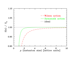
Figure 1: $S(\epsilon)/S_{0}$ versus the instanton size for the Wilson and Symanzik improved actions. The ideal action would produce a flat line at $S(\epsilon)/S_{0}=1$. The positive slope on both curves means that instantons will shrink if the Wilson or Symanzik actions are used to smooth the gauge field.

Although the Symanzik action is closer to the ideal action than the standard Wilson action, the slope is still positive for all $\rho_{inst}$ and using this action will shrink instantons.

The goal is now to select a value of $\epsilon$ that results in the flattest line possible, whilst ensuring the stability of instantons. A plot for three different values of $\epsilon$ is shown in Fig. 2.

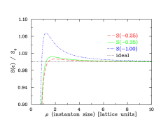
Figure 2: $S(\epsilon)$ for three different values of $\epsilon$. The larger $-\epsilon$ is made the further the curve moves from the ideal behaviour and the sharper the maximum.

With $\epsilon=-1$ the curve is similar to the mirror image of the Wilson action. For $a\rho_{inst}>1.5$, $\epsilon=-0.25$ and $-0.35$ give curves closer to the ideal, however as $|\epsilon|$ is decreased the maximum occurs at larger $\rho_{inst}$. Since it is the slope that is responsible for how an instanton’s size changes, the maximum of $S(\epsilon)$ gives the dislocation threshold of the smearing algorithm. Assuming that any topological excitation of length $\geq 2a$ is not an unphysical UV fluctuation or a lattice artifact, one should aim for a dislocation threshold of $\leq 2a$.

Given this, we propose that a value of $\epsilon=-0.25$ will be sufficient. This choice gives a dislocation threshold of $\sim\!1.97$, and a curve that is mostly flat down to values of $\rho_{inst}\sim\!1.7$. The action $S(\epsilon)/S_{0}$ is also very close to the ideal.

In Fig. 3

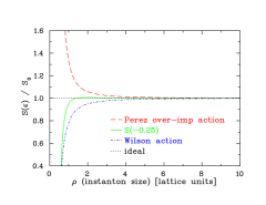
Figure 3: A comparison of $S(\epsilon)/S_{0}$ for the Perez over-improved action, our over-improved stout-link smearing $S(-0.25)$, and the standard Wilson action.

we provide a comparison of the Perez over-improved action, our over-improved action $S(-0.25)$, and the standard Wilson action. It is clear that $S(-0.25)$ should produce the best results.

Given a value for $\epsilon$ one can find a suitable value for the smearing parameter, $\rho_{sm}$. Starting from some arbitrary value, systematically increase $\rho_{sm}$ until $u_{0}$ (the mean-plaquette value) no longer increases when smearing. This value sets an upper threshold for $\rho_{sm}$ and one should then choose some $\rho_{sm}$ suitably below this threshold. In what follows we use a value of $\rho_{sm}=0.06$. A typical value for standard stout-link smearing is $\rho_{sm}\approx 0.1$. The over-improved algorithm is more sensitive to the smearing parameter than standard smearing because of the larger loops used in the smoothing procedure.

We mentioned earlier that it was the slope of $S(\epsilon)/S_{0}$ that is responsible for how an instanton will evolve under smearing. We thought it prudent to check that this was actually the case in practice by smearing a single instanton gauge field. In order to exaggerate the effects, we selected a rather extreme value of $\epsilon=-4$. A comparison of $\epsilon=-4$ and $\epsilon=-0.25$ is given in Fig. 4 . Using $\epsilon=-4$ to smear a single instanton of size $\rho_{inst}\approx 1$ should destroy the instanton. Meanwhile, if we smear an instanton with size $\rho_{inst}\approx 3.5$ it should grow rapidly when $\epsilon=-4$, and stay relatively the same size for $\epsilon=-0.25$.

Fig. 4 shows the results of the simulations.

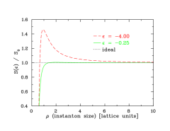
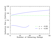
Figure 4: The evolution of a single instanton under over-improved stout-link smearing with $\epsilon=-4.0$ and $\epsilon=-0.25$. The $S(\epsilon)/S_{0}$ plots for the respective $\epsilon$ values are shown in the top plot. The bottom plot shows how an instanton of size $\rho_{inst}\approx 3.5$ grows much more rapidly with $\epsilon=-4.0$ (upper solid line) than for $\epsilon=-0.25$ (dashed curve). The lower solid curve in the bottom plot is for an instanton of size $\rho_{inst}\approx 1$ and $\epsilon=-4.0$. It has been offset by $+1.8$ to fit on the same scale as the larger instanton. We see how the instanton initially shrinks and is destroyed after 20 sweeps of over-improved stout-link smearing with $\epsilon=-4.0$.

The lowest curve is for the small instanton. Note that we offset by the size of the smaller instanton by $+1.8$ in order to display it on the same scale as the larger instanton. As expected, the small instanton initially shrinks under smearing until it is eventually destroyed in the $20^{\rm th}$ sweep. For the larger instanton we see that it does grow rapidly for $\epsilon=-4.0$, but that its size stays relatively constant for $\epsilon=-0.25$.

V Algorithm Comparisons

Given the selection of $\epsilon=-0.25$ it is now important to make a comparison of over-improved stout-link smearing with normal stout-link smearing. We are primarily concerned with the stability of the topological charge under smearing, and the structure of the gluon fields after smearing.

We use two sets of gauge fields for this study. Firstly, an ensemble of large $28\times 96$ dynamical MILC lattices Bernard et al. (2001); Aubin et al. (2004), with light quark masses; $am_{u,d}=0.0062$, $am_{s}=0.031$. We will also use a quenched MILC ensemble of the same size and lattice spacing $a=0.09$. The gauge fields were generated using a Tadpole and Symanzik improved gauge action with $1\times 1+1\times 2+1\times 1\times 1$ terms and an Asqtad staggered dynamical fermionic action for the $2+1$ flavours of dynamical quarks.

We also use some quenched CSSM gauge fields created with the ${\mathcal{O}}(a^{2})$ mean-field improved Lüscher-Weisz plaquette plus rectangle gauge action Luscher and Weisz (1985) using the plaquette measure for the mean link. The gauge-field parameters are defined by

$$\begin{split}S_{G}=&\frac{5\beta}{3}\sum_{\scriptstyle x\atop\scriptstyle\nu>\mu}\left(1-P_{\mu\nu}(x)\right)\\ &-\frac{\beta}{12\,u_{0}^{2}}\sum_{\scriptstyle x\atop\scriptstyle\nu>\mu}\left(2-R_{\mu\nu}(x)\right)\,.\end{split}$$ (26)

The plaquette measure of the tadpole improvement factor is

$$u_{0}=\left(\left\langle P_{\mu\nu}(x)\right\rangle_{x,\mu,\nu}\right)^{1/4}\,,$$ (27)

where the angular brackets indicate averaging over space-time and plaquette orientations. The CSSM configurations are generated using the Cabibbo-Marinari pseudo-heat-bath algorithm Cabibbo and Marinari (1982) using a parallel algorithm with appropriate link partitioning Bonnet et al. (2001). To improve the ergodicity of the Markov chain process, the three diagonal SU(2) subgroups of SU(3) are looped over twice Bonnet et al. (2002) and a parity transformation Leinweber et al. (2004) is applied randomly to each gauge field configuration saved during the Markov chain process.

V.1 Topological Charge

Let us first consider the evolution of the total topological charge of a gauge field under stout-link smearing. Typical studies in the past have rated a smearing algorithm’s success by its ability to generate and maintain an integer charge. We will also use this test to rate the effectiveness of the smearing procedures because of its simplicity and widespread use. However, it should be noted that we will be smoothing extremely large $28^{3}\times 96$ lattices. Due to the vast amount of non-trivial topological charge field fluctuations present it will take a lot of smoothing to generate an integer charge.

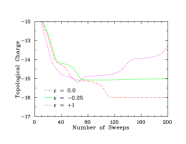
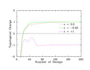
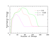
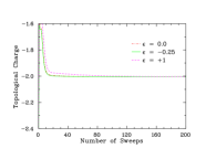
Figure 5: Plots showing how the topological charge evolves under stout link smearing when using three different actions. The top graph is for a $28\times 96$ quenched gauge field. The centre two are from an ensemble of $28\times 96$ dynamical fields with light quark masses. The bottom is a smaller $16\times 32$ quenched gauge field. The features of the graphs are explained in the main text.

Fig. 5 provides a sample of 4 different gauge fields smeared by standard, Symanzik improved, and over-improved stout-link smearing. The first is a $28^{3}\times 96$ quenched MILC gauge field, the centre two are $28^{3}\times 96$ light dynamical MILC fields, and the last is a smaller $16^{3}\times 32$ quenched field.

The top graph shows an example of the over-improved action producing a stable result. In this instance the Wilson action is fluctuating widely, and is unable to reach a stable charge within 200 sweeps of smearing. The Symanzik improved action is better in that it stabilises at around 120 sweeps, however the over-improved action is clearly superior, stabilising 50 sweeps earlier. At around 70-120 sweeps there must exist a small instanton-like object that has been removed by the errors in the Symanzik action, but preserved by the tuned over-improved action.

The second graph is a more typical example of what one sees when using the three different actions. The Wilson action is still clearly the worst of the three, fluctuating the most. Meanwhile, the Symanzik and over-improved actions are fairly similar in their behaviour. Both stabilise at the same integer charge, but the over-improved action stabilises earlier.

In the third graph we provide an example of how care must still be taken when using over-improved stout-link smearing. Contrary to the first two graphs, the curves in this graph seem to indicate that the over-improved action is the worst of the three. In this gauge field there must exist numerous instanton-like objects with size slightly greater than 1. Objects with this size will still be removed by over-improved smearing, but will survive for longer. Hence the topological charge takes longer to stabilise. The effect was great in this case because of the large lattice size, which meant it was possible for a few of these objects to exist on the lattice. The probability of finding such small objects on smaller lattices is significantly less.

The final graph is a sample of a $16^{3}\times 32$ lattice. It is shown here to demonstrate how it is much easier to smooth a smaller gauge field. Note that not all small lattices are this simple to smooth and we occasionally see behaviour similar to that in the top 3 graphs. In the larger lattices, the larger size means that there is a greater probability of finding an unstable topological object and it becomes more difficult to achieve integer charges.

V.2 Topological Charge Density

For the next part of the analysis we will directly observe the topological charge density of the gauge fields. Our aim is to directly observe the differences in the gauge fields revealed by using the Wilson and over-improved actions.

To achieve this we will require a gauge field where the final topological charges from the two smearing procedures differ. We also consider a smaller $16^{3}\times 32$ lattice because smaller lattices often provide clearer visualisations.

The topological charge, as a function of the number of smearing sweeps, is shown in Fig. 6.

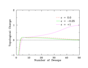
Figure 6: The topological charge evolution under smearing for a $16\times 32$ lattice. We see that when the Wilson action is used an anti-instanton is destroyed at around 20-40 sweeps. Some visualisations of the topological charge density in this region are provided later in the text.

It appears as though an anti-instanton is being destroyed by the Wilson action from about $20$ sweeps onwards. It will be interesting to visualise $q(x)$ in this region to see if we can observe this behaviour. Indeed, by considering the differences in the charge density, we were able to locate the anti-instanton that is removed by the Wilson action.

In Fig. 7 we show how the anti-instanton is affected by the Wilson action, and in Fig. 8 we have the corresponding charge density from the over-improved action.

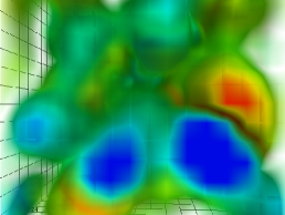
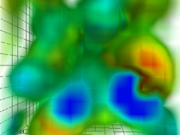
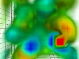
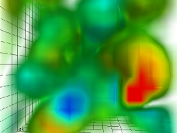
Figure 7: The evolution of the topological charge density for various sweeps of standard stout-link smearing. The sweeps shown are; 30 (top), 33, 36, 39 (bottom). In grey-scale (print) the darker areas represent regions of negative charge, and the lighter areas represent positive charge. In colour (online) blue to green represents negative topological charge and red to yellow represents positive. We see that a rather large anti-instanton is unstable under this smearing and is removed from the lattice, presenting an erroneous view of the vacuum.

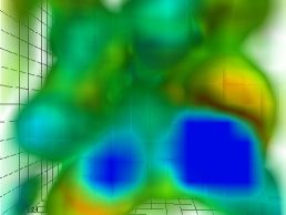
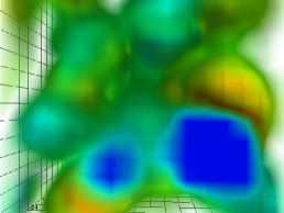
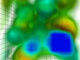
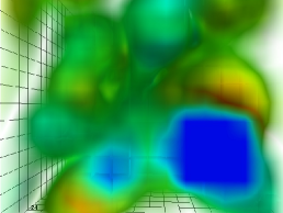
Figure 8: A visualisation of the topological charge density of the same gauge field shown in Fig. 7, this time with over-improved stout-link smearing. We see that in this case the anti-instanton in the lower right corner of the lattice is stable under smoothing, and remains stable for at least 200 sweeps.

The pictures represent a single slice of the charge density of the 4-D lattices as they evolve under the stout-link smearing. Objects with negative topological charge are coloured blue to green, and the positive objects are coloured red to yellow.

After 30 sweeps we see that both smearing methods have revealed a similar vacuum structure. The effects of the errors in the Wilson action are first seen after 33 sweeps, when the anti-instanton like object on the right begins to unwind in the upper-right corner. Here the charge density is approaching zero and therefore is not rendered. In a few sweeps the action density in this region will manifest itself in the opposite winding, largely eliminating the total topological charge. The net effect is to suggest that the instanton-like object on the right invades the neighbouring negative object. However, the change in $Q$ indicates that this is not an instanton - anti-instanton annihilation. At this point the majority of the negative topological charge density is lost and the total $Q$ for the configuration approaches $1$. This kind of phenomenon should not be seen as filtering is applied to a lattice, and indeed it does not occur when using the over-improved smearing.

After 36 sweeps the opposite winding has grown in size and it continues to grow in size as more smearing is applied to the lattice. After 39 sweeps the negatively charged object has all but disappeared. Although not shown, eventually the neighbouring positive object completely engulfs the region originally occupied by the negatively charged excitation.

This is a direct demonstration of how the discretisation errors in the Wilson action have resulted in an erroneous picture of the vacuum, and how by modifying these errors in the over-improved algorithm we are able to present a more accurate representation of the vacuum.

VI Conclusion

We have demonstrated how to define an over-improved stout-link smearing algorithm, with the aim of preserving instanton-like objects on the lattice. Using the new definition we showed how to select a suitable value of the parameter $\epsilon$, and suggest a value of $-0.25$. With the procedure defined, we demonstrated the success of the stout-link algorithm in preserving topological structures which were destroyed when using the standard Wilson action. The over-improved stout-link smearing can be used in future studies of vacuum structure or other similar applications, where preserving topology on the lattice is important.

References

- Berg (1981) B. Berg, Phys. Lett. B104, 475 (1981).
- Teper (1985) M. Teper, Phys. Lett. B162, 357 (1985).
- Ilgenfritz et al. (1986) E.-M. Ilgenfritz, M. L. Laursen, G. Schierholz, M. Muller-Preussker, and H. Schiller, Nucl. Phys. B268, 693 (1986).
- Falcioni et al. (1985) M. Falcioni, M. L. Paciello, G. Parisi, and B. Taglienti, Nucl. Phys. B251, 624 (1985).
- Albanese et al. (1987) M. Albanese et al. (APE), Phys. Lett. B192, 163 (1987).
- Bonnet et al. (2002) F. D. R. Bonnet, D. B. Leinweber, A. G. Williams, and J. M. Zanotti, Phys. Rev. D65, 114510 (2002), eprint hep-lat/0106023.
- Hasenfratz and Knechtli (2001) A. Hasenfratz and F. Knechtli, Phys. Rev. D64, 034504 (2001), eprint hep-lat/0103029.
- Morningstar and Peardon (2004) C. Morningstar and M. J. Peardon, Phys. Rev. D69, 054501 (2004), eprint hep-lat/0311018.
- Durr (2007) S. Durr (2007), eprint arXiv:0709.4110 [hep-lat].
- Symanzik (1983) K. Symanzik, Nucl. Phys. B226, 187 (1983).
- de Forcrand et al. (1996) P. de Forcrand, M. Garcia Perez, and I.-O. Stamatescu, Nucl. Phys. Proc. Suppl. 47, 777 (1996), eprint hep-lat/9509064.
- Bilson-Thompson et al. (2003) S. O. Bilson-Thompson, D. B. Leinweber, and A. G. Williams, Ann. Phys. 304, 1 (2003), eprint hep-lat/0203008.
- Garcia Perez et al. (1994) M. Garcia Perez, A. Gonzalez-Arroyo, J. Snippe, and P. van Baal, Nucl. Phys. B413, 535 (1994), eprint hep-lat/9309009.
- Bernard et al. (2001) C. W. Bernard et al., Phys. Rev. D64, 054506 (2001), eprint hep-lat/0104002.
- Aubin et al. (2004) C. Aubin et al., Phys. Rev. D70, 094505 (2004), eprint hep-lat/0402030.
- Wilson (1974) K. G. Wilson, Phys. Rev. D10, 2445 (1974).
- Bernard and DeGrand (2000) C. W. Bernard and T. A. DeGrand, Nucl. Phys. Proc. Suppl. 83, 845 (2000), eprint hep-lat/9909083.
- Belavin et al. (1975) A. A. Belavin, A. M. Polyakov, A. S. Shvarts, and Y. S. Tyupkin, Phys. Lett. B59, 85 (1975).
- Bilson-Thompson et al. (2002) S. O. Bilson-Thompson, F. D. R. Bonnet, D. B. Leinweber, and A. G. Williams, Nucl. Phys. Proc. Suppl. 109A, 116 (2002), eprint hep-lat/0112034.
- Luscher and Weisz (1985) M. Luscher and P. Weisz, Commun. Math. Phys. 97, 59 (1985).
- Cabibbo and Marinari (1982) N. Cabibbo and E. Marinari, Phys. Lett. B119, 387 (1982).
- Bonnet et al. (2001) F. D. R. Bonnet, D. B. Leinweber, and A. G. Williams, J. Comput. Phys. 170, 1 (2001), eprint hep-lat/0001017.
- Leinweber et al. (2004) D. B. Leinweber, A. G. Williams, J.-b. Zhang, and F. X. Lee, Phys. Lett. B585, 187 (2004), eprint hep-lat/0312035.