Hierarchical selection of variables in sparse high-dimensional regression

Abstract

We study a regression model with a huge number of interacting variables. We consider a specific approximation of the regression function under two assumptions: (i) there exists a sparse representation of the regression function in a suggested basis, (ii) there are no interactions outside of the set of the corresponding main effects. We suggest an hierarchical randomized search procedure for selection of variables and of their interactions. We show that given an initial estimator, an estimator with a similar prediction loss but with a smaller number of non-zero coordinates can be found.

1 Introduction

Suppose that we observe $(Y_{i},{\mathbf{X}}_{i})$, $i=1,\dots,n$, an i.i.d. sample from the joint distribution of $(Y,{\mathbf{X}})$, where $Y\in{\mathcal{R}}$, and ${\mathbf{X}}=(X_{1},\dots,X_{d})\in{\mathcal{X}}_{1}\times\cdots\times{\mathcal{X}}_{d}={\mathcal{X}}$, with ${\mathcal{X}}_{j}$ being some subsets of finite-dimensional Euclidean spaces. Our purpose is to estimate the regression function $f({\mathbf{X}})=E(Y|{\mathbf{X}})$ nonparametrically by constructing a suitable parametric approximation of this function, with data-dependent values of the parameters. We consider the situation where $n$ is large, or even very large and the dimension $d$ is also large. Without any assumptions, the problem is cursed by its dimensionality even when ${\mathcal{X}}_{j}={\mathcal{R}}$ for all $j$. For example, a histogram approximation has $p=3^{20}>10^{9}$ parameters when the number of variables is $d=20$, and the range of each is divided into the meager number of three histogram bins.

It is common now to consider models where the number of parameters $p$ is much larger than the sample size $n$. The idea is that the effective dimension is defined not by the number of potential parameters $p$ but by the (unknown) number of non-zero parameters that can be much smaller than $n$. Methods like thresholding in white noise model, cf. [Abramovich, Benjamini, Donoho and Johnstone (2006)] or [Golubev (2002)], LASSO, LARS or Dantzig selector in regression, cf, [Tibshirani (1996)], [Chen, Donoho and Saunders (2001)], [Efron, Hastie, Johnstone and Tibshirani (2004)], [Candes and Tao (2007)], are used, and it is proved that if the vector of estimated parameters is sparse (i.e., the number of non-zero parameters is relatively small) then the model can be estimated with reasonable accuracy, cf. [Bunea, Tsybakov and Wegkamp (2007a), Bunea, Tsybakov and Wegkamp (2007b), Candes and Tao (2007), Fu and Knight (2000), Greenshtein and Ritov (2004), Meinshausen and Bühlmann (2006), Meinshausen and Yu (2006), Zhang and Huang (2006), Zhao and Yu (2006)]. A direct selection of a small number of non-zero variables is relatively simple for the white noise model. There, each variable is processed separately, and the parameters can be ordered according to the likelihood that they are non-zero. The situation is more complicated in regression problems. Methods like LASSO and LARS yield numerically efficient ways to construct a sparse model, cf. [Juditsky and Nemirovski (2000), Nemirovski (2000), Osborne, Presnell and Turlach (2000b), Osborne, Presnell and Turlach (2000a), Efron, Hastie, Johnstone and Tibshirani (2004), Turlach (2005)]. However, they have their limits, and are not numerically feasible with too many parameters, as for instance in the simple example considered above.

Our aim is to propose a procedure that can work efficiently in such situations. We now outline its general scheme. Consider a collection of functions $(\psi_{i,j})_{i=1,\dots,d,\,j=0,1,\dots,L}$ where $\psi_{i,j}:{\mathcal{X}}_{i}\to{\mathcal{R}}$. For example, for fixed $i$ this can be a part of a basis $(\psi_{i,j})_{j=0,1,\dots}$ for $L_{2}({\mathcal{X}}_{i})$. For simplicity, we take the same number $L$ of basis functions for each variable. We assume that $\psi_{i,0}\equiv 1$. Consider an approximation $f_{\beta}$ of regression function $f$ given by:

$$f_{\beta}({\mathbf{X}})=\sum_{{\mathbf{j}}\in\{0,1,\dots,L\}^{d}}\beta_{{\mathbf{j}}}\prod_{i=1}^{d}\psi_{i,j_{i}}(X_{i})$$

where ${\mathbf{j}}=(j_{1},\dots,j_{d})$ and $\beta_{{\mathbf{j}}}$ are unknown coefficients. Note that $f_{\beta}$ is nothing but a specific model with interactions between variables, such that all the interactions are expressed by products of functions of a single variable. In fact, since $\psi_{i,0}\equiv 1$, the multi-indices ${\mathbf{j}}$ with only one non-zero coefficient yield all the functions of a single variable, those with only two non-zero coefficients yield all the products of two such functions, etc. Clearly, this covers the above histogram example, wavelet approximations and others.

The number of coefficients $\beta_{{\mathbf{j}}}$ in the model is $(L+1)^{d}$. The LASSO type estimator can deal with a large number of potential coefficients which grows exponentially in $n$. So, theoretically, we could throw all the factors into the LASSO algorithm and find a solution. But $p\sim L^{d}$ is typically a huge number. Although in the theory LASSO can handle that many variables, in practice, it becomes numerically infeasible. Therefore, a systematic search is needed.

Since there is no way to know in advance which factors are significant, we suggest a hierarchical selection: we build the model in a tree fashion. At each step of the iteration we apply a LASSO type algorithm to a collection of candidate functions, where we start with all functions of a single variable. Then, from the model selected by this algorithm we extract a sub-model which includes only $K$ functions, for some predefined $K$. The next step of the iteration starts with the same candidate functions as its predecessor plus all the interactions between the $K$ functions selected at the previous step.

Formally we consider the following hierarchical model selection method. For a set of functions ${\mathcal{F}}$ with cardinality $|{\mathcal{F}}|\geq K$, let ${\mathcal{M}}{\mathcal{S}}_{K}$ be some procedure to select $K$ functions out of ${\mathcal{F}}$. We denote by ${\mathcal{M}}{\mathcal{S}}_{K}({\mathcal{F}})$ the selected subset of ${\mathcal{F}}$, $|{\mathcal{M}}{\mathcal{S}}_{K}({\mathcal{F}})|=K$. Also, for a function $f:{\mathcal{X}}\to{\mathcal{R}}$, let ${\mathbb{N}}(f)$ be the minimal set of indices such that $f$ is a function of $(X_{i})_{i\in{\mathbb{N}}(f)}$ only. The procedure is defined as follows.

1. Set ${\mathcal{F}}_{0}=\cup_{i=1}^{d}\{\psi_{i,1},\dots,\psi_{i,L}\}$.

2. For $m=1,2,\dots$, let

   $${\mathcal{F}}_{m}={\mathcal{F}}_{m-1}\cup\{fg:\;f,g\in{\mathcal{M}}{\mathcal{S}}_{K}({\mathcal{F}}_{m-1}),{\mathbb{N}}(f)\cap{\mathbb{N}}(g)=\emptyset\}.$$

3. Continue until convergence is declared. The output of the algorithm is the set of functions ${\mathcal{M}}{\mathcal{S}}_{K}({\mathcal{F}}_{m})$ for some $m$.

This search procedure is valid under the dictum of no interaction outside of the set of the corresponding main effects: a term is included only if it is a function of one variable or it is a product of two other included terms. If this is not a valid assumption one can enrich the search at each step to cover all the coefficients $\beta_{{\mathbf{j}}}$ of the model. However, this would be cumbersome.

Note that $|{\mathcal{F}}_{m}|\leq K^{2}+|{\mathcal{F}}_{m-1}|\leq mK^{2}+|{\mathcal{F}}_{0}|=mK^{2}+Ld$. Thus, the set ${\mathcal{F}}_{m}$ is not excessively large. At every step of the procedure we keep for selection all the functions of a single variable, along with not too many interaction terms. In other words, functions of a single variable are treated as privileged contributors. On the contrary, interactions are considered with a suspicion increasing as their multiplicity grows: they cannot be candidates for inclusion unless their “ancestors” were included at all the previous steps.

The final number of selected effects is $K$ by construction. We should choose $K$ to be much smaller than $n$ if we want to fit our final model in the framework of the classical regression theory.

One can split the sample in two parts and do model selection and estimation separately. Theoretically, the rate of convergence of the LASSO type procedures suffers very little when the procedures are applied only to a sub-sample of the observations, as long as the sub-sample size $n_{MS}$ used for model selection is such that $n_{MS}/n$ converges slowly to 0. We can therefore, first use a sub-sample of size $n_{MS}$ to select, according to (i)–(iii), a set of $K$ terms that we include in the model. The second stage will use the rest of the sample and estimate via, e.g., standard least-square method the regression coefficients of the $K$ selected terms.

This paper has two goals. The first one, as described already, is suggesting a method to build highly complex models in a hierarchial fashion. The second purpose is arguing that a reasonable way to do model selection is a two stage procedure. The first stage can be based on the LASSO, which is an efficient way to obtain sparse representation of a regression model. We argue, however, by a way of example in Section 2 , that using solely the LASSO can be an non-optimal procedure for model selection. Therefore, in Section 3 we introduce the second stage of selection, such that a model of a desired size is obtained at the end. At this stage we suggest to use either randomized methods or the standard backward procedure. We prove prediction error bounds for two randomized methods of pruning the result of the LASSO stage. Finally, in Section 4 we consider two examples that combine the ideas presented in this paper.

2 Model selection: an example

The above hierarchical method depends on a model selection procedure ${\mathcal{M}}{\mathcal{S}}_{K}$ that we need to determine. For high-dimensional case that we are dealing with, LASSO is known to be an efficient model selection tool: it is shown that under general conditions the set of non-zero coefficients of LASSO estimator coincides with the true set of non-zero coefficients in linear regression, with probability converging to 1 as $n\to\infty$ (see, e.g., [Meinshausen and Bühlmann (2006), Zhao and Yu (2006)]). However, these results depend on strong assumptions that essentially role off anything close to multicolinearity. These conditions are often violated in practice when there are many variables representing a plentitude of highly related one to another demographic and physical measurements of the same subject. They are also violated in a common statistical learning setup where the variables of the analysis are values of different functions of one real variable (e.g., different step functions). Note that for our procedure we do not need to retain all the non-zero coefficients but just to extract the $K$ “most important” ones. To achieve this, we first tried to tune the LASSO in some natural way. However, this approach failed.

We start with an example. We use this example to argue that although the LASSO does select a small model (i.e., typically many of the coordinates of the LASSO estimator are 0), it does a poor job in selecting the relevant variables. A naive approach for model selection when the constraint applies to the number of non-zero coefficients, is to relax the LASSO algorithm until it yields a solution with the right number of variables. We believe that this is a wrong approach. The LASSO is geared for $L_{1}$ constraints and not for $L_{0}$ ones. We suggest another procedure in which we run the LASSO until it yields a model more complex than wished, but not too complex, so that a standard model selection technique like backward selection can be used. This was the method considered in [Greenshtein and Ritov (2004)] to argue that there are model selection methods which are persistent under general conditions.

We first recall the basic definition of LASSO. Consider the linear regression model

$${\mathbf{y}}={\mathbf{Z}}\beta_{0}+\varepsilon$$

where ${\mathbf{y}}=(Y_{1},\dots,Y_{n})^{\prime}\in{\mathcal{R}}^{n}$ is the vector of observed responses, ${\mathbf{Z}}\in{\mathcal{R}}^{n\times p}$ is the design matrix, $\beta_{0}\in{\mathcal{R}}^{p}$ is an unknown parameter and $\varepsilon=(\xi_{1},\dots,\xi_{n})^{\prime}\in{\mathcal{R}}^{n}$ is a noise. The LASSO estimator $\hat{}\beta_{L}$ of $\beta_{0}$ is defined as a solution of the minimization problem

$$\min_{\beta:\,\|\beta\|_{1}\leq T}\|{\mathbf{y}}-{\mathbf{Z}}\beta\|^{2}$$ (1)

where $T>0$ is a tuning parameter, $\|\beta\|_{1}$ is the $\ell_{1}$-norm of $\beta$ and $\|\cdot\|$ is the empirical norm associated to the sample of size $n$:

$$\|{\mathbf{y}}\|^{2}=n^{-1}\sum_{i=1}^{n}Y_{i}^{2}.$$

This is the formulation of the LASSO as given in [Tibshirani (1996)]. Another formulation, given below in 8 , is that of minimization of the sum of squares with $L_{1}$ penalty. Clearly, 1 is equivalent to 8 with some constant $r$ dependent on $T$ and on the data, by the Lagrange argument. The standard LARS-like algorithm of [Efron, Hastie, Johnstone and Tibshirani (2004)], which is the algorithm we used, is based on gradual relaxation of the constraint $T$ of equation 1 , and solves therefore simultaneously both problems. The focus of this paper is the selection of a model of a given size. Hence we apply the LARS algorithm until we get for the first time a model of a prescribed size.

Example 2.1

We consider a linear regression model with $100$ i.i.d. observations of $(Y,Z_{1},\dots,Z_{150})$ where the predictors $(Z_{1},\dots,Z_{150})$ are i.i.d. standard normal, the response variable is $Y=\sum_{j=1}^{150}\beta_{j}Z_{j}+\xi=\sum_{j=1}^{10}\frac{10}{25+j2}Z_{j}+\xi$, and the measurement error is $\xi\sim N(0,\sigma^{2})$, $\sigma=0.1$.

Note that we have more variables than observations but most of the $\beta_{j}$ are zero.

Figure 1 a presents the regularization path, i.e. the values of the coefficients of $\hat{}\beta_{L}$ as a function of $T$ in 1 . The vertical dashed lines indicate the values of the $T$ for which the number of non-zero coefficients of $\hat{}\beta_{L}$ is for the time larger than the mark value (multiple values of 5). The legend on the right gives the value of the 20 coefficients with the highest values (sorted by the absolute value of the coefficient).

Figure 1 b presents a similar situation. In fact, the only difference is that the correlation between any two $Z_{i}$’s is now 0.5. Again, the 10 most important variables are those with non-zero true values.

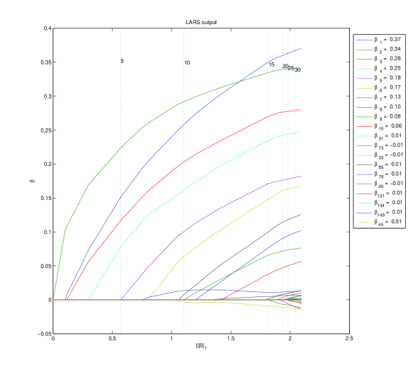
(a)

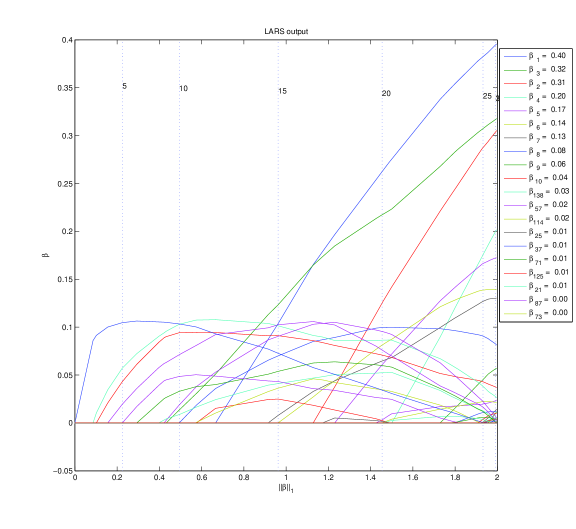
(b)

Figure 1: Selecting variables. Coefficients vs. $L_{1}$

Suppose we knew in advance that there are exactly 10 non-zero coefficients. It could be assumed that LASSO can be used, stopped when it first finds 10 non-zero coefficients (this corresponds to $T\approx 0.5$ in Figure 1 b). However, if that was the algorithm, then only three coefficients with non-zero true value, $\beta_{3}$, $\beta_{8}$, and $\beta_{10}$, were included together with some 7 unrelated variables. For $T\approx 2$ the 10 largest coefficients do correspond to the 10 relevant variables, but along with them many unrelated variables are still selected (8 variables in Figure 1 b), and moreover this particular choice of $T$ cannot be known in advance if we deal with real data.

3 Randomized selection

The approach to design the model selector ${\mathcal{M}}{\mathcal{S}}_{K}$ that we believe should be used is the one applied in the examples of Section 4 . It acts as follows: run the LASSO for a large model which is strictly larger than the model we want to consider, yet small enough so that standard methods for selecting a good subset of the variables can be implemented. Then run one of such methods, with given subset size $K$: in the examples of Section 4 we use the standard backward selection procedure. We do not have a mathematical proof which is directly relevant to such a method. We can prove, however, the validity of an inferior backward method which is based on random selection (with appropriate weights) of the variable to be dropped at each stage. We bound the increase in the sum of squares of the randomized method. The same bounds are applied necessarily to the standard backward selection.

Suppose that we have an arbitrary estimator $\tilde{}\beta$ with values in ${\mathcal{R}}^{p}$, not necessarily the LASSO estimator. We may think, for example, of any estimator of parameter $\beta_{0}$ in the linear model of Section 2 , but our argument is not restricted to that case. We now propose a randomized estimator $\widehat{}\beta$ such that:

• the prediction risk of $\widehat{}\beta$ is on the average not too far from that of $\tilde{}\beta$,

• $\widehat{}\beta$ has at most $K$ non-zero components,

• large in absolute value components of $\widehat{}\beta$ coincide with those of $\tilde{}\beta$.

Definition of the randomization distribution. Let ${\mathcal{I}}$ be the set of non-zero coordinates of the vector $\tilde{}\beta=(\tilde{}\beta_{1},\dots,\tilde{}\beta_{p})$. We suppose that its cardinality $\tilde{K}=|{\mathcal{I}}|\geq 2$. Introduce the values

$$p_{i}=\min\{1,c(\tilde{K}-1)|\tilde{}\beta_{i}|/\|\tilde{}\beta\|_{1}\},\quad i\in{\mathcal{I}},$$

where $c\geq 1$ is a solution of $\sum_{i\in{\mathcal{I}}}p_{i}=\tilde{K}-1$. Such $c$ exists since the function

$$t\mapsto\bar{p}_{i}(t)\equiv\min\{1,t(\tilde{K}-1)|\tilde{}\beta_{i}|/\|\tilde{}\beta\|_{1}\}$$

is continuous and non-decreasing, $\lim_{t\to\infty}\sum_{i\in{\mathcal{I}}}\bar{p}_{i}(t)=\tilde{K}$ and $\sum_{i\in{\mathcal{I}}}\bar{p}_{i}(1)\leq\tilde{K}-1$. From $\sum_{i\in{\mathcal{I}}}p_{i}=\tilde{K}-1$ we get

$$\sum_{i\in{\mathcal{I}}}(1-p_{i})=1,$$ (2)

so that the collection $\{1-p_{i}\}_{i\in{\mathcal{I}}}$ defines a probability distribution on ${\mathcal{I}}$ that we denote by ${\rm P}^{*}$. Note that there exists a $p_{i}$ not equal to 1 (otherwise we have $\sum_{i\in{\mathcal{I}}}p_{i}=\tilde{K}$), in particular, we have always $p_{i}<1$ for the index $i$ that corresponds to the smallest in absolute value $\tilde{}\beta_{i}$. On the other hand, $p_{i}>0$ since $\tilde{}\beta_{i}\neq 0$ for $i\in{\mathcal{I}}$. Therefore, $0<p_{i}<1$ for at least two indices $i$ corresponding to the two smallest in absolute values coordinates of $\tilde{}\beta$.

Definition of the randomized selection procedure. Choose $i^{*}$ from ${\mathcal{I}}$ at random according to distribution ${\rm P}^{*}$: ${\rm P}^{*}(i^{*}=i)=1-p_{i}$, $i\in{\mathcal{I}}$. We suppose that the random variable $i^{*}$ is independent of the data ${\bf y}$. Define a randomized estimator $\beta^{*}=(\beta^{*}_{1},\dots,\beta^{*}_{p})$ where $\beta^{*}_{i^{*}}=0$, $\beta^{*}_{i}=\tilde{}\beta_{i}/p_{i}$ for $i\in{\mathcal{I}}\setminus\{i^{*}\}$, and $\beta^{*}_{i}=0$ for $i\not\in{\mathcal{I}}$. In words, we set to zero one coordinate of $\tilde{}\beta$ chosen at random, and the other coordinates are either increased in absolute value or left intact. We will see that on the average we do not loose much in prediction quality by dropping a single coordinate in this way.

We then perform the same randomization process taking $\beta^{*}$ as initial estimator and taking randomization independently of the one used on the first step. We thus drop one more coordinate, etc. Continuing iteratively after $\tilde{K}-K$ steps we are left with the estimator which has exactly the prescribed number $K$ of non-zero coordinates. We denote this final randomized estimator by $\widehat{\beta}$. This is the one we are interested in.

Denote by ${\rm E}\mathop{\!}\nolimits^{*}$ the expectation operator with respect to the overall randomization measure which is the product of randomization measures over the $\tilde{K}-K$ iterations.

Theorem 3.1

Let ${\mathbf{Z}}\in{\mathcal{R}}^{n\times p}$ be a given matrix. Suppose that the diagonal elements of the corresponding Gram matrix ${\mathbf{Z}}^{\prime}{\mathbf{Z}}/n$ are equal to 1, and let $\tilde{}\beta$ be any estimator with $\tilde{K}\geq 3$ non-zero components. Then the randomized estimator $\widehat{}\beta$ having at most $K<\tilde{K}$ non-zero coordinates has the following properties.

• For any vector ${\bf f}\in{\mathcal{R}}^{n}$,

  $${\rm E}\mathop{\!}\nolimits^{*}\|{\bf f}-{\mathbf{Z}}\widehat{}\beta\|^{2}\leq\|{\bf f}-{\mathbf{Z}}\tilde{}\beta\|^{2}+\|\tilde{}\beta\|_{1}^{2}\left(\frac{1}{K-1}-\frac{1}{\tilde{K}-1}\right)\,.$$

• Let $\tilde{}\beta_{(j)}$ be the coordinates of $\tilde{}\beta$ ordered by absolute value: $|\tilde{}\beta_{(1)}|\geq|\tilde{}\beta_{(2)}|\geq\dots\geq|\tilde{}\beta_{(p)}|$. Suppose that $|\tilde{}\beta_{(k)}|>\|\tilde{}\beta\|_{1}/(\tilde{K}-1)$ for some $k$. Then the estimator $\widehat{}\beta$ coincides with $\tilde{}\beta$ in the $k$ largest coordinates: $\widehat{}\beta_{(j)}=\tilde{}\beta_{(j)}$, $j=1,\dots,k$.

• Suppose that $|\tilde{}\beta_{(k+1)}|=0$ and $|\tilde{}\beta_{(k)}|>\|\tilde{}\beta\|_{1}/(\tilde{K}-1)$ for some $k$. Then $\widehat{}\beta$ keeps all the non-zero coordinates of $\tilde{}\beta$.

Proof.

It is easy to see that ${\rm E}\mathop{\!}\nolimits^{*}(\beta^{*}_{i})=\tilde{}\beta_{i}$ for all $i$ and, for any vector ${\bf f}\in{\mathcal{R}}^{n}$,

$$\begin{split}\allowdisplaybreaks{\rm E}\mathop{\!}\nolimits^{*}\|{\bf f}-{\mathbf{Z}}\beta^{*}\|^{2}&=\|{\bf f}-{\mathbf{Z}}\tilde{}\beta\|^{2}+{1\over n}\mathop{\rm trace}\nolimits({\mathbf{Z}}^{\prime}{\mathbf{Z}}\Sigma^{*})\\ &=\|{\bf f}-{\mathbf{Z}}\tilde{}\beta\|^{2}+{1\over n}\sum_{i=1}^{n}{\mathbf{z}}_{i}^{\prime}\Sigma^{*}{\mathbf{z}}_{i}\\ &\leq\|{\bf f}-{\mathbf{Z}}\tilde{}\beta\|^{2}+\sum_{j=1}^{p}\tilde{}\beta_{j}^{2}\frac{1-p_{j}}{p_{j}}\end{split}$$ (3)

where ${\mathbf{z}}_{i}$ are the rows of matrix ${\mathbf{Z}}$ and $\Sigma^{*}={\rm E}\mathop{\!}\nolimits^{*}[(\beta^{*}-\tilde{}\beta)(\beta^{*}-\tilde{}\beta)^{\prime}]$ is the randomization covariance matrix. We used here that $\Sigma^{*}$ is of the form

$$\Sigma^{*}={\rm diag}\left(\tilde{}\beta_{j}^{2}\frac{1-p_{j}}{p_{j}}\right)-(B\tilde{}\beta)(B\tilde{}\beta)^{\prime}\quad\text{with}\quad B={\rm diag}\left(\frac{1-p_{i}}{p_{i}}\right),$$

and the diagonal elements of ${\mathbf{Z}}^{\prime}{\mathbf{Z}}/n$ are equal to 1, by assumption of the theorem.

Recall that $c\geq 1$, and therefore $|\tilde{}\beta_{j}|\geq\|\tilde{}\beta\|_{1}/(\tilde{K}-1)$ implies $p_{j}=1$. Hence,

$$\begin{split}\allowdisplaybreaks\sum_{j\in{\mathcal{I}}}\tilde{}\beta_{j}^{2}\frac{1-p_{j}}{p_{j}}&=\sum_{0<|\tilde{}\beta_{j}|<\|\tilde{}\beta\|_{1}/(\tilde{K}-1)}\tilde{}\beta_{j}^{2}\frac{1-p_{j}}{p_{j}}\\ &\leq\frac{\|\tilde{}\beta\|_{1}}{c(\tilde{K}-1)}\sum_{0<|\tilde{}\beta_{j}|<\|\tilde{}\beta\|_{1}/(\tilde{K}-1)}|\tilde{}\beta_{j}|(1-p_{j})\\ &\leq\frac{\|\tilde{}\beta\|_{1}^{2}}{(\tilde{K}-1)^{2}}\sum_{j\in{\mathcal{I}}}(1-p_{j})\\ &=\frac{\|\tilde{}\beta\|_{1}^{2}}{(\tilde{K}-1)^{2}}\end{split}$$ (4)

where we used 2 . Thus, the randomized estimator $\beta^{*}$ with at most $\tilde{K}-1$ non-zero components satisfies

$$\begin{split}\allowdisplaybreaks{\rm E}\mathop{\!}\nolimits^{*}\|{\mathbf{f}}-{\mathbf{Z}}\beta^{*}\|^{2}&\leq\|{\mathbf{f}}-{\mathbf{Z}}\tilde{}\beta\|^{2}+\frac{\|\tilde{}\beta\|_{1}^{2}}{(\tilde{K}-1)^{2}}\,.\end{split}$$ (5)

Note also that $\beta^{*}$ has the same $\ell_{1}$ norm as the initial estimator $\tilde{}\beta$:

$$\begin{split}\allowdisplaybreaks\|\beta^{*}\|_{1}&=\|\tilde{}\beta\|_{1}\end{split}$$ (6)

In fact, the definition of $\beta^{*}$ yields

$$\|\beta^{*}\|_{1}-\|\tilde{}\beta\|_{1} =\left(\sum_{j\in{\mathcal{I}}}\frac{|\tilde{}\beta_{j}|}{p_{j}}-\frac{|\tilde{}\beta_{i^{*}}|}{p_{i^{*}}}\right)-\sum_{j\in{\mathcal{I}}}|\tilde{}\beta_{j}|$$

$$=\frac{\|\tilde{}\beta\|_{1}}{c(\tilde{K}-1)}\sum_{p_{j}<1}\left(1-c(\tilde{K}-1)\frac{|\tilde{}\beta_{j}|}{\|\tilde{}\beta\|_{1}}\right)-\frac{\|\tilde{}\beta\|_{1}}{c(\tilde{K}-1)}$$

$$=\frac{\|\tilde{}\beta\|_{1}}{c(\tilde{K}-1)}\sum_{j\in{\mathcal{I}}}\Bigl{(}1-p_{j}\Bigr{)}-\frac{\|\tilde{}\beta\|_{1}}{c(\tilde{K}-1)}$$

$$=0,$$

in view of 2 .

Using 5 and 6 and continuing by induction we get that the final randomized estimator $\widehat{}\beta$ satisfies

$${\rm E}\mathop{\!}\nolimits^{*}\|{\mathbf{f}}-{\mathbf{Z}}\widehat{}\beta\|^{2} \leq\|{\mathbf{f}}-{\mathbf{Z}}\tilde{}\beta\|^{2}+\sum_{j=1}^{\tilde{K}-K}\frac{\|\tilde{}\beta\|_{1}^{2}}{(\tilde{K}-j)^{2}}$$

$$\leq\|{\mathbf{f}}-{\mathbf{Z}}\tilde{}\beta\|^{2}+\|\tilde{}\beta\|_{1}^{2}\left(\frac{1}{K-1}-\frac{1}{\tilde{K}-1}\right)\,.$$

This proves part (i) of the theorem. Part (ii) follows easily from the definition of our procedure, since $p_{j}=1$ for all the indices $j$ corresponding to $\tilde{}\beta_{(1)},\dots,\tilde{}\beta_{(k)}$ and the $\ell_{1}$ norm of the estimator is preserved on every step of the iterations. The same argument holds for part (iii) of the theorem. $\square$

Consider now the linear model of Section 2 . Let $\tilde{}\beta$ be an estimator of parameter $\beta_{0}$. Using Theorem 3.1 with ${\mathbf{f}}={\mathbf{Z}}\beta_{0}$ we get the following bound on the prediction loss of the randomized estimator $\widehat{}\beta$:

$$\begin{split}\allowdisplaybreaks{\rm E}\mathop{\!}\nolimits^{*}\|{\mathbf{Z}}(\widehat{}\beta-\beta_{0})\|^{2}\leq\|{\mathbf{Z}}(\tilde{}\beta-\beta_{0})\|^{2}+\|\tilde{}\beta\|_{1}^{2}\left(\frac{1}{K-1}-\frac{1}{\tilde{K}-1}\right)\,.\end{split}$$ (7)

We see that if $K$ is large enough and the norm $\|\tilde{}\beta\|_{1}^{2}$ is bounded, the difference between the losses of $\tilde{}\beta$ and $\widehat{}\beta$ is on the average not too large. For $\tilde{}\beta=\hat{}\beta_{L}$ we can replace $\|\tilde{}\beta\|_{1}^{2}$ by $T^{2}$ in 7 .

As $\tilde{}\beta$ we may also consider another LASSO type estimator which is somewhat different from $\hat{}\beta_{L}$ described in Section 2 :

$$\begin{split}\allowdisplaybreaks\tilde{}\beta=\mathop{\arg\min}_{\beta\in{\mathcal{R}}^{p}}\left\{\|{\mathbf{y}}-{\mathbf{Z}}\beta\|^{2}+r\|\beta\|_{1}\right\},\end{split}$$ (8)

where $r=A\sqrt{(\log p)/n}$ with some constant $A>0$ large enough. As shown in [Bickel, Ritov and Tsybakov (2007)], for this estimator, as well as for the associated Dantzig selector, under general conditions on the design matrix ${\mathbf{Z}}$ the $\ell_{1}$ norm satisfies $\|\tilde{}\beta\|_{1}^{2}=\|\beta_{0}\|_{1}^{2}+o_{p}(s\sqrt{(\log p)/n})$ where $s$ is the number of non-zero components of $\beta_{0}$. Thus, if $\beta_{0}$ is sparse and has a moderate $\ell_{1}$ norm, the bound 7 can be rather accurate.

Furthermore, Theorem 3.1 can be readily applied to nonparametric regression model

$${\mathbf{y}}={\mathbf{f}}+\varepsilon$$

where ${\mathbf{f}}=(f({\mathbf{X}}_{1}),\dots,f({\mathbf{X}}_{n}))^{\prime}$ and $f$ is an unknown regression function. In this case ${\mathbf{Z}}\beta=f_{\beta}({\mathbf{X}})$ is an approximation of $f({\mathbf{X}})$, for example as the one discussed in the Introduction. Then, taking as $\tilde{}\beta$ either the LASSO estimator 8 or the associated Dantzig selector we get immediately sparsity oracle inequalities for prediction loss of the corresponding randomized estimator $\widehat{}\beta$ that mimic (to within the residual term $O(\|\tilde{}\beta\|_{1}^{2}/K)$) those obtained for the LASSO in [Bunea, Tsybakov and Wegkamp (2007a), Bickel, Ritov and Tsybakov (2007)] and for the Dantzig selector in [Bickel, Ritov and Tsybakov (2007)].

It is interesting to compare our procedure with the randomization device usually referred to as the “Maurey argument”. It is implemented as a tool to prove approximation results over convex classes of functions [Barron (1993)]. Maurey’s randomization has been used in statistics in connection to convex aggregation [Nemirovski (2000)], pages 192–193 ($K$-concentrated aggregation), and [Bunea, Tsybakov and Wegkamp (2007a)], Lemma B.1.

The Maurey randomization can be also applied to our setting. Define the estimator $\widehat{}\beta_{M}$ as follows:

• choose $K<\tilde{K}$; draw independently at random $K$ coordinates from ${\mathcal{I}}$ with the probability distribution $\{|\tilde{}\beta_{i}|/\|\tilde{}\beta\|_{1}\}_{i\in{\mathcal{I}}}$,

• set the $j$th coordinate of $\widehat{}\beta_{M}$ equal to

  $$\widehat{}\beta_{Mj}=\begin{cases}\|\tilde{}\beta\|_{1}k_{j}/K&\text{ if }\tilde{}\beta_{j}>0,\\ -\|\tilde{}\beta\|_{1}k_{j}/K&\text{ if }\tilde{}\beta_{j}<0,\\ 0&\text{ if }j\not\in{\mathcal{I}}\end{cases}$$

  where $k_{j}\leq K$ is the number of times the $j$th coordinate is selected at step (i).

Note that, in general, none of the non-zero coordinates of $\widehat{}\beta_{M}$ is equal to the corresponding coordinate of the initial estimator $\tilde{}\beta$. The prediction risk of $\widehat{}\beta_{M}$ is on the average not too far from that of $\tilde{}\beta$ as the next theorem states.

Theorem 3.2

Under the assumptions of Theorem 3.1 the randomized estimator $\widehat{}\beta_{M}$ with at most $K<\tilde{K}$ non-zero coordinates satisfies

$$\begin{split}\allowdisplaybreaks{\rm E}\mathop{\!}\nolimits^{*}\|{\mathbf{f}}-{\mathbf{Z}}\widehat{}\beta_{M}\|^{2}\leq\|{\mathbf{f}}-{\mathbf{Z}}\tilde{}\beta\|^{2}+\frac{\|\tilde{}\beta\|_{1}^{2}}{K}\,.\end{split}$$ (9)

Proof.

Let $\eta_{1},\dots,\eta_{K}$ be i.i.d. random variables taking values in ${\mathcal{I}}$ with the probability distribution $\{|\tilde{}\beta_{i}|/\|\tilde{}\beta\|_{1}\}_{i\in{\mathcal{I}}}$. We have $k_{j}=\sum_{s=1}^{K}I(\eta_{s}=j)$ where $I(\cdot)$ is the indicator function. It is easy to see that ${\rm E}\mathop{\!}\nolimits^{*}(\widehat{}\beta_{Mj})=\beta_{j}$ and the randomization covariance matrix $\Sigma^{*}={\rm E}\mathop{\!}\nolimits^{*}[(\widehat{}\beta_{M}-\tilde{}\beta)(\widehat{}\beta_{M}-\tilde{}\beta)^{\prime}]$ has the form

$$\begin{split}\allowdisplaybreaks\Sigma^{*}=\frac{\|\tilde{}\beta\|_{1}}{K}{\rm diag}|\tilde{}\beta_{i}|-\frac{1}{K}|\tilde{}\beta||\tilde{}\beta|^{\prime}\end{split}$$ (10)

where $|\tilde{}\beta|$ is the vector of absolute values $|\tilde{}\beta_{i}|$. Acting as in 3 and using 10 we get

$${\rm E}\mathop{\!}\nolimits^{*}\|{\bf f}-{\mathbf{Z}}\beta_{M}\|^{2} =\|{\bf f}-{\mathbf{Z}}\tilde{}\beta\|^{2}+{1\over n}\sum_{i=1}^{n}{\mathbf{z}}_{i}^{\prime}\Sigma^{*}{\mathbf{z}}_{i}$$

$$\leq\|{\bf f}-{\mathbf{Z}}\tilde{}\beta\|^{2}+\frac{\|\tilde{}\beta\|_{1}}{K}\sum_{j\in{\mathcal{I}}}|\tilde{}\beta_{j}|$$

which yields the result. $\square$

The residual term in 9 is of the same order of magnitude $O(\|\tilde{}\beta\|_{1}^{2}/K)$ as the one that we obtained in Theorem 3.1 . In summary, $\widehat{}\beta_{M}$ does achieve the properties (A) and (B) mentioned at the beginning of this section, but not the property (C): it does not preserve the largest coefficients of $\tilde{}\beta$.

Finally, note that applying 5 with ${\mathbf{f}}={\mathbf{y}}$ we get an inequality that links the residual sums of squares (RSS) of $\beta^{*}$ and $\tilde{}\beta$:

$$\begin{split}\allowdisplaybreaks{\rm E}\mathop{\!}\nolimits^{*}\|{\mathbf{y}}-{\mathbf{Z}}\beta^{*}\|^{2}\leq\|{\mathbf{y}}-{\mathbf{Z}}\tilde{}\beta\|^{2}+\frac{\|\tilde{}\beta\|_{1}^{2}}{(\tilde{K}-1)^{2}}\,.\end{split}$$ (11)

The left hand side of 11 is bounded from below by the minimum of the RSS over all the vectors $\beta$ with exactly $\tilde{K}-1$ non-zero entries among the $\tilde{K}$ possible positions where the entries of the initial estimator $\tilde{}\beta$ are non-zero. Hence, the minimizer $\beta^{**}$ of the residual sums of squares $\|{\mathbf{y}}-{\mathbf{Z}}\beta\|^{2}$ over all such $\beta$ is an estimator whose RSS does not exceed the right hand side of 11 . Note that $\beta^{**}$ is obtained from $\tilde{}\beta$ by dropping the coordinate which has the smallest contribution to $R^{2}$. Iterating such a procedure $\tilde{K}-K$ times we get nothing but a standard backward selection. This is exactly what we apply in Section 4 . However, the estimator obtained by this non-randomized procedure has neither of the properties stated in Theorem 3.1 since we have only a control of the RSS but not necessarily of the prediction loss, and the $\ell_{1}$ norm of the estimators is not preserved from step to step, on the difference from our randomized procedure.

4 Examples

We consider here two examples of application of our method. The first one deals with simulated data.

Example 4.1

We considered a sample of size 250 from $(Y,X_{1},\dots,X_{10})$, where $X_{1},\dots,X_{10}$ are i.i.d. standard uniform, $Y=\beta_{1}\mbox{\Large$\mathbf{1}$}(\frac{1}{8}<X_{1}\leq\frac{1}{4})+\beta_{2}\mbox{\Large$\mathbf{1}$}(\frac{1}{8}<X_{2}\leq\frac{1}{2})\mbox{\Large$\mathbf{1}$}(\frac{1}{8}<X_{3}\leq\frac{3}{8})\mbox{\Large$\mathbf{1}$}(\frac{1}{8}\leq X_{4}\leq\frac{5}{8})+\varepsilon$, where $\mbox{\Large$\mathbf{1}$}(\cdot)$ denotes the indicator function and $\varepsilon$ is normal with mean 0 and variance such that the population $R^{2}$ is 0.9. The coefficients $\beta_{1}$ and $\beta_{2}$ were selected so that the standard deviation of the second term was three times that of the first.

We followed the hierarchical method (i)–(iii) of the Introduction. Our initial set ${\mathcal{F}}_{0}$ was a collection of $L=32$ step functions for each of the ten variables ($d=10$). The jump points of the step functions were equally spaced on the unit interval. The cardinality of ${\mathcal{F}}_{0}$ was 279 (after taking care of multicolinearity). At each step we run the LASSO path until $\tilde{K}=40$ variables were selected, from which we selected $K=20$ variables by the standard backward procedure. Then the model was enlarged by including interaction terms, and the iterations were continued until there was no increase in $R^{2}$.

The first step (with single effects only) ended with $R^{2}=0.4678$, and the correlation of the predicted value of $Y$ with the true one was 0.4885. The second iteration (two way interactions) ended with $R^{2}=0.6303$ and correlation with the truth of 0.6115. The third (three and four ways interactions were added) ended with $R^{2}=0.7166$ and correlation of 0.5234 with the truth. The process stopped after the fifth step. The final predictor had correlation of 0.5300 with the true predictor.

The LASSO regularization path for the final (fifth) iteration is presented in Figure 2 . The list of 20 terms included in the model is given in the legend where $i_{k}$ denotes the the $k$th step function of variable $i$. The operator $\times$ denotes interaction of variables. We can observe that the first 12 selected terms are functions of variables 1 to 4 that are in the true model. Some of the 20 terms depend also on two other variables (8 and 10) that do not belong to the true model.

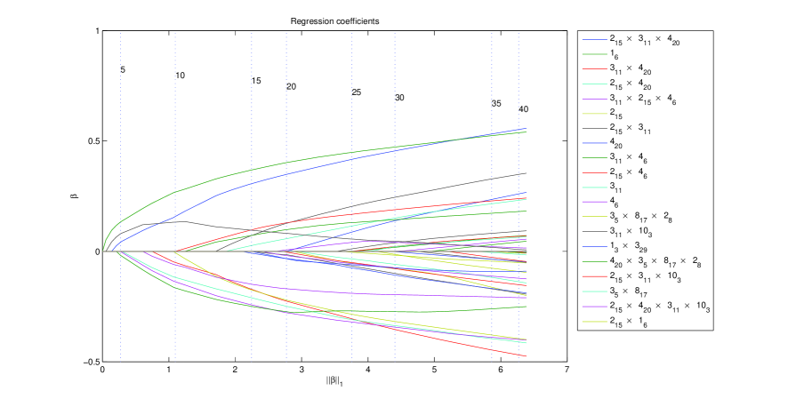
Figure 2: The final path of the LASSO algorithm for the simulation of Example 4.1 .

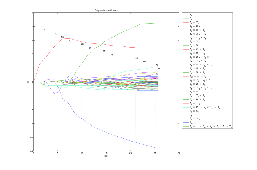
Figure 3: The final path of the LASSO algorithm for the abalone data set.

Example 4.2 (The Abalone Data)

The abalone data set, taken from ftp://ftp.ics.uci.edu/pub/machine-learning-databases/abalone/,
gives the age of abalone (as determined by cutting the shell and counting the number of rings) and some physical measurements (sex, length, diameter, height, whole weight, weight of meat, gut weight, and shell weight after being dried). The data was described initially by Nash, et al in 1994. We selected at random 3500 data points as a training set. The 677 remaining points were left as a test bed for cross-validation.

We used as a basic function of the univariate variable the ramp function $(x-a)\mbox{\Large$\mathbf{1}$}(x>a)$. The range of the variables was initially normalized to the unit interval, and we considered all break points $a$ on the grid with spacing $1/32$. However, after dropping all transformed variables which are in the linear span of those already found, we were left with only 17 variables. We applied the procedure with LASSO which ends with at most $\tilde{K}=60$ variables, from which at most $K=30$ were selected by backward regression.

The first stage of the algorithm ends with $R^{2}=0.5586$ (since we started with 17 terms and we were ready to leave up to 30 terms, nothing was gained in this stage). The second stage, with all possible main effects and two-way interactions, dealt already with 70 variables and finished with only slightly higher $R^{2}$ (0.5968). The algorithm stopped after the fifth iteration. This iteration started with 2670 terms, and ended with $R^{2}=0.5779$. The correlation of the prediction with the observed age of the test sample was 0.5051. The result of the last stage is given in Figure 3 . It can be seen that the term with the largest coefficient is that of the whole weight. Then come 3 terms involving the meat weight, and its interaction with the length. The shell weight which was most important when no interaction terms were allowed, became not important when the interactions were added.

References

- Abramovich, Benjamini, Donoho and Johnstone (2006) Abramovich, F., Benjamini, Y., Donoho, D., and Johnstone, I. (2006). Adapting to unknown sparsity by controlling the false discovery rate. Ann. Statist., 34, 584–653.
- Barron (1993) Barron, A. (1993). Universal approximation bounds for superpositions of a sigmoidal function. IEEE Transactions on Information Theory, 39, 930–945.
- Bickel, Ritov and Tsybakov (2007) Bickel, P., Ritov, Y., and Tsybakov, A. (2007). Paralleling lasso and dantzig selector. Unpublished.
- Bunea, Tsybakov and Wegkamp (2007a) Bunea, F., Tsybakov, A., and Wegkamp, M. (2007a). Aggregation for gaussian regression. Ann. Statist., 35, To be published.
- Bunea, Tsybakov and Wegkamp (2007b) Bunea, F., Tsybakov, A., and Wegkamp, M. (2007b). Sparsity oracle inequalities for the lasso. Electronic Journal of Statistics, 1, 169–194.
- Candes and Tao (2007) Candes, E. and Tao, T. (2007). The dantzig selector: statistical estimation when is much larger than . Ann. Statist., 35, To be published.
- Chen, Donoho and Saunders (2001) Chen, S., Donoho, D., and Saunders, M. (2001). Atomic decomposition by basis pursuit. SIAM Review, 43, 129–159.
- Efron, Hastie, Johnstone and Tibshirani (2004) Efron, B., Hastie, T., Johnstone, I., and Tibshirani, R. (2004). Least angle regression. Ann. Statist., 32, 407–451.
- Fu and Knight (2000) Fu, W. and Knight, K. (2000). Asymptotics for lasso-type estimators. Ann. Statist., 28, 1356–1378.
- Golubev (2002) Golubev, G. (2002). Reconstruction of sparse vectors in white gaussian noise. Problems of Information Transmission, 38, 65–79.
- Greenshtein and Ritov (2004) Greenshtein, E. and Ritov, Y. (2004). Persistency in high dimensional linear predictor-selection and the virtue of over-parametrization. Bernoulli, 10, 971–988.
- Juditsky and Nemirovski (2000) Juditsky, A. and Nemirovski, A. (2000). Functional aggregation for nonparametric estimation. Ann. Statist., 28, 681–712.
- Meinshausen and Bühlmann (2006) Meinshausen, N. and Bühlmann, P. (2006). High-dimensional graphs and variable selection with the lasso. Ann. Statist., 34, 1436–1462.
- Meinshausen and Yu (2006) Meinshausen, N. and Yu, B. (2006). Lasso type recovery of sparse representations for high dimensional data. Unpublished.
- Nemirovski (2000) Nemirovski, A. (2000). Topics in Non-parametric Statistics, Ecole d’Eté de Probabilités de Saint-Flour XXVIII - 1998, volume 1738 of Lecture Notes in Mathematics. Springer, New York.
- Osborne, Presnell and Turlach (2000a) Osborne, M., Presnell, B., and Turlach, B. (2000a). A new approach to variable selection in least squares problems. IMA Journal of Numerical Analysis, 20, 389–404.
- Osborne, Presnell and Turlach (2000b) Osborne, M., Presnell, B., and Turlach, B. (2000b). On the lasso and its dual. Journal of Computational and Graphical Statistics, 9, 319–337.
- Tibshirani (1996) Tibshirani, R. (1996). Regression shrinkage and selection via the lasso. Journal of the Royal Statistical Society, Series B., 58, 267–288.
- Turlach (2005) Turlach, B. A. (2005). On algorithms for solving least squares problems under an l1 penalty or an l1 constraint. In 2004 Proceedings of the American Statistical Association, Statistical Computing Section [CD-ROM], (pp. 2572–2577)., Alexandria, VA, 2572-2577. American Statistical Association.
- Zhang and Huang (2006) Zhang, C.-H. and Huang, J. (2006). Model-selection consistency of the lasso in high-dimensional regression. Unpublished.
- Zhao and Yu (2006) Zhao, P. and Yu, B. (2006). On model selection consistency of lasso. Journal of Machine Learning Research, 7, 2541–2563.