Collective properties of magnetobiexcitons in quantum wells’ and graphene superlattices

Abstract

We propose the Bose-Einstein condensation (BEC) and superfluidity of quasi-two-dimensional (2D) spatially indirect magnetobiexcitons in a slab of superlattice with alternating electron and hole layers consisting from the semiconducting quantum wells (QWs) and graphene superlattice in high magnetic field. The two different Hamiltonians of a dilute gas of magnetoexcitons with a dipole-dipole repulsion in superlattices consisting of both QWs and graphene layers in the limit of high magnetic field have been reduced to one effective Hamiltonian a dilute gas of two-dimensional excitons without magnetic field. Moreover, for $N$ excitons we have reduced the problem of $2N\times 2$ dimensional space onto the problem of $N\times 2$ dimensional space by integrating over the coordinates of the relative motion of an electron (e) and a hole (h). The instability of the ground state of the system of interacting two-dimensional indirect magnetoexcitons in a slab of superlattice with alternating electron and hole layers in high magnetic field is established. The stable system of indirect quasi-two-dimensional magnetobiexcitons, consisting of pair of indirect excitons with opposite dipole moments is considered. The density of superfluid component $n_{s}(T)$ and the temperature of the Kosterlitz-Thouless phase transition to the superfluid state in the system of two-dimensional indirect magnetobiexcitons, interacting as electrical quadrupoles, are obtained for both QW and graphene realizations.

PACS numbers: 71.35.Ji, 71.35.Lk, 71.35.-y, 68.65.Cd, 73.21.Cd

I Introduction

The many-particle systems of the spatially-indirect excitons in coupled quantum wells (CQWs) in the presence or absence of a magnetic field $B$ have been the subject of recent experimental investigations Snoke ; Butov ; Timofeev ; Eisenstein . These systems are of interest, in particular, in connection with the possibility of Bose-Einstein condensation (BEC) and superfluidity of indirect excitons or electron-hole pairs, which would manifest itself in the CQW as persistent electrical currents in each well and also through coherent optical properties and Josephson phenomena.Lozovik ; Birman ; Littlewood ; Vignale ; Berman In high magnetic fields, two-dimensional (2D) excitons survive in a substantially wider temperature range, as the exciton binding energies increase with magnetic field.Lerner ; Paquet ; Kallin ; Yoshioka ; Ruvinsky ; Ulloa ; Moskalenko The problem of essential interest is also collective properties of magnetoexcitons in high magnetic fields in superlattices and layered system.Filin

In this Paper we propose a new physical realization of magnetoexcitonic BEC and superfluidity in in superlattices with alternating electronic and hole layers, that is in a sense representing array of CQWs or graphene layers with spatially separated electrons ($e$) and holes $h$ with spatially separated electrons and holes in high magnetic field. Recent technological advances have allowed the production of graphene, which is a 2D honeycomb lattice of carbon atoms that form the basic planar structure in graphite Novoselov1 ; Zhang1 Graphene has been attracting a great deal of experimental and theoretical attention because of unusual properties in its band structure Novoselov2 ; Zhang2 ; Nomura ; Jain . It is a gapless semiconductor with massless electrons and holes which have been described as Dirac-fermions DasSarma . Since there is no gap between the conduction and valence bands in graphene without magnetic field, the screening effects result in the absence of excitons in graphene in the absence of magnetic field. A strong magnetic field produces a gap since the energy spectrum becomes discrete formed by Landau levels. The gap reduces screening and leads to the formation of magnetoexcitons. We also consider magnetoexcitons in the superlattices with alternating electronic and hole graphene layers. We suppose that recombination times can be much greater than relaxation times $\tau_{r}$ due to small overlapping of spatially separation of e- and h- wave functions in CQW or graphene layers. In this case electrons and holes are characterized by different quasi-equilibrium chemical potentials. Then in the system of indirect excitons in superlattices, as in CQW Lozovik ; Berman , the quasiequilibrium phases appear remark . While coupled-well structures with spatially separated electrons and holes are typically considered to be under applied electrical field, which separates electrons and holes in different quantum wellsButov ; Timofeev , we assume there are no external fields applied to a slab of superlattice. If ”electron” and ”hole” quantum wells alternate, there are excitons with parallel dipole moments in one pair of wells, but dipole moments of excitons in another neighboring pairs of neighboring wells have opposite direction. This fact leads to essential distinction of properties of $e-h$ system in superlattices from ones for coupled quantum wells with spatially separated electrons and holes (where indirect exciton system is stable due to dipole-dipole repelling of all excitons). This difference manifests itself already beginning from three-layer $e-h-e$ or $h-e-h$ system. We assume that alternating $e-h-e$ layers can be formed by independent gating with the corresponding potentials which shift chemical potentials in neighboring layers up and down or by alternating doping (by donors and acceptors, respectively).

In this Paper we reduce the problem of magnetoexcitons to the problem of excitons at $B=0$. The unstability of the ground state of the system of interacting indirect excitons in slab of superlattice with alternating $e-$ and $h-$ layers is established in strong magnetic field. Two-dimensional indirect magnetobiexcitons, consisting of the indirect magnetoexcitons with opposite dipole moments, are considered in high magnetic field. The radius and the binding energy of indirect magnetobiexciton are calculated. These magnetobiexcitons repel each other as electrical quadrupoles at long distances. In result, the system of indirect magnetobiexcitons is stable. In the ladder approximation collective spectrum of the weakly interacting by the quadrupole law two-dimensional indirect magnetobiexcitons is considered. The superfluid density $n_{s}(T)$ of interacting two-dimensional indirect magnetobiexcitons in superlattices is calculated at low temperatures $T$. We analyze the dependence of Kosterlitz-Thouless transitionKosterlitz temperature and superfluid density on magnetic field.

The rest of the Paper is organized as follows. In Sec.  II, we derive an effective Hamiltonian of magnetoexcitons in both CQWs and two graphene layers in strong magnetic field. In Sec.  III, we prove the instability of dipole magnetoexcitons in QW and graphene superlattices due to the attraction of oppositely directed dipoles. BEC and superfluidity of quadrupole magnetobiexcitons in QW and graphene superlattices has been established and analyzed in Sec.  IV. We present and discuss the numerical results in Sec.  V.

II Effective Hamiltonian of magnetoexcitons in strong magnetic field

We start with two interacting excitons in CQW in the presence of the external magnetic field $\mathbf{B}$. Without loss of generality we can take the magnetic field to be in the z direction. We find it convenient to work with the symmetric gauge for a vector potential $\mathbf{A}_{e(h)}=1/2[\mathbf{B}\times\mathbf{r}_{e(h)}]$. We employ Jacobi coordinates for the exciton center of mass $\mathbf{R}=(m_{e}\mathbf{r}_{e}+m_{h}\mathbf{r}_{h})/(m_{e}+m_{h})$ and relative motion of electrons ($e$) and holes ($h$) $\mathbf{r}=\mathbf{r}_{e}-\mathbf{r}_{h}$ and in these coordinates the Hamiltonian $\hat{H}$ for 2D spatially separated excitons is

$$\hat{H}=\int d\mathbf{R}\int d\mathbf{r}\left[\hat{\psi}^{\dagger}(\mathbf{R},\mathbf{r})\sum_{i=e,h}\left(\frac{1}{2m_{i}}\left(\mathbf{p}_{i}+\frac{e}{c}\mathbf{A}_{i}\right)^{2}\right.\right.$$ (1)

$$- \left.\left.\frac{e^{2}}{\epsilon\sqrt{(\mathbf{r}_{e}-\mathbf{r}_{h})^{2}+D^{2}}}\right)\hat{\psi}(\mathbf{R},\mathbf{r})\right]$$

$$+ \frac{1}{2}\int d\mathbf{R}_{1}\int d\mathbf{r}_{1}\int d\mathbf{R}_{2}\int d\mathbf{r}_{2}\hat{\psi}^{\dagger}(\mathbf{R}_{1},\mathbf{r}_{1})\hat{\psi}^{\dagger}(\mathbf{R}_{2},\mathbf{r}_{2})$$

$$\sum_{i,j=e,h}U^{ij}(\mathbf{r}_{i1}-\mathbf{r}_{j2})\hat{\psi}(\mathbf{R}_{2},\mathbf{r}_{2})\hat{\psi}(\mathbf{R}_{1},\mathbf{r}_{1}),$$

where $\hat{\psi}^{\dagger}(\mathbf{R},\mathbf{r})$ and $\hat{\psi}(\mathbf{R},\mathbf{r})$ are the creation and annihilation operators for magnetoexcitons; $\mathbf{r}_{e}$ and $\mathbf{r}_{h}$ are electron and hole locations along quantum wells, respectively; $D$ is the distance between electron and hole quantum wells, $e$ is the charge of an electron; $c$ is the speed of light and $\epsilon$ is a dielectric constant (for graphene layers $\epsilon$ is the dielectric constant of the matrix in which graphene layers are embedded). In Eq. (1) we use the two-particle potentials $U^{ij}$ for the electron-electron, hole-hole, electron-hole and hole-electron interaction, for electrons and holes from two different excitons: $U^{ee}(\mathbf{r}_{e1}-\mathbf{r}_{e2})=e^{2}/(\epsilon|\mathbf{r}_{e1}-\mathbf{r}_{e2}|)$, $U^{hh}(\mathbf{r}_{h1}-\mathbf{r}_{h2})=e^{2}/(\epsilon|\mathbf{r}_{h1}-\mathbf{r}_{h2}|)$, $U^{eh}(\mathbf{r}_{e1}-\mathbf{r}_{h2})=-e^{2}/(\epsilon\sqrt{|\mathbf{r}_{e1}-\mathbf{r}_{h2}|^{2}+D^{2}})$, $U^{he}(\mathbf{r}_{h1}-\mathbf{r}_{e2})=-e^{2}/(\epsilon\sqrt{|\mathbf{r}_{h1}-\mathbf{r}_{e2}|^{2}+D^{2}})$.

The four-component Hamiltonian of an isolated electron-hole pair in bilayer graphene with spatially separated electrons ($e$) and holes ($h$) in one valley in magnetic field $B$ neglecting the Coulomb interaction is given byIyengar

$$\hat{H}=v_{F}\left(\begin{array}[]{cccc}0&p_{x}^{(e)}+ip_{y}^{(e)}&0&0\\ p_{x}^{(e)}-ip_{y}^{(e)}&0&0&0\\ 0&0&0&p_{x}^{(h)}-ip_{y}^{(h)}\\ 0&0&p_{x}^{(h)}+ip_{y}^{(h)}&0\\ \end{array}\right),$$ (6)

where

$$\mathbf{p}^{(e)}=-i\hbar\nabla_{e}+\frac{e}{c}\mathbf{A}_{e};\hskip 28.45274pt\mathbf{p}^{(h)}=-i\hbar\nabla_{h}-\frac{e}{c}\mathbf{A}_{h};$$ (7)

where $e$ is an electron charge; $c$ is the speed of light; $\mathbf{r}_{e}$ and $\mathbf{r}_{h}$ are two-dimensional (2D) vectors of coordinates of an electron and hole, correspondingly; $\mathbf{A}_{e}$ and $\mathbf{A}_{h}$ are the vector potential of an electron and hole, correspondingly; $v_{F}=\sqrt{3}at/(2\hbar)$ is the Fermi velocity of electrons in graphene ($a=2.566\AA$ is the lattice constant, $t\approx 2.71eV$ is the overlap integral between the nearest carbon atoms)Lukose .

Note that the ratio of the contribution to the energy from the Zeeman term $\Delta E_{Z}(B)$ to the characteristic separation between the nearest Landau levels $\Delta E_{L}(B)$ is negligible (for quantum wells: this ratio is $\Delta E_{Z}(B)/\Delta E_{L}(B)\approx m_{e}/m_{e}^{(0)}\approx 0.1$ ; for graphene layers: at $B=10T$ this ratio is $\Delta E_{Z}(B)/\Delta E_{L}(B)\approx\mu_{B}B/(\sqrt{2}\hbar v_{F}r_{B}^{-1})\approx 5\times 10^{-3}$, where $\mu_{B}=\hbar e/(2m_{e}^{(0)}c)$ is the Bohr magneton; $m_{e}\approx 0.1m_{e}^{(0)}$ is the effective electron mass in $GaAs/AlGaAs$ quantum wells; $m_{e}^{(0)}$ is the mass of a free electron). Therefore, the contributions to the single-electron Hamiltonian from the Zeeman splitting set identically to zero analogously to Refs. [Jain, ; Iyengar, ]. We take into account the energy degeneracy corresponding to two possible spin projections in quantum wells and graphene and two graphene valleys (two pseudospins). Since electrons on a graphene lattice can be in two valleys, there are four types of excitons in bilayer graphene. Due to the fact that all these types of excitons have identical envelope wave functions and energiesIyengar , we consider below only excitons in one valley. Also, we use $n_{0}=n/(4s)$ as the density of excitons in graphene superlattice, with $n$ denoting the total density of excitons, $s$ is the spin degeneracy (equal to $4$ for magnetoexcitons in bilayer graphene). Besides, we use $n_{0}=n/s$ as the density of excitons in quantum wells, with $n$ denoting the total density of excitons, $s$ is the spin degeneracy (equal to $4$ for magnetoexcitons in coupled quantum wells).

A conserved quantity for an isolated electron-hole pair in magnetic field $B$ is the exciton generalized momentum $\hat{\mathbf{P}}$ defined as

$$\hat{\mathbf{P}}=-i\hbar\nabla_{e}-i\hbar\nabla_{h}+\frac{e}{c}(\mathbf{A}_{e}-\mathbf{A}_{h})-\frac{e}{c}[\mathbf{B}\times(\mathbf{r}_{e}-\mathbf{r}_{h})]\$$

for the Dirac equation in graphene layersIyengar as well as for the Schrödinger equation in CQWsGorkov ; Lerner ; Kallin .

The Hamiltonian of a single isolated magnetoexciton without any random field ($V_{e}(\mathbf{r}_{e})=V_{h}(\mathbf{r}_{h})=0$) is commutated with $\hat{\mathbf{P}}$, and hence they have the same the eigenfunctions, which have the following form (see Refs. [Lerner, ; Gorkov, ]):

$$\Psi_{k\mathbf{P}}(\mathbf{R},\mathbf{r})=$$

$$\exp\left\{i\mathbf{R}\left(\mathbf{P}+\frac{e}{2}\mathbf{B}\times\mathbf{R}\right)+i\gamma\frac{\mathbf{P}\mathbf{r}}{2}\right\}\Phi_{k}(\mathbf{P},\mathbf{r}),$$ (8)

where $\Phi_{k}(\mathbf{P},\mathbf{r})$ is a function of internal coordinates $\mathbf{r}$ and the eigenvalue $\mathbf{P}$ of the generalized momentum, and $k$ represents the quantum numbers of exciton internal motion. The wave function of the relative coordinate for $e$ and $h$ spatially separated in different graphene layers $\tilde{\Phi}(\mathbf{r})$ can be expressed in terms of the two-dimensional harmonic oscillator eigenfunctions $\Phi_{n_{1},n_{2}}(\mathbf{r})$. For an electron in Landau level $n_{+}$ and a hole in level $n_{-}$, the four-component wave functions for the relative coordinate areIyengar

$$\tilde{\Phi}_{n_{+},n_{-}}(\mathbf{r})=\left(\sqrt{2}\right)^{\delta_{n_{+},0}+\delta_{n_{-},0}-2}\left(\begin{array}[]{c}s_{+}s_{-}\Phi_{|n_{+}|-1,|n_{-}|-1}(\mathbf{r})\\ s_{+}\Phi_{|n_{+}|-1,|n_{-}|}(\mathbf{r})\\ s_{-}\Phi_{|n_{+}|,|n_{-}|-1}(\mathbf{r})\\ \Phi_{|n_{+}|,|n_{-}|}(\mathbf{r})\end{array}\right),$$ (13)

where $s_{\pm}=\mathrm{sgn}(n_{\pm})$. The corresponding energy of the electron-hole pair $E_{n_{+},n_{-}}^{(0)}$ (which is the eigenvalue of the Hamiltonian (Eq. (6))) is given byIyengar

$$E_{n_{+},n_{-}}^{(0)}=\frac{\hbar v_{F}}{r_{B}}\sqrt{2}\left[\mathrm{sgn}(n_{+})\sqrt{|n_{+}|}-\mathrm{sgn}(n_{-})\sqrt{|n_{-}|}\right].$$ (14)

where $r_{B}=\sqrt{c\hbar/(eB)}$ is a magnetic length; $v_{F}=\sqrt{3}at/(2\hbar)$ is the Fermi velocity of electrons in graphene ($a=2.566\AA$ is a lattice constant, $t\approx 2.71eV$ is the overlap integral between the nearest carbon atoms).Lukose The two-dimensional harmonic oscillator wave functions eigenfunctions corresponding to $e$ and $h$ in spatially separated CQWs $\Phi_{n_{1},n_{2}}(\mathbf{r})$ are given byIyengar

$$\Phi_{n_{1},n_{2}}(\mathbf{r}) = (2\pi)^{-1/2}2^{-|m|/2}\frac{\tilde{n}!}{\sqrt{n_{1}!n_{2}!}}\frac{1}{r_{B}}\mathrm{sgn}(m)^{m}\frac{r^{|m|}}{r_{B}^{|m|}}$$ (15)

$$\exp\left[-im\phi-\frac{r^{2}}{4r_{B}^{2}}\right]L_{\tilde{n}}^{|m|}\left(\frac{r^{2}}{2r_{B}^{2}}\right),$$

where $L_{\tilde{n}}^{|m|}$ denotes Laguerre polynomials; $m=n_{1}-n_{2}$; $\tilde{n}=\min(n_{1},n_{2})$, and $\mathrm{sgn}(m)^{m}\rightarrow 1$ for $m=0$. The expression for $\Phi_{k}(\mathbf{P},\mathbf{r})$ for CQW is given in Ref. [Lerner, ; Ruvinsky, ], and in Ref. [Iyengar, ]) for graphene layers. In high magnetic fields the magnetoexcitonic quantum numbers $k=\{n_{+},n_{-}\}$ for an electron in Landau level $n_{+}$ and a hole in level $n_{-}$; $\gamma=(m_{h}-m_{e})/(m_{h}+m_{e})$.

In a strong magnetic field at low densities ( $n\ll r_{B}^{-2}$ ) ($r_{B}=\sqrt{\hbar c/(eB)}$ is the magnetic length) indirect magnetoexcitons repel as parallel dipoles, and we have for the pair interaction potential:

$$\hat{U}(|\mathbf{R}_{1}-\mathbf{R}_{2}|)\equiv\hat{U}^{ee}+\hat{U}^{hh}+\hat{U}^{eh}+\hat{U}^{he}\simeq\frac{e^{2}D^{2}}{\epsilon|\mathbf{R}_{1}-\mathbf{R}_{2}|^{3}}.$$

If we expand the magnetoexciton field operators in a single magnetoexciton basis set $\Psi_{k\mathbf{P}}(\mathbf{R},\mathbf{r})$: $\hat{\psi}^{\dagger}(\mathbf{R},\mathbf{r})=\sum_{k\mathbf{P}}\Psi_{k\mathbf{P}}^{\ast}(\mathbf{R},\mathbf{r})\hat{a}_{k\mathbf{P}}^{\dagger}$; $\hat{\psi}(\mathbf{R},\mathbf{r})=\sum_{k\mathbf{P}}\Psi_{k\mathbf{P}}(\mathbf{R},\mathbf{r})\hat{a}_{k\mathbf{P}}$, where $\hat{a}_{k\mathbf{P}}^{\dagger}$ and $\hat{a}_{k\mathbf{P}}$ are the corresponding creation and annihilation operators of a magnetoexciton in $(k,\mathbf{P})$ space and substitute the expansions for the field creation and annihilation operators into the Eq. (1) and obtain the effective Hamiltonian in terms of creation and annihilation operators in $\mathbf{P}$ space. In high magnetic field, one can ignore transitions between Landau levels and consider only the lowest Landau level states (for CQWs $n_{+}=n_{-}=0$; for graphene layers $n_{+}=n_{-}=1$).

Using the orthonormality of the functions $\Phi_{k}(\mathbf{0},\mathbf{r})$ we obtain the effective Hamiltonian $\hat{H}_{\mathrm{eff}}$ in strong magnetic fields.

Due to the orthonormality of the wave functions $\Phi_{n_{+},n_{-}}(\mathbf{0,r})$ the projection of the Hamiltonian (Eq. (1)) onto the lowest Landau level results in the effective Hamiltonian, which does not reflect the spinor nature of the four-component magnetoexcitonic wave functions in graphene. Since typically, the value of $r$ is $r_{B}$, and $P\ll\hbar/r_{B}$ in this approximation, the effective Hamiltonian $\hat{H}_{\mathrm{eff}}$ in the magnetic momentum representation $P$ in the subspace the lowest Landau level (for QWs $n_{+}=n_{-}=0$; for graphene layers $n_{+}=n_{-}=1$) has the same form (compare with Ref.[Berman, ]) as for two-dimensional boson system without a magnetic field, but with the magnetoexciton magnetic mass $m_{B}$ (which depends on $B$ and $D$; see below) instead of the exciton mass ($M=m_{e}+m_{h}$), magnetic momenta instead of ordinary momenta and renormalized random field (for the lowest Landau level we denote the spectrum of the single exciton $\varepsilon_{0}(P)\equiv\varepsilon_{00}(\mathbf{P})$):

$$\hat{H}_{\mathrm{eff}}=\sum_{\mathbf{P}}\varepsilon_{0}(P)\hat{a}_{\mathbf{P}}^{\dagger}\hat{a}_{\mathbf{P}}+\frac{1}{2}$$

$$\times\sum_{\mathbf{P}_{1},\mathbf{P}_{2},\mathbf{P}_{3},\mathbf{P}_{4}}\left\langle\mathbf{P}_{1},\mathbf{P}_{2}\left|\hat{U}\right|\mathbf{P}_{3},\mathbf{P}_{4}\right\rangle\hat{a}_{\mathbf{P}_{1}}^{\dagger}\hat{a}_{\mathbf{P}_{2}}^{\dagger}\hat{a}_{\mathbf{P}_{3}}\hat{a}_{\mathbf{P}_{4}},$$ (16)

where the matrix element $\left\langle\mathbf{P}_{1},\mathbf{P}_{2}\left|\hat{U}\right|\mathbf{P}_{3},\mathbf{P}_{4}\right\rangle$ is the Fourier transform of the pair interaction potential $U(R)=e^{2}D^{2}/\epsilon R^{3}$. For an isolated magnetoexciton on the lowest Landau level at the small magnetic momenta under consideration, $\varepsilon_{0}(\mathbf{P})\approx P^{2}/(2m_{B})$, where $m_{B}$ is the effective magnetic mass of a magnetoexciton in the lowest Landau level and is a function of the distance $D$ between $e$ – and $h$ – layers and magnetic field $B$ (see Ref.[Ruvinsky, ]). In strong magnetic fields at $D\gg r_{B}$ the exciton magnetic mass is $m_{B}(D)=\epsilon D^{3}/(e^{2}r_{B}^{4})$ for QWs Ruvinsky and $m_{B}(D)=\epsilon D^{3}/(4e^{2}r_{B}^{4})$ for graphene layers Berman_Lozovik_Gumbs .

Note that the ratio of the contribution to the energy from the Zeeman term $\Delta E_{Z}(B)$ to the characteristic separation between the nearest Landau levels $\Delta E_{L}(B)$ is negligible (for quantum wells: this ratio is $\Delta E_{Z}(B)/\Delta E_{L}(B)\approx m_{e}/m_{e}^{(0)}\approx 0.1$ ; for graphene layers: at $B=10T$ this ratio is $\Delta E_{Z}(B)/\Delta E_{L}(B)\approx\mu_{B}B/(\sqrt{2}\hbar v_{F}r_{B}^{-1})\approx 5\times 10^{-3}$, where $\mu_{B}=\hbar e/(2m_{e}^{(0)}c)$ is the Bohr magneton; $m_{e}\approx 0.1m_{e}^{(0)}$ is the effective electron mass in $GaAs/AlGaAs$ quantum wells; $m_{e}^{(0)}$ is the mass of a free electron). Therefore, the contributions to the single-electron Hamiltonian from the Zeeman splitting and very small pseudospin splitting in graphene (caused by two valleys in graphene) set identically to zero analogously to Refs. [Jain, ; Iyengar, ]. We assume the energy degeneracy respect to two possible spin projections in quantum wells and graphene and two graphene valleys (two pseudospins). Since electrons on a graphene lattice can be in two valleys, there are four types of excitons in bilayer graphene. Due to the fact that all these types of excitons have identical envelope wave functions and energiesIyengar , we consider below only excitons in one valley. Also, we use $n_{0}=n/(4s)$ as the density of excitons in graphene superlattice, with $n$ denoting the total density of excitons, $s$ is the spin degeneracy (equal to $4$ for magnetoexcitons in bilayer graphene). Besides, we use $n_{0}=n/s$ as the density of excitons in quantum wells, with $n$ denoting the total density of exciton, $s$ is the spin degeneracy (equal to $4$ for magnetoexcitons in coupled quantum wells).

For large electron-hole separation $D\gg r_{B}$, transitions between Landau levels due to the Coulomb electron-hole attraction can be neglected, if the following condition is valid, (for QWs $E_{b}=e^{2}/(\epsilon_{b}D)\ll\hbar\omega_{c}=\hbar eB(m_{e}+m_{h})/(2m_{e}m_{h}c)$; for graphene layers $E_{b}=4e^{2}/(\epsilon D)\ll\hbar v_{F}/r_{B}$; where $E_{b}$ and $\omega_{c}$ are the magnetoexcitonic binding energy and the cyclotron frequency, correspondingly). This corresponds to high magnetic field $B$, large interlayer separation $D$ and large dielectric constant of the insulator layer between the graphene layers. In this notation, $v_{F}=\sqrt{3}at/(2\hbar)$ is the Fermi velocity of electrons. Also, $a=2.566\AA$ is a lattice constant, $t\approx 2.71eV$ is the overlap integral between nearest carbon atoms Lukose .

III Instability of dipole magnetoexcitons in QW and graphene superlattices

Let us show the low-density system of weakly interacting two-dimensional indirect magnetoexcitons in superlattices is instable, contrary to two-layer system in CQW. At small densities $nr_{B}^{2}\ll 1$ the system of indirect excitons at low temperatures is the two-dimensional weakly nonideal Bose gas with normal to wells dipole moments ${\bf d}$ in the ground state ($d\sim eD$, $D$ is the interwell separation), increasing with the distance between wells $D$. In contrast to ordinary excitons, for low-density spatially indirect magnetoexciton system the main contribution to the energy is originated from dipole-dipole interactions $U_{-}$ and $U_{+}$ of magnetoexcitons with opposite and parallel dipoles, respectively. Two parallel ($+$) and opposite ($-$) dipoles in low-density system interact as $U_{+}=-U_{-}=e^{2}D^{2}/\epsilon R^{3}$, where $\epsilon$ is the dielectrical constant; $R$ is the distance between dipoles along wells planes; we suppose that $D/R\ll 1$ and $L/R\ll 1$ ($L$ is the mean distance between dipoles normal to the wells). We consider the case, when the number of quantum wells $k$ in superlattice is restricted $k\ll\frac{1}{D\sqrt{\pi n}}$, and this is valid for small $k$ or for sufficiently low exciton density ($n$ is exciton surface density).

The distinction between magnetoexcitons and bosons manifests itself in exchange effects.Berman ; Snoke_book The exchange interaction in spatially separated system is suppressed in contrast to $e-h$ system in one well due to smallness of tunnel exponent $T$ connected with the penetration through barrier of dipole-dipole interaction. Hence, at $D\gg r{B}$ exchange phenomena, connected with the distinction between excitons and bosons, can be neglected for the both QWs and graphene layersBerman_Lozovik_Gumbs .

For the analysis of stability of the ground state of the weakly nonideal Bose gas of indirect excitons in superlattices we apply the Bogolubov approximation. The total Hamiltonian $\hat{H}_{tot}$ of the low-density system of indirect excitons in superlattice is given by:$\hat{H}_{tot}=\hat{H}_{0}+\hat{H}_{int}$. Here $\hat{H}_{0}$ is the effective Hamiltonian of the system of noninteracting magnetoexcitons:

$$\hat{H}_{0}=\sum_{{\bf p}}\varepsilon_{0}(p)(a_{{\bf p}}^{+}a_{{\bf p}}+b_{{\bf p}}^{+}b_{{\bf p}}+a_{-{\bf p}}^{+}a_{-{\bf p}}+b_{-{\bf p}}^{+}b_{-{\bf p}}),$$ (17)

where $\varepsilon_{0}(p)=p^{2}/(2m_{B})$ is the spectrum of isolated two-dimensional indirect magnetoexciton; $\mathbf{p}$ represents the excitonic magnetic momentum. $a_{{\bf p}}^{+}$, $a_{{\bf p}}$, $b_{{\bf p}}^{+}$, $b_{{\bf p}}$ are creation and annihilation operators of magnetoexcitons with up and down dipoles; $\hat{H}_{int}$ is the effective Hamiltonian of the interaction between magnetoexcitons:

$$\begin{array}[]{c}\hat{H}_{int}=\frac{U}{2S}\sum_{{\bf p}_{1}+{\bf p}_{2}={\bf p}_{3}+{\bf p}_{4}}(a_{{\bf p}_{4}}^{+}a_{{\bf p}_{3}}^{+}a_{{\bf p}_{2}}a_{{\bf p}_{1}}+\\ b_{{\bf p}_{4}}^{+}b_{{\bf p}_{3}}^{+}b_{{\bf p}_{2}}b_{{\bf p}_{1}}-a_{{\bf p}_{4}}^{+}a_{{\bf p}_{3}}^{+}b_{{\bf p}_{2}}b_{{\bf p}_{1}}-b_{{\bf p}_{4}}^{+}b_{{\bf p}_{3}}^{+}a_{{\bf p}_{2}}a_{{\bf p}_{1}}-\\ a_{{\bf p}_{4}}^{+}b_{{\bf p}_{3}}^{+}a_{{\bf p}_{2}}b_{{\bf p}_{1}}),\end{array}$$

$S$ is the surface of the system. Let us consider the temperature $T=0$. Assuming the majority of particles are in the condensate ($N-N_{0}/N_{0}\ll 1$, where $N$ and $N_{0}$ are the total number of particles and the number of particles in condensate), we account as in Bogolubov approximation only interaction between condensate particles and excited particles with condensate particles, neglecting by the interaction between noncondensate particles. Then the total Hamiltonian transforms to:

$$\begin{array}[]{c}\hat{H}_{tot}=\frac{1}{2}\sum_{{\bf p}\neq 0}[\varepsilon_{0}(p)(a_{{\bf p}}^{+}a_{{\bf p}}+b_{{\bf p}}^{+}b_{{\bf p}}+a_{-{\bf p}}^{+}a_{-{\bf p}}+\\ b_{-{\bf p}}^{+}b_{-{\bf p}})-Un(a_{{\bf p}}^{+}b_{-{\bf p}}^{+}+a_{{\bf p}}b_{-{\bf p}}+a_{-{\bf p}}^{+}b_{{\bf p}}^{+}+a_{-{\bf p}}b_{{\bf p}}\\ +a_{{\bf p}}^{+}b_{{\bf p}}+a_{-{\bf p}}^{+}b_{-{\bf p}}+a_{{\bf p}}b_{{\bf p}}^{+}+a_{-{\bf p}}b_{-{\bf p}}^{+})],\end{array}$$

In Eq.(III) terms, arising from first and second terms of the Hamiltonian Eq.(III), which describe the repulsion of the indirect magnetoexcitons with parallel dipole moments, are compensating by other terms of the Hamiltonian Eq.(III), describing the attraction of indirect magnetoexcitons with opposite dipoles. In the result only terms describing the attraction survive. Let us diagonalize Hamiltonian $\hat{H}_{tot}$ by using of the unitary transformation of the Bogolubov typeAbrikosov

$$\begin{array}[]{c}a_{\bf p}=\frac{1}{\sqrt{1-A_{{\bf p}}^{2}-B_{{\bf p}}^{2}}}(\alpha_{\bf p}+A_{\bf p}\alpha_{-{\bf p}}^{+}+B_{\bf p}\beta_{-{\bf p}}^{+});\\ b_{\bf p}=\frac{1}{\sqrt{1-A_{{\bf p}}^{2}-B_{{\bf p}}^{2}}}(\beta_{\bf p}+A_{\bf p}\beta_{-{\bf p}}^{+}+B_{\bf p}\alpha_{-{\bf p}}^{+}),\end{array}$$

where the coefficients $A_{\bf p}$ and $B_{\bf p}$ are found from the condition of vanishing of coefficients at nondiagonal terms in Hamiltonian. In result we obtain

$$\hat{H}_{tot}=\sum_{{\bf p}\neq 0}\varepsilon(p)(\alpha_{{\bf p}}^{+}\alpha_{{\bf p}}+\beta_{{\bf p}}^{+}\beta_{{\bf p}})$$ (18)

with the spectrum of quasiparticles $\varepsilon(p)$:

$$\varepsilon(p)=\sqrt{(\varepsilon_{0}(p))^{2}-(nU)^{2}}.$$ (19)

At small momenta $p<\sqrt{2m_{B}nU}$ the spectrum of excitations becomes imaginary. Hence, the system of weakly interacting indirect magnetoexcitons in slab of superlattice is unstable. It can be seen that the condition of the instability of magnetoexcitons as stronger as magnetic field higher, because $m_{B}$ increases with the increase of magnetic field, and, therefore, the region of $p$ resulting in the imaginary collective spectrum increases as $B$ increases.

This, on first view, strange result can be illustrated by the following example. There are equal number of dipoles oriented up and down. Let us consider four dipoles, two of them being oriented up and two — down. It is easy to count that number of repelling pairs is smaller than that of attracting ones. The prevailing of attraction leads to unstability.

IV BEC and superfluidity of quadrupole magnetobiexcitons in QW and graphene superlattices

Let us consider as the ground state of the system the low-density weakly nonideal gas of two-dimensional indirect magnetobiexcitons, created by indirect magnetoexcitons with opposite dipoles in neighboring pairs of wells (Fig. 1). The small parameter at the adiabatic approximation is the numerical small parameter which is equal to the ratio of magnetobiexciton and magnetoexciton energies or the ratio between radii of magnetoexciton and magnetobiexciton along quantum wells (or graphene layers) (see, e.g., Ref. [Musin, ]). These parameters are small, and they are even smaller than analogous parameters for atoms and molecules. The smallness of these parameters will be verified below by the results of the calculation of indirect magnetobiexciton. Here it was assumed, that the distance between wells (or graphene layers) $D$ is greater than the radius of indirect magnetobiexciton $a_{b}$. The potential energy of interaction between indirect magnetoexcitons with opposite dipoles $U(r)$ has the form shown on Fig. 2 ($r$ is the distance between indirect magnetoexcitons along quantum wells/graphene layers):

$$U(r)=\frac{e^{2}}{\epsilon r}-\frac{2e^{2}}{\epsilon\sqrt{r^{2}+D^{2}}}+\frac{e^{2}}{\epsilon\sqrt{r^{2}+4D^{2}}}.$$ (20)

At $r>1.11D$ indirect magnetoexcitons attract, and at $r<1.11D$ they repel. The minimum of potential energy $U(r)$ locates at $r=r_{0}\approx 1.67D$ between indirect excitons. At large $D$ one can expand the potential energy $U(r)$ on the parameter $r-r_{0}/D\ll 1$:

$$U(r)=-0.04\frac{e^{2}}{\epsilon D}+0.44\frac{e^{2}}{\epsilon D^{3}}(r-r_{0})^{2}.$$ (21)

So at large $D$ magnetobiexciton levels correspond to the two-dimensional harmonic oscillator with the frequency $\omega=0.88e^{2}/(m_{B}\epsilon D^{3})$:

$$E_{n}=-0.04\frac{e^{2}}{\epsilon D}+2\sqrt{2}E_{0}\left(\frac{r^{*}}{D}\right)^{3/2}(n+1),$$ (22)

where $E_{0}=m_{B}e^{\prime 4}/(\hbar^{2}\epsilon)$, $r^{*}=\hbar^{2}\epsilon/(2m_{B}e^{\prime 2})$, $e^{\prime 2}=0.88e^{2}$. In the ground state the characteristic spread of magnetobiexciton $a_{b}$ along quantum wells/graphene layers (near the mean radius of magnetobiexciton $r_{0}$ along wells/graphene layers) is:

$$a_{b}=\sqrt{\frac{2\hbar}{m_{B}\omega}}=(8r^{*})^{1/4}D^{3/4}=1.03a_{ex},$$ (23)

where $a_{ex}=(8r^{ex})^{1/4}D^{3/4}$; $r^{ex}=\hbar^{2}\epsilon/(2m_{B}e^{2})$ is the two-dimensional effective Bohr radius with the effective magnetic mass $m_{B}$. Hence, the ratio of the binding energies of magnetobiexciton and magnetoexciton is: $E_{bex}/E_{ex}=0.04\ll 1$ at $D\gg a_{ex}$ (the ratio of radii of magnetoexciton and magnetobiexciton is $r_{0}/a_{ex}=0.67(8r^{ex})^{1/4}D^{-1/4}\ll 1$). So adiabatic condition is valid.

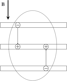
Figure 1: Two-dimensional indirect magnetobiexcitons consisting of indirect magnetoexcitons with opposite dipole moments, located in neighboring pairs of wells/graphene layers.

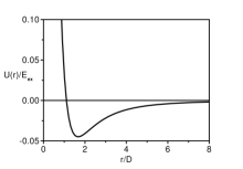
Figure 2: The potential energy $U(r)$ of the interaction of indirect magnetoexcitons with opposite dipoles, located in neighboring pairs of wells or graphene layers (in units of the binding energy of indirect magnetoexciton $E_{ex}=e^{2}/\epsilon D$), as a function of the distances $r$ between magnetoexcitons along the wells/graphene layers (in units of $D$).

The mean dipole moment of indirect magnetobiexciton is equal to zero. However, the quadrupole moment is nonzero and equal to $Q=3eD^{2}$ (the large axis of the quadrupole is normal to quantum wells/graphene layers). So indirect magnetobiexcitons interact at long distances $R\gg D$ as parallel quadrupoles: $U(R)=9e^{2}D^{4}/(\epsilon R^{5})$.

Exchange effects, connected with the distinction between low-density indirect magnetobiexcitons and bosons, can be suppressed due to the negligible overlapping of wave functions of two magnetobiexcitons on account of the potential barrier, associated with the quadrupole repulsion of indirect magnetobiexcitons at long distances analogously to dipole magnetoexcitons. At large $D$ the small tunnelling parameter connected with this barrier has the form $exp[-0.93\sqrt{D/r^{ex}}]$. Hence, at $D\gg r^{ex}$ exchange effects for indirect magnetobiexcitons can be neglected.

We account the scattering of magnetobiexciton on magnetobiexciton by using of the results of the theory of two-dimensional Bose-gas.Lozovik The chemical potential $\mu$ of two-dimensional biexcitons, repulsed by the quadrupole law, in the ladder approximation, has the form (compare to Refs. [Lozovik, ; Berman, ]):

$$\mu=\frac{4\pi\hbar^{2}n_{bex}}{m_{B}^{b}\log\left[\hbar^{4/3}\epsilon^{2/3}/\left(8\pi(9m_{B}^{b}e^{2}D^{4})^{2/3}n_{bex}\right)\right]}.$$ (24)

where $n_{bex}=n/(2s)$ is the density of magnetobiexcitons in QWs and $n_{bex}=n/(8s)$ in graphene layers; $m_{B}^{b}=2m_{B}$ is the mass of a magnetobiexciton.

At small momenta the collective spectrum of magnetobiexciton system is the sound-like $\varepsilon(p)=c_{s}p$ ($c_{s}=\sqrt{\mu/m_{B}^{b}}$ is the sound velocity) and satisfied to Landau criterion for superfluidity. The density of the superfluid component $n_{S}(T)$ for two-dimensional system with the sound spectrum can be estimated as:Griffin

$$n_{S}(T)=n_{bex}-\frac{3\zeta(3)}{2\pi\hbar^{2}}\frac{k_{B}^{3}T^{3}}{m_{B}^{b}c_{s}^{4}}.$$ (25)

The second term in Eq.(25) is the temperature dependent normal density taking into account gas of phonons (”bogolons”) with dispersion law $\varepsilon(p)=\sqrt{\mu/m_{B}^{b}}p$, $\mu$ is given by Eq.(24).

In a 2D system, superfluidity of magnetobiexcitons appears below the Kosterlitz-Thouless transition temperature $T_{c}=\pi n_{S}(T)/(2m_{B}^{b})$, where only coupled vortices are present Kosterlitz . Employing $n_{S}(T)$ for the superfluid component, we obtain an equation for the Kosterlitz-Thouless transition temperature $T_{c}$ with solution

$$T_{c}=\left[\left(1+\sqrt{\frac{32}{27}\left(\frac{m_{B}^{b}k_{B}T_{c}^{0}}{\pi\hbar^{2}n_{bex}}\right)^{3}+1}\right)^{1/3}\right.$$

$$-\left.\left(\sqrt{\frac{32}{27}\left(\frac{4m_{B}^{b}k_{B}T_{c}^{0}}{\pi\hbar^{2}n_{bex}}\right)^{3}+1}-1\right)^{1/3}\right]\frac{T_{c}^{0}}{2^{1/3}}\ .$$ (26)

Here, $T_{c}^{0}$ is an auxiliary quantity, equal to the temperature at which the superfluid density vanishes in the mean-field approximation, i.e., $n_{S}(T_{c}^{0})=0$, $T_{c}^{0}=k_{B}^{-1}\left(2\pi\hbar^{2}nc_{s}^{4}m_{B}^{b}/(3\zeta(3))\right)^{1/3}$. The temperature $T_{c}^{0}=T_{c}^{0}(B,D)$ may be used to estimate the crossover region where local superfluid density appears for magnetobiexcitons on a scale smaller or of the order of the mean intervortex separation in the system. The local superfluid density can manifest itself in local optical or transport properties. The dependence of $T_{c}$ on the density of magnetoexcitons at different magnetic field $B$ for superlattice consisting of quantum wells and graphene layers is represented on Fig. 3.

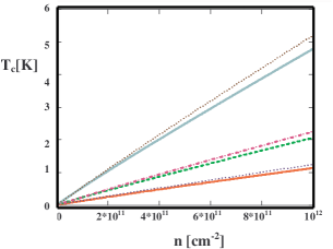
Figure 3: Dependence of temperature of Kosterlitz-Thouless transition $T_{c}=T_{c}(B)$ (in units $K$) for the superlattice consisting of quantum wells (for $GaAs/AlGaAs$: $\epsilon=13$); and (for graphene layers separated by the layer of $SiO_{2}$: $\epsilon=4.5$) on the magnetoexciton density $n$ (in units $cm^{-2}$) at the interlayer separation $D=10nm$ at different magnetic fields $B$: $B=20T$ – solid curve for quantum wells and dotted curve for graphene layers; $B=15T$ – dashed curve for quantum wells and dashed-dotted curve for graphene layers; $B=10T$ – thin solid curve for quantum wells and solid and thin dotted curve for graphene layers.

V Discussion

It is shown that the low-density system of indirect magnetoexcitons in a slab of superlattice consisting of alternating $e$ and $h$ in QWs or GLs in high magnetic field occur to be instable due to the attraction of magnetoexcitons with opposite dipoles at large distances. Note that in spite of both QW and graphene realizations are represented by completely different Hamiltonians, the effective Hamiltonian in a strong magnetic field was obtained to be the same. Moreover, for $N$ excitons we have reduced the number of the degrees of freedom from $2N\times 2$ to $N\times 2$ by integrating over the coordinates of the relative motion of e and h. The instability of the ground state of the system of interacting two-dimensional indirect magnetoexcitons in a slab of superlattice with alternating electron and hole layers of both QWs and GLs in high magnetic field is claimed due to the attraction between the indirect excitons with opposite directed dipole moments. The stable system occurs to be indirect quasi-two-dimensional magnetobiexcitons, consisting from indirect excitons with opposite directed dipole moments. The stability of the system is connected with the quadrupole-quadrupole repulsion of indirect magnetoexcitons. So at the pumping increase at low temperatures the excitonic line must vanish and only magnetobiexcitonic line survives. The Kosterlitz-Thouless transition to the superfluid state is calculated for the system of indirect magnetobiexcitons. According to Eq. (26), the temperature $T_{c}$ for the onset of superfluidity due to the Kosterlitz-Thouless transition at a fixed magnetobiexciton density decreases as a function of magnetic field $B$ and interlayer separation $D$. This is due to the increased effective magnetic mass $m_{B}$ of magnetoexcitons as a functions of $B$ and $D$. The $T_{c}$ decreases as $B^{-{1}/{2}}$ at $D\ll r_{B}$ or as $B^{-2}$ when $D\gg r_{B}$. According to Fig. 3, the Kosterlitz-Thouless temperature $T_{c}$ is higher for the superlattice consisting of graphene layers than for the superlattice consisting of the quantum wells, and this difference is as stronger as the magnetic field is smaller.

- (1) D. W. Snoke, Science 298, 1368 (2002).
- (2) L. V. Butov, J. Phys.: Condens. Matter 16, R1577 (2004).
- (3) V. B. Timofeev and A. V. Gorbunov, J. Appl. Phys. 101, 081708 (2007).
- (4) J. P. Eisenstein and A. H. MacDonald, Nature 432, 691 (2004).
- (5) Yu. E. Lozovik and V. I. Yudson, JETP Lett. 22, 26(1975); JETP 44, 389 (1976); Physica A 93, 493 (1978).
- (6) J. Zang, D. Schmeltzer and J. L. Birman, Phys. Rev. Lett. 71, 773 (1993).
- (7) X. Zhu, P. Littlewood, M. Hybertsen and T. Rice, Phys. Rev. Lett. 74, 1633 (1995).
- (8) G. Vignale and A. H. MacDonald, Phys. Rev. Lett. 76 2786 (1996).
- (9) Yu. E. Lozovik and O. L. Berman, JETP Lett. 64, 573 (1996); JETP 84, 1027 (1997).
- (10) I. V. Lerner and Yu. E. Lozovik, JETP 51, 588 (1980); JETP, 53, 763 (1981); A. B. Dzyubenko and Yu. E. Lozovik, J. Phys. A 24, 415 (1991).
- (11) D. Paquet, T. M. Rice, and K. Ueda, Phys. Rev. B32, 5208 (1985).
- (12) C. Kallin and B. I. Halperin, Phys. Rev. B30, 5655 (1984); Phys. Rev. B31, 3635 (1985).
- (13) D. Yoshioka and A. H. MacDonald, J. Phys. Soc. Jpn 59, 4211 (1990).
- (14) Yu. E. Lozovik and A. M. Ruvinsky, Phys. Lett. A 227, 271 (1997); JETP 85, 979 (1997).
- (15) M. A. Olivares-Robles and S. E. Ulloa, Phys. Rev. B64, 115302 (2001).
- (16) S. A. Moskalenko, M. A. Liberman, D. W. Snoke and V. V. Botan, Phys. Rev. B66, 245316 (2002).
- (17) A. I. Filin, V. B. Timofeev, S. I. Gubarev, D. Birkedal and J. M. Hvam, JETP Lett. 65, 623 (1997); A. V. Larionov, V. B. Timofeev, P. A. Ni, S. V. Dubonos, J. Hvam, and K. Soerensen, JETP Lett. 75 570 (2002).
- (18) K. S. Novoselov et al., Science 306, 666 (2004).
- (19) Y. Zhang, J. P. Small, M. E. S. Amori and P. Kim, Phys. Rev. Lett. 94, 176803 (2005).
- (20) K. S. Novoselov et al., Nature (London) 438, 197 (2005).
- (21) Y. B. Zhang et al., Nature (London) 438, 201 (2005).
- (22) K. Nomura and A. H. MacDonald, Phys. Rev. Lett. 96, 256602 (2006).
- (23) C. Tőke, P. E. Lammert, V. H. Crespi, and J. K. Jain, Phys. Rev. B74, 235417 (2006).
- (24) S. Das Sarma, E. H. Hwang, and W.- K. Tse, Phys. Rev. B75, 121406(R) (2007).
- (25) These phases are analogous to these for layered equilibrium system with equal chemical potentials for electrons and holes.
- (26) J. M. Kosterlitz and D. J. Thouless, J. Phys. C 6, 1181 (1973); D. R. Nelson and J. M. Kosterlitz, Phys. Rev. Lett. 39, 1201 (1977).
- (27) A. Iyengar, J. Wang, H. A. Fertig, and L. Brey, Phys. Rev. B75, 125430 (2007).
- (28) V. Lukose, R. Shankar, and G. Baskaran, Phys. Rev. Lett. 98, 116802 (2007).
- (29) L. P. Gorkov and I. E. Dzyaloshinskii, JETP 26, 449 (1967).
- (30) O. L. Berman, Yu. E. Lozovik, and G. Gumbs, Phys. Rev. Lett. submitted (2007); (cond-mat/0706.0244).
- (31) S. A. Moskalenko and D. W. Snoke, Bose-Einstein Condensation of Excitons and Biexcitons and Coherent Nonlinear Optics with Excitons (Cambridge University Press, New-York 2000).
- (32) A. A. Abrikosov, L. P. Gorkov, and I. E. Dzyaloshinskii, Methods of Quantum Field Theory in Statistical Physics, (Prentice-Hall, Englewood Cliffs, N.J., 1963).
- (33) L. N. Ivanov, Yu. E. Lozovik, and D. R. Musin, J. Phys. C 11, 2527 (1978).
- (34) A. Griffin, Excitations in a Bose-Condensed Liquid (Cambridge University Press, Cambridge, England, 1993).