The chemical enrichment of the ICM from hydrodynamical simulations

Abstract

The study of the metal enrichment of the intra–cluster and inter–galactic media (ICM and IGM) represents a direct means to reconstruct the past history of star formation, the role of feedback processes and the gas–dynamical processes which determine the evolution of the cosmic baryons. In this paper we review the approaches that have been followed so far to model the enrichment of the ICM in a cosmological context. While our presentation will be focused on the role played by hydrodynamical simulations, we will also discuss other approaches based on semi–analytical models of galaxy formation, also critically discussing pros and cons of the different methods. We will first review the concept of the model of chemical evolution to be implemented in any chemo–dynamical description. We will emphasise how the predictions of this model critically depend on the choice of the stellar initial mass function, on the stellar life–times and on the stellar yields. We will then overview the comparisons presented so far between X–ray observations of the ICM enrichment and model predictions. We will show how the most recent chemo–dynamical models are able to capture the basic features of the observed metal content of the ICM and its evolution. We will conclude by highlighting the open questions in this study and the direction of improvements for cosmological chemo–dynamical models of the next generation.

1 Introduction

Clusters of galaxies are the ideal cosmological signposts to trace the past history of the inter–galactic medium (IGM), thanks to the high density and temperature reached by the cosmic baryons trapped in their gravitational potential wells (Rosati et al. 2002; Voit 2005; Diaferio et al. 2008 - Chapter 2, this volume). Observations in the X–ray band with the Chandra and XMM–Newton satellites are providing invaluable information on the thermodynamical properties of the intra–cluster medium (ICM) (Kaastra et al. 2008 - Chapter 9, this volume). These observations highlight that non–gravitational sources of energy, such as energy feedback from supernovae (SNe) and Active Galactic Nuclei (AGN) have played an important role in determining the ICM physical properties. Spatially resolved X–ray spectroscopy permits to measure the equivalent width of emission lines associated to transitions of heavily ionised elements and, therefore, to trace the pattern of chemical enrichment (e.g., Mushotzky 2004 for a review). In turn, this information is inextricably linked to the history of formation and evolution of the galaxy population (e.g., Renzini 1997 and references therein), as inferred from observations in the optical/near-IR band. For instance, De Grandi et al. (2004) have first shown that cool core clusters are characterised by a significant central enhancement of the iron abundance, which closely correlates with the magnitude of the Brightest Cluster Galaxies (BCGs). This demonstrates that a fully coherent description of the evolution of cosmic baryons in the condensed stellar phase and in the diffuse hot phase requires properly accounting for the mechanisms of production and release of both energy and metals.

The study of how these processes take place during the hierarchical build up of cosmic structures has been tackled with different approaches. Semi–analytical models (SAMs) of galaxy formation provide a flexible tool to explore the space of parameters which describe a number of dynamical and astrophysical processes. In their most recent formulation, such models are coupled to dark matter (DM) cosmological simulations, to trace the merging history of the halos where galaxy formation takes place, and include a treatment of metal production from type-Ia and type-II supernovae (SN Ia and SN II, hereafter; De Lucia et al. 2004; Nagashima et al. 2005), so as to properly address the study of the chemical enrichment of the ICM. The main limitation of this method is that it does not include the gas dynamical processes which causes metals, once produced, to be transported in the ICM. As a consequence, they provide a description of the global metallicity of clusters and its evolution, but not of the details of its spatial distribution.

In order to overcome this limitation, Cora (2006) applied an alternative approach, in which non–radiative hydrodynamical simulations of galaxy clusters are used to trace at the same time the formation history of DM halos and the dynamics of the gas. In this approach, metals are produced by SAM galaxies and then suitably assigned to gas particles, thereby providing a chemo–dynamical description of the ICM. Domainko et al. (2006) used hydrodynamical simulations, which include prescriptions for gas cooling, star formation and feedback, similar to those applied in SAMs, to address the specific role played by ram–pressure stripping to distribute metals, while Kapferer et al. (2007b) used the same approach to study the different roles played by galactic winds and by ram–pressure stripping. While these approaches offer advantages with respect to standard SAMs, they still do not provide a fully self–consistent picture, in which chemical enrichment is the outcome of the process of star formation, associated to the cooling of the gas infalling in high density regions. In this sense, a fully self–consistent approach requires that the simulations include the processes of gas cooling, star formation and evolution, along with the corresponding feedback in energy and metals.

A number of authors have presented hydrodynamical simulations for the formation of cosmic structures, which include treatments of the chemical evolution at different levels of complexity. Raiteri et al. (1996) presented SPH simulations of the Galaxy, forming in an isolated halo, by following iron and oxygen production from SN II and SN Ia, also accounting for the effect of stellar lifetimes. Mosconi et al. (2001) performed a detailed analysis of chemo–dynamical SPH simulations, aimed at studying both numerical stability of the results and the enrichment properties of galactic objects in a cosmological context. Lia et al. (2002) discussed a statistical approach to follow metal production in SPH simulations, which have a large number of star particles, showing applications to simulations of a disc–like galaxy and of a galaxy cluster. Kawata & Gibson (2003b) carried out cosmological chemo–dynamical simulations of elliptical galaxies, with an SPH code, by including the contribution from SN Ia and SN II, also accounting for stellar lifetimes. Valdarnini (2003) performed an extended set of cluster simulations and showed that profiles of the iron abundance are steeper than the observed ones. A similar analysis has been presented by Romeo et al. (2006), who also considered the effect of varying the IMF and the feedback efficiency on the enrichment pattern of the ICM. Scannapieco et al. (2005) presented an implementation of a model of chemical enrichment in the GADGET-2 code, coupled to a self–consistent model for star formation and feedback. In their model, which was applied to study the enrichment of galaxies, they included the contribution from SN Ia and SN II, assuming that all long–lived stars die after a fixed delay time. Tornatore et al. (2007a, 2004) presented results from an implementation of a detailed model of chemical evolution model in the GADGET-2 code (Springel 2005), including metallicity–dependent yields and the contribution from intermediate and low mass stars (ILMS hereafter). The major advantage of this approach is that the metal production is self–consistently predicted from the rate of gas cooling treated by the hydrodynamical simulations, without resorting to any external model. However, at present the physical scales involved by the processes of star formation and SN explosions are far from being resolved in simulations which sample cosmological scales. For this reason, such simulations also need to resort to external sub–resolution models, which provide an effective description of a number of relevant astrophysical processes.

The aim of this paper is to provide a review of the results obtained so far in the study of the chemical enrichment of the ICM in a cosmological context. Although we will concentrate the discussion on the results obtained from full hydrodynamical simulations, we will also present results based on SAMs. As such, this paper complements the reviews by Borgani et al. 2008 - Chapter 13, this volume, which reviews the current status in the study of the thermodynamical properties of the ICM with cosmological hydrodynamical simulations, and by Schindler & Diaferio 2008 - Chapter 17, this volume, which will focus on the study of the role played by different physical processes in determining the ICM enrichment pattern. Also, this paper will not present a detailed description of the techniques for simulations of galaxy clusters, which is reviewed by Dolag et al. 2008 - Chapter 12, this volume.

In Sect. 2 we review the concept of model of chemical evolution and highlight the main quantities which are required to fully specify this model. In Sect. 3 we review the results on the global metal content of the ICM, while Sect. 4 concentrates on the study of the metallicity profiles and Sect. 5 on the study of the ICM evolution. Sect. 6 discusses the properties of the galaxy population. Finally, Sect. 7 provides a critical summary of the results presented, by highlighting the open problems and lines of developments to be followed by simulations of the next generation.

2 What is a model of chemical evolution?

In this section we provide a basic description of the key ingredients required by a model of chemical evolution. For a more detailed description we refer to the book by Matteucci (2003).

The process of star formation in cosmological hydrodynamical simulations is described through the conversion of a gas element into a star particle; as a consequence, in simulations of large volumes the star particles have a mass far larger than that of a single star, with values of the order of $10^{6}$–$10^{8}$ M_⊙, depending on the resolution and on the mass of the simulated structure (e.g., Katz et al. 1996). The consequence of this coarse–grained representation of star formation is that each star particle must be treated as a simple stellar population (SSP), i.e. as an ensemble of coeval stars having the same initial metallicity. Every star particle carries all the physical information (e.g. birth time $t_{\mathrm{b}}$, initial metallicity and mass) that is needed to calculate the evolution of the stellar populations that they represent, once the lifetime function (see Sect. 2.2), the IMF (see Sect. 2.4) and the yields (see Sect. 2.3) for SNe and ILMS have been specified. Therefore, we can compute for every star particle at any given time $t>t_{\mathrm{b}}$ how many stars are dying as SN II and SN Ia, and how many stars undergo the AGB phase, according to the equations of chemical evolution, that we will present here below.

The generation of star particles is pertinent to hydrodynamical simulations, which include the description of the star formation. As for semi–analytic models (SAMs) of galaxy formation, they generally identify a galaxy with a suitably chosen DM particle in the collisionless simulation which is used to reconstruct the merger tree. While this DM particle defines the position of a galaxy, the corresponding stellar content is described as a superposition of SSPs, each generated in correspondence of the time step with which the process of galaxy formation is studied (e.g., Diaferio et al. 2001; De Lucia et al. 2004; Nagashima et al. 2005, for applications of SAMs to the cluster galaxies). In this sense, the description of the chemical evolution model, as we provide here, can be used for both hydrodynamical simulations and for SAMs.

It is generally assumed that the stars having mass above $8$ M_⊙ at the end of the hydrostatic core burning undergo an electron capture process, leading to a core collapse. A large amount of energy can be transferred to the outer layers during this phase due to a substantial production of neutrinos that easily escape from the central core. Although theoretical work has not yet been able to reproduce a sufficient energy deposition, it is currently supposed that this process leads to an explosive ejection of the outer layers, giving rise to a SN II. We remind the reader that $8$ M_⊙ is a commonly adopted fiducial value, although the limiting mass for the onset of explosive evolution is still debated (e.g., Portinari et al. 1998).

A different ejection channel is provided by the SN Ia that are believed to arise from thermonuclear explosions of white dwarfs (WD hereafter) in binary stellar systems as a consequence of the matter accretion from the companion (e.g., Nomoto et al. 2000). However, there are still a number of uncertainties about the nature of both the WD and the companion and about the mass reached at the onset of the explosion (e.g., Matteucci & Recchi 2001, Yungelson & Livio 2000). Furthermore, observational evidences for multiple populations of Type Ia progenitors have been recently found both from direct detection of Type Ia events (e.g., Mannucci et al. 2005, Scannapieco & Bildsten 2005, Sullivan et al. 2006) or from inferences on the chemical enrichment patterns in galaxy clusters (e.g., Gal-Yam & Maoz 2004). Finally, a third way to eject heavy elements in the interstellar medium is the mass loss of ILMS by stellar winds.

In summary, the main ingredients that define a model of chemical evolution are the following: (a) the SNe explosion rates, (b) the adopted lifetime function, (c) the adopted yields and (d) the IMF which fixes the number of stars of a given mass. We describe each of these ingredients in the following.

2.1 The equations of chemical evolution

2.1.1 Type Ia supernovae

We provide here below a short description of how Type Ia SN are included in a model of chemical evolution. For a comprehensive review of analytical formulations we refer to the paper by Greggio (2005). Following Greggio & Renzini (1983), we assume here that SN Ia arise from stars belonging to binary systems, having mass in the range 0.8–8 M_⊙. Accordingly, in the single–degenerate WD scenario (Nomoto et al. 2000), the rate of explosions of SN Ia can be written as

$$R_{{\mathrm{SN\,Ia}}}(t)\,=\,A\,\int\limits_{\displaystyle{M_{\mathrm{B,inf}}}}^{\displaystyle{M_{\mathrm{B,sup}}}}\phi(m_{\mathrm{B}})\int\limits_{\displaystyle{\mu_{\mathrm{m}}}}^{\displaystyle{\mu_{\mathrm{M}}}}f(\mu)\,\psi(t-\tau_{m_{2}})\,{\mathrm{d}}\mu\,{\mathrm{d}}m_{\mathrm{B}}\,.$$ (1)

In the above equation, $\phi(m)$ is the IMF, $m_{\mathrm{B}}$ is the total mass of the binary system, $m_{2}$ is the mass of the secondary companion, $\tau_{m}$ is the mass–dependent life–time and $\psi(t)$ is the star formation rate. The variable $\mu=m_{2}/m_{\mathrm{B}}$ is distributed according to the function $f(\mu)$, while $A$ is the fraction of stars in binary systems of that particular type to be progenitors of SN Ia (see Matteucci & Recchi 2001 for more details). For instance, in the model by Greggio & Renzini (1983) $\mu$ varies in the range between $\mu_{\mathrm{m}}$ and $\mu_{\mathrm{M}}=0.5$, with $\mu_{\mathrm{m}}=\max\left[m_{2}(t)/m_{\mathrm{B}},(m_{\mathrm{B}}-0.5M_{\mathrm{BM}})/m_{\mathrm{B}}\right]$, where $m_{2}(t)$ is the mass of the companion which dies at the time $t$, according to the chosen life-time function. Furthermore, let $M_{\mathrm{Bm}}$ and $M_{\mathrm{BM}}$ be the smallest and largest value allowed for the progenitor binary mass $m_{\mathrm{B}}$. Then, the integral over $m_{\mathrm{B}}$ runs in the range between $M_{\mathrm{B,inf}}$ and $M_{\mathrm{B,sup}}$, which represent the minimum and the maximum value of the total mass of the binary system that is allowed to explode at the time $t$. These values in general are functions of $M_{\mathrm{Bm}}$, $M_{\mathrm{BM}}$, and $m_{2}(t)$, which in turn depends on the star formation history $\Psi(t)$. The exact functional dependence is defined by the SN Ia progenitor model. For instance, in the model by Greggio & Renzini (1983) it is $M_{\mathrm{B,inf}}=\max[2m_{2}(t),M_{\mathrm{Bm}}]$ and $M_{\mathrm{B,sup}}=0.5M_{\mathrm{BM}}+m_{2}(t)$. Under the assumption of a short duration burst of star formation, the function $\psi(t)$ can be approximated with a Dirac $\delta$–function. This case applies to hydrodynamical simulations, which include star formation, where the creation of a SSP is described by an impulsive star formation event, while more complex descriptions should take into account the continuous star formation history $\psi(t)$. Under the above assumption for $\psi(t)$ and using the functional form of $f(\mu)$ derived from statistical studies of the stellar population in the solar neighbourhood (Tutukov & Iungelson 1980; Matteucci & Recchi 2001), we find

$$R_{\mathrm{SN\,Ia}}(t)\,=\,-{{\mathrm{d}}m_{2}(t)\over{\mathrm{d}}t}\bigg{|}_{m_{2}\equiv\tau^{-1}(t)}24\,m_{2}^{2}\,A\int_{M_{\mathrm{Bm}}}^{M_{\mathrm{BM}}}\phi(m_{\mathrm{B}})\frac{1}{m_{\mathrm{B}}^{3}}{\mathrm{d}}m_{\mathrm{B}}\,.$$ (2)

Since the current understanding of the process of star formation does not allow to precisely determine the value of $A$, its choice can be fixed from the requirement of reproducing a specific observation, once the form of the IMF is fixed. For instance, Matteucci & Gibson (1995) found that $A=0.1$ was required to reproduce the observed iron enrichment.

2.1.2 Supernova Type II and low and intermediate mass stars

Computing the rates of SN II and ILMS is conceptually simpler, since they are driven by the lifetime function $\tau(m)$ convolved with the star formation history $\psi(t)$ and multiplied by the IMF $\phi(m=\tau^{-1}(t))$. Again, since $\psi(t)$ is a delta–function for the SSP used in simulations, the SN II and ILMS rates read

$$R_{{\mathrm{S}N\,II}|{\mathrm{I}LMS}}(t)=\phi(m(t))\times\left(-\frac{{\mathrm{d}}\,m(t)}{{\mathrm{d}}\,t}\right)$$ (3)

where $m(t)$ is the mass of the star that dies at time $t$. We note that the above expression must be multiplied by a factor of $(1-A)$ for AGB rates if the interested mass $m(t)$ falls in the same range of masses which is relevant for the secondary stars of SN Ia binary systems.

In order to compute the metal release by stars (binary systems in case of SN Ia) of a given mass we need to take into account the yields $p_{Z_{i}}(m,Z)$, which provide the mass of the element $i$ produced by a star of mass $m$ and initial metallicity $Z$. Then, the equation which describes the evolution of the mass $\rho_{i}(t)$ for the element $i$, holding for a generic form of the star formation history $\psi(t)$, reads:

$$\begin{array}[]{lcl}\dot{\rho}_{i}(t)&=&-\psi(t)Z_{i}(t)\\ &\\ &+&A\int\limits_{M_{\mathrm{Bm}}}^{M_{\mathrm{BM}}}\phi(m)\left[\int\limits_{\mu_{\min}}^{0.5}f(\mu)\psi(t-\tau_{m_{2}})p_{Z_{i}}(m,Z)\,{\mathrm{d}}\mu\right]\,{\mathrm{d}}m\\ &\\ &+&(1-A)\int\limits_{M_{\mathrm{Bm}}}^{M_{\mathrm{BM}}}\psi(t-\tau(m))p_{Z_{i}}(m,Z)\varphi(m)\,{\mathrm{d}}m\\ &\\ &+&\int\limits_{M_{\mathrm{L}}}^{M_{\mathrm{Bm}}}\psi(t-\tau(m))p_{Z_{i}}(m,Z)\varphi(m)\,{\mathrm{d}}m\\ &\\ &+&\int\limits_{M_{\mathrm{BM}}}^{M_{\mathrm{U}}}\psi(t-\tau(m))p_{Z_{i}}(m,Z)\varphi(m)\,{\mathrm{d}}m.\end{array}$$ (4)

In the above equation, $M_{\mathrm{L}}$ and $M_{\mathrm{U}}$ are the minimum and maximum mass of a star, respectively. Commonly adopted choices for these limiting masses are $M_{\mathrm{L}}\simeq 0.1$ M_⊙ and $M_{\mathrm{U}}\simeq 100$ M_⊙. The term in the first line of Eq. 4 accounts for the metallicity sink due to the locking of metals in the newborn stars. The term in the second line accounts for metal ejection contributed by SN Ia. The terms in the third and fourth lines describe the enrichment by mass–loss from intermediate and low mass stars, while the last line accounts for ejecta by SN II.

2.2 The lifetime function

Different choices for the mass–dependence of the life–time function have been proposed in the literature. For instance, Padovani & Matteucci (1993) (PM93 hereafter) proposed the expression

$$\tau(m)=\left\{\begin{array}[]{ll}10^{[(1.34-\sqrt{1.79-0.22(7.76-\log(m))})/0.11]-9}\,\,\,{\rm for}\,\,m\leq 6.6~{}{\rm M}_{\odot}\\ \\ 1.2\,m^{-1.85}+0.003\,\,\,\,\,{\rm otherwise.}\\ \end{array}\right.$$ (5)

An alternative expression has been proposed by Maeder & Meynet (1989) (MM89 hereafter), and extrapolated by Chiappini et al. (1997) to very high ($>60$ M_⊙) and very low ($<1.3$ M_⊙) masses:

$$\tau(m)=\left\{\begin{array}[]{ll}10^{-0.6545\log m+1}&m\leq 1.3~{}{\rm M}_{\odot}\\ \vspace{-0.2cm}&\\ 10^{-3.7\log m+1.351}&1.3<m\leq 3~{}{\rm M}_{\odot}\\ \vspace{-0.2cm}&\\ 10^{-2.51\log m+0.77}&3<m\leq 7~{}{\rm M}_{\odot}\\ \vspace{-0.2cm}&\\ 10^{-1.78\log m+0.17}&7<m\leq 15~{}{\rm M}_{\odot}\\ \vspace{-0.2cm}&\\ 10^{-0.86\log m-0.94}&15<m\leq 53~{}{\rm M}_{\odot}\\ \vspace{-0.3cm}&\\ 1.2\times m^{-1.85}+0.003&{\rm otherwise.}\end{array}\right.$$ (6)

The main difference between these two functions concerns the life–time of low mass stars ($<8\,$M_⊙). The MM89 life–time function delays the explosion of stars with mass $\gtrsim 1~{}$M_⊙, while it anticipates the explosion of stars below $1~{}$M_⊙ with respect to the PM93 life–time function. Only for masses below $1$ M_⊙ does the PM93 function predict much more long–living stars. This implies that different life–times will produce different evolution of both absolute and relative abundances (we refer to Romano et al. (2005) for a detailed description of the effect of the lifetime function in models of chemical evolution).

We point out that the above lifetime functions are independent of metallicity, whereas in principle this dependence can be included in a model of chemical evolution (e.g., Portinari et al. 1998). For instance, Raiteri et al. (1996) used the metallicity–dependent lifetimes as obtained from the Padova evolutionary tracks (Bertelli et al. 1994). We show in Fig. 1 a comparison of different lifetime functions.

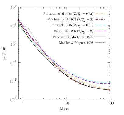
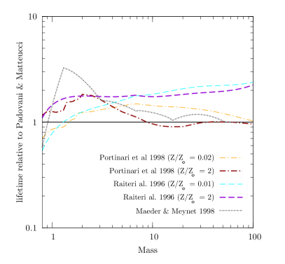
Figure 1: Left panel: the mass dependence of different lifetime functions: Padovani & Matteucci (1993, solid line), Maeder & Meynet (1998, dotted line), Raiteri et al. (1996, dashed lines; the thin line refers to $Z=0.02\,Z_{\odot}$, the thick line refers to $Z=2\,Z_{\odot}$), Portinari et al. (1998, dot–dashed lines; the thin line refers to $Z=0.02\,Z_{\odot}$, the thick line refers to $Z=2\,Z_{\odot}$). Right panel: the ratio between the same lifetimes and that by Padovani & Matteucci (1993).

2.3 Stellar yields

The stellar yields specify the quantity $p_{Z_{i}}(m,Z)$, which appears in Eq. 4 and, therefore, the amount of different metal species which are released during the evolution of a SSP. A number of different sets of yields have been proposed in the literature, such as those by Renzini & Voli (1981), van den Hoek & Groenewegen (1997), Marigo (2001) for the LIMS and those by Nomoto et al. (1997), Iwamoto et al. (1999), Thielemann et al. (2003) for SN Ia. As for SN II, there are many proposed sets of metallicity–dependent yields; among others, those by Woosley & Weaver (1995), by Portinari et al. (1998), by Chieffi & Limongi (2004), which are based on different assumptions of the underlying model of stellar structure and evolution.

As an example of the differences among different sets of yields, we show in the left panel of Fig. 2 the ratios between the abundances of different elements produced by the SN II of a SSP, as expected from Woosley & Weaver (1995) and from Chieffi & Limongi (2004). Different curves and symbols here correspond to different values of the initial metallicity of the SSP. Quite apparently, the two sets of yields provide significantly different metal masses, by an amount which can sensitively change with initial metallicity. This illustrates how a substantial uncertainty exists nowadays about the amount of metals produced by different stellar populations. There is no doubt that these differences between different sets of yields represent one of the main uncertainties in any modelling of the chemical evolution of the ICM.

For this reason, we recommend that papers related to the cosmological modelling of the chemical evolution, either by SAMs or by hydrodynamical simulations, should be very careful in specifying for which set of yields the computations have been performed as well as the details of assumed lifetime and models for SN II and SN Ia. In the absence of this, it becomes quite hard to judge the reliability of any detailed comparison with observational data or with the predictions of other models.

2.4 The initial mass function

The initial mass function (IMF) is one of the most important quantities in a model of chemical evolution. It directly determines the relative ratio between SN II and SN Ia and, therefore, the relative abundance of $\alpha$–elements and Fe–peak elements. The shape of the IMF also determines how many long–living stars will form with respect to massive short–living stars. In turn, this ratio affects the amount of energy released by SNe and the present luminosity of galaxies, which is dominated by low mass stars, and the (metal) mass–locking in the stellar phase.

As of today, no general consensus has been reached on whether the IMF at a given time is universal or strongly dependent on the environment, or whether it is time–dependent, i.e. whether local variations of the values of temperature, pressure and metallicity in star–forming regions affect the mass distribution of stars.

The IMF $\phi(m)$ is defined as the number of stars of a given mass per unit logarithmic mass interval. A widely used form is

$$\phi(m)\,=\,dN/d\log m\propto m^{-x(m)}\,.$$ (7)

If the exponent $x$ in the above expression does not depend on the mass $m$, the IMF is then described by a single power–law. The most famous and widely used single power–law IMF is the Salpeter (1955) one that has $x=1.35$. Arimoto & Yoshii (1987, AY hereafter) proposed an IMF with $x=0.95$, which predicts a relatively larger number of massive stars. In general, IMFs providing a large number of massive stars are usually called top–heavy. More recently, different expressions of the IMF have been proposed in order to model a flattening in the low–mass regime that is currently favoured by a number of observations. Kroupa (2001) introduced a multi–slope IMF, which is defined as

$$\phi(m)\,\propto\,\left\{\begin{array}[]{ll}m^{-1.3}&\qquad m\geq 0.5\,{\rm M}_{\odot}\\ \vspace{-0.2cm}&\\ m^{-0.3}&\qquad 0.08\leq m<0.5\,{\rm M}_{\odot}\\ \vspace{-0.2cm}&\\ m^{\ 0.7}&\qquad m\leq 0.08\,{\rm M}_{\odot}\\ \end{array}\right.$$ (8)

Chabrier (2003) proposed another expression for the IMF, which is quite similar to that one proposed by Kroupa

$$\phi(m)\,\propto\,\left\{\begin{array}[]{ll}m^{-1.3}&\qquad m>1\,{\rm M}_{\odot}\\ \vspace{-0.2cm}&\\ e^{\frac{-\left(\log(m)-\log(m_{c})\right)^{2}}{2\,\sigma^{2}}}&\qquad m\leq 1\,{\rm M}_{\odot}\\ \end{array}\right.$$ (9)

Theoretical arguments (e.g. Larson 1998) suggest that the present–day characteristic mass scale, where the IMF changes its slope, $\sim 1$ M_⊙ should have been larger in the past, so that the IMF at higher redshift was top–heavier than at present.

While the shape of the IMF is determined by the local conditions of the inter–stellar medium, direct hydrodynamical simulations of star formation in molecular clouds are only now approaching the required resolution and sophistication level to make credible predictions on the IMF (e.g., Bonnell et al. 2006, Padoan et al. 2007; see McKee & Ostriker 2007 for a detailed discussion).

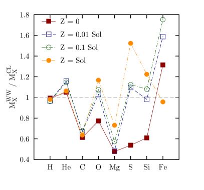
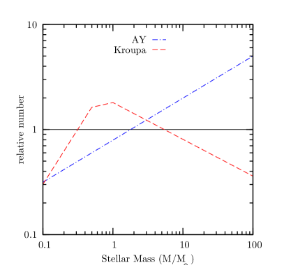
Figure 2: Left panel: the ratio $M_{j}^{\mathrm{WW}}/M_{j}^{\mathrm{CL}}$ between the mass of species $j$, produced by the SN II of a SSP, when using the two sets of yields by Woosley & Weaver (1995) and by Chieffi & Limongi (2004) for different values of the initial SSP metallicity. Different symbols are for different values of the initial metallicity of the SSP, as reported by the labels. From Tornatore et al. (2007a). Right panel: the shape of different IMFs introduced in the literature. Stellar masses are expressed in units of M_⊙.

We show in Fig. 2 the number of stars, as a function of their mass, predicted by different IMFs, relative to those of the Salpeter IMF. As expected, the AY IMF predicts a larger number of high–mass stars and, correspondingly, a smaller number of low–mass stars, the crossover taking place at $\simeq 2$ M_⊙. As a result, we expect that the enrichment pattern of the AY IMF will be characterised by a higher abundance of those elements, like oxygen, which are mostly produced by SN II. Both the Kroupa and the Chabrier IMFs are characterised by a relative deficit of very low–mass stars and a mild overabundance of massive stars and ILMS. Correspondingly, an enhanced enrichment in both Fe–peak and $\alpha$ elements like oxygen is expected, mostly due to the lower fraction of mass locked in ever–living stars. For reference we also show a different IMF, also proposed by Kroupa et al. (1993), that exhibits a deficit in both very low– and high–mass stars; for this kind of IMF a lower $\alpha\,/\,$Fe ratio with respect to the Salpeter IMF is expected.

Since clusters of galaxies basically behave like “closed boxes”, the overall level of enrichment and the relative abundances should directly reflect the condition of star formation. While a number of studies have been performed so far to infer the IMF shape from the enrichment pattern of the ICM, no general consensus has been reached. For instance, Renzini (1997, 2004) and Pipino et al. (2002) argued that both the global level of ICM enrichment and the $\alpha$/Fe relative abundance can be reproduced by assuming a Salpeter IMF, as long as this relative abundance is sub-solar. Indeed, a different conclusion has been reached by other authors in the attempt of explaining the relative abundances $[\alpha/{\rm Fe}]\,\raise-2.0pt\hbox{\hbox to0.0pt{\hbox{$\sim$}\hss}\raise 5.0pt\hbox{$>$}\ }0$ in the ICM (e.g., Baumgartner et al. 2005). Portinari et al. (2004) used a phenomenological model to argue that a standard Salpeter IMF cannot account for the observed $\alpha$/Fe ratio in the ICM. As we shall discuss in the following, a similar conclusion was also reached by Nagashima et al. (2005), who used semi–analytical models of galaxy formation to trace the production of heavy elements, and by Romeo et al. (2005), who used hydrodynamical simulations including chemical enrichment. Saro et al. (2006) analysed the galaxy population from simulations of galaxy clusters and concluded that a Salpeter IMF produces a colour–magnitude relation that, with the exception of the BCGs, is in reasonable agreement with observations. On the contrary, the stronger enrichment provided by a top–heavier IMF turns into too red galaxy colours.

In the following sections, the above results on the cosmological modelling of the ICM will be reviewed in more detailed, also critically discussing the possible presence of observational biases, which may alter the determination of relative abundances and, therefore, the inference of the IMF shape.

Different variants of the chemical evolution model have been implemented by different authors in their simulation codes. For instance, the above described model of chemical evolution has been implemented with minimal variants by Kawata & Gibson (2003a), Kobayashi (2004), who also included the effect of hypernova explosions, and Tornatore et al. (2007a), while Tornatore et al. (2007b) also included the effect of metal enrichment from low–metallicity (Pop III) stars. Raiteri et al. (1996) and Valdarnini (2003) also used a similar model, but neglected the contribution from low- and intermediate-mass stars. Mosconi et al. (2001) and Scannapieco et al. (2005) neglected delay times for SN II, assumed a fixed delay time for SN Ia and neglected the contribution to enrichment from low- and intermediate-mass stars.

Clearly, a delicate point in hydrodynamical simulations is deciding how metals are distributed to the gas surrounding the star particles. The physical mechanisms actually responsible for enriching the inter–stellar medium (ISM; e.g., stellar winds, blast waves from SN explosions, etc.) take place on scales which are generally well below the resolution of current cosmological simulations of galaxy clusters (see Schindler & Diaferio 2008 - Chapter 17, this volume). For this reason, the usually adopted procedure is that of distributing metals according to the same kernel which is used for the computation of the hydrodynamical forces, a choice which is anyway quite arbitrary. Mosconi et al. (2001) and Tornatore et al. (2007a) have tested the effect of changing in different ways the weighting scheme to distribute metals and found that final results on the metal distribution are generally rather stable. Although this result is somewhat reassuring, it is clear that this warning on the details of metal distribution should always be kept in mind, at least until our simulations will have enough resolution and accurate description of the physical processes determining the ISM enrichment (Schindler & Diaferio 2008 - Chapter 17, this volume).

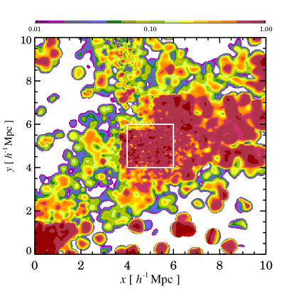
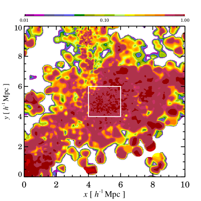
Figure 3: Maps of the fractional contribution of SN II to the global metallicity (from Tornatore et al. 2007a). The left panel refer to the Salpeter IMF, while the right panel is for the AY top–heavy IMF. The white square is centred on the minimum of the cluster gravitational potential and its size is about twice the value of $R_{200}$.

Figure 4: Iron mass ejection rate as a function of redshift for SN Ia (top panel) and SN II (bottom panel), as predicted by the semi–analytical model by Cora (2006). The thick solid line is for the products released by the BCG, while the other curves are for galaxies lying within different cluster-centric distances, as computed at $z=0$, after excluding the BCG contribution.

3 Global abundances

As a first step in our overview of the results of the ICM enrichment, we discuss a few general features of the enrichment pattern, which are related to the underlying model of chemical evolution. As a first example, we show in Fig. 3 maps of the fractional contribution of SN II to the global metallicity obtained from SPH simulations of a galaxy cluster having a temperature $\simeq 3$ keV (Tornatore et al. 2007a); the simulations include a self–consistent description of gas cooling, star formation and chemical evolution. The left and the right panels show the results based on assuming a Salpeter and a top–heavy AY IMFs, respectively. The clumpy aspect of these maps reveal that the products of SN II and SN Ia are spatially segregated. Since SN II products are released over a relatively short time–scale, they are preferentially located around star forming regions. On the other hand, SN Ia products are released over a longer time scale, which is determined by the life–times of the corresponding progenitors. As a consequence, a star particle has time to move away from the region, where it was formed, before SN Ia contribute to the enrichment. In this sense, the different spatial pattern of SN Ia and SN II products also reflects the contribution that a diffuse population of intra–cluster stars (e.g., Arnaboldi (2004) for a review) can provide to the ICM enrichment. Also, using a top–heavier IMF turns into a larger number of SN II (see also Fig. 2), with a resulting increase of their relative contribution to the metal production.

To further illustrate the different timing of the enrichment from SN Ia and SN II, we show in Fig. 4 the rate of the iron mass ejection from the two SN populations, as predicted by a SAM model of galaxy formation, coupled to a non–radiative hydrodynamical simulation (Cora 2006). As expected, the contribution from SN II (lower panel) peaks at higher redshift than that of the SN Ia, with a quicker decline at low $z$, and closely traces the star formation rate (SFR). As for the SN Ia, their rate of enrichment is generally given by the convolution of the SFR with the lifetime function. As such, it is generally too crude an approximation to compute the enrichment rate by assuming a fixed delay time with respect to the SFR. Also interesting to note from this figure is that everything takes places earlier in the BCG (solid curves), than in galaxies at larger cluster-centric distances.

A crucial issue when performing any such comparison between observations and simulations concerns the definition of metallicity. From observational data, the metallicity is computed through a spectral fitting procedure, by measuring the equivalent width of an emission line associated to a transition between two heavily ionised states of a given element. In this way, one expects that the central cluster regions, which are characterised by a stronger emissivity, provides a dominant contribution to the global spectrum and, therefore, to the observed ICM metallicity. The simplest proxy to this spectroscopic measure of the ICM metallicity is, therefore, to use the emission–weighted definition of metallicity:

$$Z_{\mathrm{ew}}\,=\,{\sum_{i}Z_{i}m_{i}\rho_{g,i}\Lambda(T_{i},Z_{i})\over\sum_{i}m_{i}\rho_{g,i}\Lambda(T_{i})}\,.$$ (10)

In the above equation, $Z_{i}$, $m_{i}$, $\rho_{g,i}$ and $T_{i}$ are the metallicity, mass, density and temperature of the $i$–gas element, with the sum being performed over all the gas elements lying within the cluster extraction region. Furthermore, $\Lambda(T,Z)$ is the metallicity dependent cooling function, which is defined so that $n_{\mathrm{e}}n_{\mathrm{H}}\Lambda(T,Z)$ is the radiated energy per unit time and unit volume from a gas element having electron number density $n_{\mathrm{e}}$ and hydrogen number density $n_{\mathrm{H}}$ (e.g., Sutherland & Dopita 1993). Since both simulated and observed metallicity radial profiles are characterised by significant negative gradients, we expect the “true” mass–weighted metallicity,

$$Z_{\mathrm{mw}}\,=\,{\sum_{i}Z_{i}m_{i}\over\sum_{i}m_{i}}\,,$$ (11)

to be lower than the “observed” emission–weighted estimate. Indeed, mock spectral observations of simulated clusters have shown that the above emission–weighted definition of metallicity is generally quite close to the spectroscopic value (Kapferer et al. 2007a; Rasia et al. 2007), at least for iron. On the other hand, Rasia et al. have also shown that abundances of other elements may be significantly biased. This is especially true for those elements, like oxygen, whose abundance is measured from transitions taking place at energies at which it is difficult to precisely estimate the level of the continuum in a hot system, due to the limited spectral resolution offered by the CCD on-board Chandra and XMM–Newton.

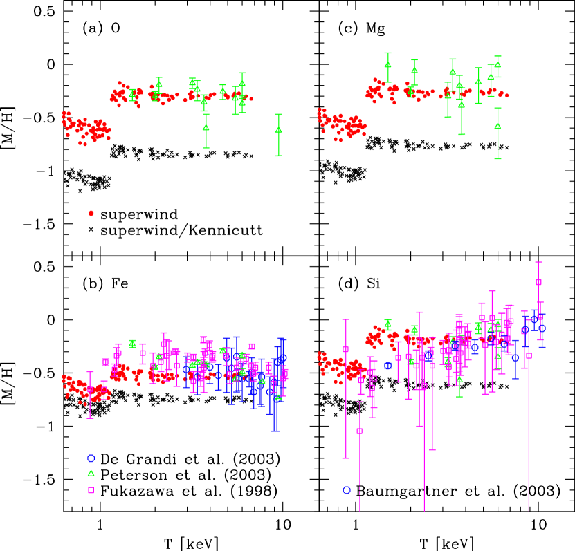
Figure 5: The metal abundances of the ICM, as predicted by a semi–analytical model of galaxy formation (from Nagashima et al. 2005). Each panel shows a different element: (a) [O/H], (b) [Fe/H], (c) [Mg/H] and (d) [Si/H]. Model predictions are shown by dots for a top-heavy IMF, and by crosses for the Kennicutt IMF. Symbols with error bars correspond to observational data, which have been taken from De Grandi et al. (2004), Peterson et al. (2003), Fukazawa et al. (1998) and Baumgartner et al. (2005) (see Nagashima et al. (2005) for details). All abundances have been rescaled to the Solar abundances by Grevesse & Sauval (1998).

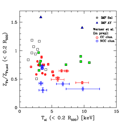
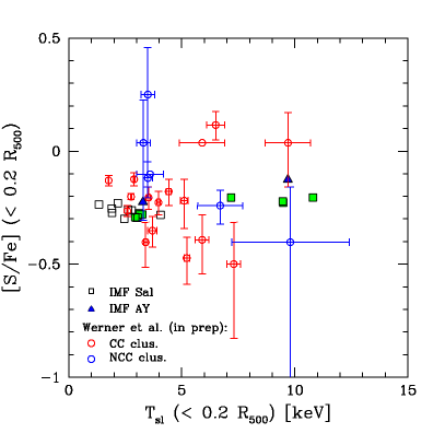
Figure 6: Left panel: the iron abundance within $0.2r_{500}$ as a function of the cluster temperature (here $r_{500}$ is defined as the radius encompassing an overdensity of $500\rho_{\rm c}$, with $\rho_{\rm c}$ the cosmic critical density). The open squares are for simulated clusters analysed by Fabjan et al. (in preparation), which assume a Salpeter IMF, while the filled triangles are for two simulated clusters which assume the top–heavy AY IMF. Open and filled circles with error bars are for cool–core and non cool–core clusters, respectively, observed with XMM–Newton by de Plaa et al. (2007) (see also Werner et al. 2008 - Chapter 16, this volume). Right panel: the same as in the left panel, but for the abundance of sulphur relative to iron. All abundances have been rescaled to the Solar abundances by Grevesse & Sauval (1998).

Based on a semi–analytical model of galaxy formation, Nagashima et al. (2005) carried out a comparison between the global observed and predicted ICM enrichment for different elements. In their analysis, these authors considered both the case of a “standard” Salpeter IMF and the case in which a top–heavier IMF is used in starbursts triggered by galaxy mergers. The comparison with observations, as reported in Fig. 5, led Nagashima et al. (2005) to conclude that the top–heavier IMF is required to reproduce the level of enrichment traced by different elements. All the abundances are predicted to be almost independent of temperature, at least for $T_{X}\gtrsim 1$ keV (this temperature corresponds to the limiting halo circular velocity, above which gas and metals ejected by superwinds are recaptured by the halo). While this result agrees with the observational points shown in the figure, they are at variance with respect to the significant temperature dependence of the iron abundance found by Baumgartner et al. (2005).

A different conclusion on the shape of the IMF is instead reached by other authors. For instance, Fabjan et al. (in preparation) analysed a set of hydrodynamical simulations of galaxy clusters, which include a chemical evolution model. In Fig. 6 we show the result of this analysis for the comparison between the simulated temperature dependence of iron (left panel) and sulphur (right panel) and the results of XMM–Newton observations by de Plaa et al. (2007) (see also Werner et al. 2008, - Chapter 16, this volume). As for the iron abundance, there is a tendency for simulations with a Salpeter IMF to overproduce this element, by about 30 per cent. Using a AY top–heavy IMF turns into a much worse disagreement, with an excess of iron in simulations by a factor 2–3. It is clear that this iron overabundance could be mitigated in case simulations include some mechanism for diffusion and/or mixing of metals, which decreases the abundance at small cluster-centric radii. Of course, this decrease should be such to reproduce the observed metallicity profiles (see below). As for the [S/Fe] relative abundance, the difference between the two IMFs is much smaller, since the two elements are produced in similar proportions by different stellar populations, and, within the relatively large observational uncertainties, they agree with data.

The comparison between the results of Figs. 5 and 6 is only one example of the different conclusions that different authors reach on the IMF shape from the study of the enrichment of the ICM. Tracing back the origin of these differences is not an easy task. Besides the different descriptions of the relevant physical processes treated in the SAMs and in the chemo–dynamical simulations, a proper comparison would also require using exactly the same model of chemical evolution and the same sets of yields for different stellar populations. We do recommend that all papers aimed at modelling the ICM enrichment should carefully include a complete description of the adopted chemical evolution model.

4 Metallicity profiles

Observations based on ASCA (e.g. Finoguenov et al. 2001) and Beppo–SAX (De Grandi et al. 2004) satellites have revealed for the first time the presence of significant gradients in the profiles of ICM metal abundances. The much improved sensitivity of the XMM–Newton and Chandra satellites are now providing much more detailed information on the spatial distributions of different metals, thus opening the possibility of shedding light on the past history of star formation in cluster galaxies and on the gas-dynamical processes which determine the metal distribution.

A detailed study of the metal distribution in the ICM clearly requires resorting to the detailed chemo-dynamical approach offered by hydrodynamical simulations. In principle, a number of processes, acting at different scales, are expected to play a role in determining the spatial distribution of metals: galactic winds (e.g. Tornatore et al. 2004; Romeo et al. 2006), transport by buoyant bubbles (Roediger et al. 2007; Sijacki et al. 2007), ram–pressure stripping (e.g., Kapferer et al. 2007b), diffusion by stochastic gas motions (Rebusco et al. 2005), sinking of highly enriched low–entropy gas (Cora 2006), etc. It is clear that modelling properly all such processes represents a non–trivial task for numerical simulations, which are required both to cover a wide dynamical range and to provide a reliable description of a number of complex astrophysical processes (Schindler & Diaferio 2008 - Chapter 17, this volume).

As an example, in the left panel of Fig. 7 we show the result of the analysis by Kapferer et al. (2007b), which was aimed at studying the relative role played by galactic winds and ram–pressure stripping in determining the metallicity profiles. In these simulations, based on an Eulerian grid code, these authors use a semi–analytical model to follow the formation and evolution of galaxies, and described the evolution of a global metallicity, instead of following different metal species. It is interesting to see how different mechanisms contribute in the simulations to establish the shape of the metallicity profile (see also Schindler & Diaferio 2008, - Chapter 17, this volume). In particular, ram–pressure stripping turns out to be more important in the central regions, where the pressure of the ICM is higher. On the other hand, galactic winds are more effective at larger radii, where they can travel for larger distances, thanks to the lower ICM pressure.

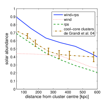
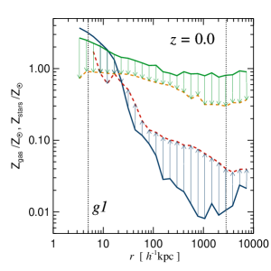
Figure 7: Left panel: contribution from ram–pressure stripping and from galactic winds to the resulting iron metallicity profile of a simulated cluster (from Kapferer et al. 2007b). Data points are from the Beppo–SAX observations analysed by De Grandi et al. (2004). Right panel: the effect of AGN feedback on the profiles of mass-weighted gas metallicity and stellar metallicity with simulations of a galaxy cluster (from Sijacki et al. 2007). Continuous lines show the metallicity profiles without AGN heating, while dashed lines are for the runs with AGN feedback. The arrows illustrate how the ICM metallicity is affected by the AGN feedback. The vertical dotted lines mark the resolution limit of the simulations and the virial radius of the simulated cluster.

As a further example, we show in the right panel of Fig. 7 the effect of AGN feedback on the distribution of metals in both gas and stars from the cluster simulations by Sijacki et al. (2007). These authors included in their SPH simulations a model for black hole growth and for the resulting energy feedback. Since these simulations do not include a detailed model of chemical evolution, the resulting metallicity cannot be directly compared to observations. Still, this figure nicely illustrates how the effect of AGN feedback is that of changing the share of metals between the stars and the gas. Due to the quenching of low–redshift star formation, a smaller amount of metals are locked back in stars, with a subsequent reduction of their metallicity. Furthermore, the more efficient metal transport associated to the AGN feedback causes a significant increase of the ICM metallicity in the outer cluster regions, thereby making the abundance profile shallower.

Since iron is the first element for which reliable profiles have been measured from X–ray observations, most of the comparisons performed so far with simulations have concentrated on its spatial distribution. As an example, we show in the left panel of Fig. 8 the comparison between the iron profiles measured by De Grandi et al. (2004) and results from the chemo–dynamical SPH simulations by Romeo et al. (2006). These authors performed simulations for two clusters having sizes comparable to those of the Virgo and of the Coma cluster, respectively. After exploring the effect of varying the feedback efficiency, they concluded that the resulting metallicity profiles are always steeper than the observed ones. A similar conclusion was also reached by Valdarnini (2003), based on SPH simulations of a larger ensemble of clusters, which used a rather inefficient form of thermal stellar feedback. A closer agreement between observed and simulated profiles of the iron abundance is found by Fabjan et al. (in preparation, see also Tornatore et al. 2007a), based on GADGET-2 SPH simulations, which include the effect of galactic winds, powered by SN explosions, according to the scheme presented by Springel & Hernquist (2003). The results of this comparison are shown in the right panel of Fig. 8. The solid black lines show the results for simulated clusters of mass in the range $\simeq(1-2)\times 10^{15}\,h^{-1}{\rm M}_{\odot}$, based on a Salpeter IMF, while the dashed curve is for one cluster simulated with a top–heavy AY IMF. The observational data points are for a set of nearby relaxed clusters observed with Chandra and for two clusters with $T\simeq 3$ keV observed with XMM–Newton. This comparison shows a reasonable agreement between simulated and observed profiles, with the XMM–Newton profiles staying on the low side of the Chandra profiles, also with a shallower slope in the central regions. While this conclusion holds when using a Salpeter IMF, a top–heavy IMF is confirmed to provide too high a level of enrichment.

The different degree of success of the simulations shown in the two panels of Fig. 8 in reproducing observations can have different origins. The most important reason is probably due to the different implementations of feedback which, as shown in Fig. 7, plays a decisive role in transporting metals away from star-forming regions. Another possible source of difference may lie in the prescription with which metals are distributed around star particles. Once again, the details of the numerical implementations of different effects need to be clearly specified in order to make it possible to perform a meaningful comparison among different simulations. Finally, it is also interesting to note that clusters observed with Chandra seem to have steeper central profiles than those observed with XMM–Newton and Beppo–SAX. There is no doubt that increasing the number of clusters with reliably determined metallicity profiles will help sorting out the origin of such differences.

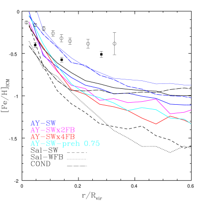
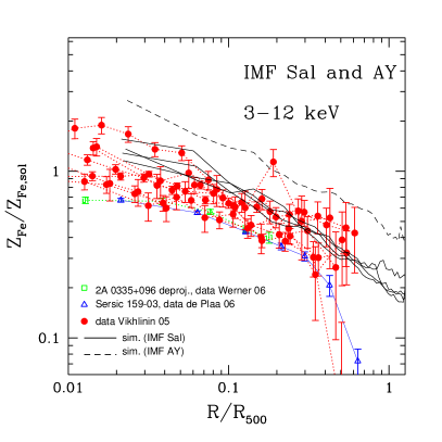
Figure 8: Left panel: profiles of iron metallicity at $z=0$ for different runs of two simulated clusters, obtained by changing the IMF (AY: Arimoto and Yoshii 1987; Sal: Salpeter 1955), the efficiency of the energy feedback and by including the effect of thermal conduction (COND; from Romeo et al. 2005). Observational data points are taken from De Grandi et al. (2004). Right panel: Comparison between observed and simulated profiles of iron abundance (from Fabjan et al., in preparation). The continuous black curves are for four simulated clusters, having virial masses in the range $(1-2)\times 10^{15}\,h^{-1}{\rm M}_{\odot}$, assuming a Salpeter IMF. The black dashed line is for one of these clusters, simulated by assuming the AY top–heavy IMF. Filled circles with error bars shows observational results from Chandra (Vikhlinin et al. 2005) for clusters with temperature above 3 keV, while the open squares and triangles are for the profiles of two $\simeq 3$ keV clusters observed with XMM–Newton (de Plaa et al. 2006; Werner et al. 2006). The iron abundance has been rescaled to the Solar abundances by Grevesse & Sauval (1998).

5 Evolution of the ICM metallicity

After the pioneering paper based on ASCA data by Mushotzky & Loewenstein (1997), the increased sensitivity of the XMM–Newton and Chandra observatories recently opened the possibility of tracing the evolution of the global iron content of the ICM out to the largest redshifts, $z\simeq 1.4$, where clusters have been secured (e.g. Balestra et al. 2007; Maughan et al. 2007). These observations have shown that the ICM iron metallicity decreases by about 50 per cent from the nearby Universe to $z\simeq 1$. This increase of metallicity at relatively recent cosmic epochs can be interpreted as being due either to a fresh production of metals or to a suitable redistribution of earlier-produced metals. Since SN Ia, which provide a large contribution to the total iron budget, can release metals over fairly long time scales, the increase of the iron abundance at $z<1$ is not necessarily in contradiction with the lack of recent star formation in the bulk of cluster galaxies. On the one hand, recent analyses (Ettori 2005; Loewenstein 2006) have shown that the observed metallicity evolution is consistent with the observed SN Ia rate in clusters (Gal-Yam et al. 2002). On the other hand, a number of processes, such as stripping of metal enriched gas from merging galaxies (e.g., Calura et al. 2007) or sinking of highly enriched low–entropy gas towards the cluster central regions (Cora 2006) may also significantly contribute to the ICM metallicity evolution, through a redistribution of enriched gas. Indeed, the amount of accreted gas since $z=1$ is at least comparable to that present within the cluster at that redshift. Therefore, the evolution of the ICM metallicity is expected to be quite sensitive to the enrichment level of the recently accreted gas. On the other hand, as noted by Renzini (1997), if ram–pressure stripping plays a dominant role in determining the ICM enrichment, one should then expect to observe more massive clusters, whose ICM has a higher pressure, to be more metal rich than poorer systems. In fact, observations do not show this trend and, if any, suggest a decrease of the iron abundance with the ICM temperature (e.g., Baumgartner et al. 2005).

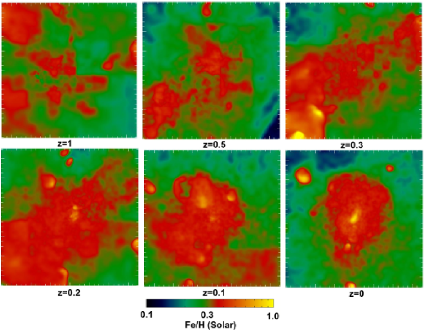
Figure 9: Evolution of the iron abundance within 700 $h^{-1}$ kpc from the centre of a simulated cluster at $z=1,0.5,0.3,0.2,0.1,0$, from upper left to bottom right panel. The maps show the projection of the mass–weighted iron abundance by number relative to hydrogen, Fe/H, with respect to the solar value (adapted from Cora 2006).

Cora (2006) used a hybrid approach based on coupling a SAM model of galaxy formation to a non–radiative hydrodynamical simulation to study the gas dynamical effects which lead to the re-distribution of metals from the star forming regions. The results of her analysis are summarised in the metallicity maps shown in Fig. 9. Metals are produced inside small halos which at high redshift define the proto–cluster region. Since the gas in these halos has undergone no significant shocks by diffuse accretion, its entropy is generally quite low. This low–entropy highly enriched gas is therefore capable to sink towards the central regions of the forming cluster. As a consequence, this leads to an increase of the metallicity in the regions which mostly contribute to the emissivity, thereby causing a positive evolution of the observed metallicity.

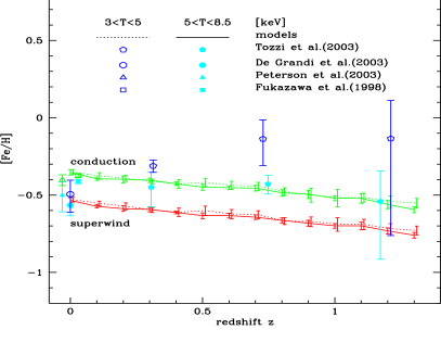
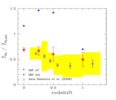
Figure 10: The redshift evolution of the iron abundance. Left panel: predictions by different flavours of the SAM by Nagashima et al. (2005), based on a top–heavy IMF, compared with observational data from different sources, for clusters within two temperature ranges. Error bars on model predictions are the 1$\sigma$ scatter over the ensemble of cluster formation histories. Right panel: comparison between observational data and full hydrodynamical simulations by Fabjan et al. (2007, in preparation). Open circles come from the analysis of Chandra data by Balestra et al. (2007). The shaded area represents the r.m.s. scatter within each redshift interval, while the error bars are the 1$\sigma$ confidence level. The filled squares are for a set of four simulated clusters, using a Salpeter IMF, with temperature ${\mathrm{k}}T>5$ keV, with error bars indicating the corresponding 1$\sigma$ scatter. The filled triangles refer to only one cluster, out of four, simulated with the top–heavy IMF. In both panels, the values of the iron abundance have been rescaled to the Solar abundances by Grevesse & Sauval (1998).

Nagashima et al. (2005) used a SAM approach, not coupled to hydrodynamical simulations, to predict the evolution of the ICM metallicity. In this case, the evolution is essentially driven by the low–redshift star formation, since any redistribution of enriched gas is not followed by the model. The result of their analysis (left panel of Fig. 10) shows that a very mild evolution is predicted. A prediction of the evolution of the iron abundance from hydrodynamical simulations, which self–consistently follow gas cooling, star formation and chemical evolution, has been more recently performed by Fabjan et al. (in preparation). The results of their analysis are shown in the right panel of Fig. 10, where they are also compared to the observational results by Balestra et al. (2007). Also in this case, the results based on a Salpeter IMF are in reasonable agreement with observations, while a top–heavier IMF produces too high metallicities at all redshifts. Quite interestingly, at low redshift the run with top–heavy IMF shows an inversion of the evolution. This is due to the exceedingly high star formation triggered by heavily enriched gas, which locks back in stars a substantial fraction of the gas metal content in the cluster central regions. This highlights the crucial role played by star formation in both enriching the ICM and in locking back metals in the stellar phase. This further illustrates how the resulting metallicity evolution must be seen as the result of a delicate interplay of a number of processes, which all need to be properly described in a self–consistent chemo–dynamical model of the ICM.

6 Properties of the galaxy population

The physical processes which determine the thermodynamical and chemical properties of the ICM are inextricably linked to those determining the pattern of star formation in cluster galaxies. For this reason, a successful description of galaxy clusters requires a multiwavelength approach, which is able at the same time to account for both the X–ray properties of the diffuse hot gas and of the optical/near–IR properties of the galaxy populations. In this sense, the reliability of a numerical model of the ICM chemical enrichment is strictly linked to its ability to reproduce the basic properties of the galaxy population, such as luminosity function and colour–magnitude diagram. While the study of the global properties of the galaxy populations has been conducted for several years with semi–analytical models of galaxy formation (De Lucia et al. 2004; Nagashima et al. 2005), it is only quite recently that similar studies have been performed with cosmological hydrodynamical simulations, thanks to the recent advances in supercomputing capabilities and code efficiency.

As we have already mentioned, hydrodynamical simulations treat the process of star formation through the conversion of cold and dense gas particles into collisionless star particles. Each star particle is then characterised by a formation epoch and a metallicity. Therefore, it can be treated as a SSP, for which luminosities in different bands can be computed by resorting to suitable stellar population synthesis models. Since the colours of a SSP are quite sensitive to metallicity, it is necessary for simulations to include a detailed chemical evolution model in order to reliably compare predictions on optical/near–IR properties of galaxies with observational data. This approach has been pursued by Kawata & Gibson (2003b), who performed simulations of elliptical galaxies and by Romeo et al. (2005) and Saro et al. (2006), who performed simulations of galaxy clusters. The results of these analyses are summarised in Fig. 11. In the left panels we show the position on the colour–magnitude diagram of the elliptical galaxies simulated by Kawata & Gibson (2003b). This plot clearly indicates that elliptical galaxies are generally much bluer than observed, as a result of an excess of recent star formation, which is not properly balanced by an efficient feedback mechanism. Indeed, it is only after excluding the contribution from recently formed stars that Kawata & Gibson (2003b) were able to obtain ellipticals with more realistic colours.

Figure 11: Left panel: Colour–magnitude relations for the simulations of elliptical galaxies (Kawata & Gibson 2003b), based on a Salpeter IMF, compared to the observational results for the galaxies in Coma (Bower et al. 1992) (crosses) and for NGC 4472 (open star). The filled square and circle are the results for the reference runs, whereas the open symbols are when the contribution from stars younger than 2 or 8 Gyr are ignored. Right panel: the colour–magnitude relation for simulated clusters (symbols). Upper and lower panels refer to simulations performed with a Salpeter IMF and with the AY IMF, respectively (from Saro et al. 2006). The big dots are for the BCGs of the simulated clusters. The straight lines indicate the best-fitting relation and the scatter observed for the Coma galaxies.

In the right panels we show the colour–magnitude relation (CMR) of the galaxy population of an extended set of clusters simulated by Saro et al. (2006) based both on a Salpeter IMF and on a top–heavy IMF. Quite apparently, the bulk of the galaxy population traces a CMR which is consistent with the observed one, at least for a Salpeter IMF. As for the top–heavy IMF, it predicts too red colours as a consequence of a too high metal content of galaxies. Also interesting to note, brighter redder galaxies are on average more metal rich, therefore demonstrating that the CMR corresponds in fact to a metallicity sequence (see also Romeo et al. 2005). However, a clear failure of these simulations is that the BCGs are always much bluer than observed. This result agrees with the exceedingly blue colour of simulated ellipticals shown in the left panels. This is due to an excess of recent star formation, which, in BCGs of $\sim 10^{15}M_{\odot}$ simulated clusters, can be as high as 500–1000 M_⊙ yr^-1. As discussed by Borgani et al. 2008 - Chapter 13, this volume, the presence of overcooling in cluster simulations manifests itself with the presence of steep negative temperature gradients in the central regions. In this sense, wrong BCG colours and temperature profiles in core regions are two aspects of the same problem, i.e. the difficulty of balancing the cooling runaway within simulated clusters.

Since all these simulations include recipes for stellar feedback, although with different implementations and efficiencies, the solution to the overcooling in clusters should be found in some non–stellar feedback, such as that provided by AGN. Recent studies of the galaxy properties, based on semi–analytical models, have shown that an energy feedback of the sort of that expected from AGN, is able to suppress the bright end of the galaxy luminosity function, which is populated by the big ellipticals residing at the centre of clusters (e.g., Bower et al. 2006; Croton et al. 2006). There is no doubt that providing robust predictions on the properties of the galaxy population will be one of the most important challenges for simulations of the next generation to be able of convincingly describing the thermo- and chemo-dynamical properties of the hot gas.

7 Summary

The study of the enrichment pattern of the ICM and its evolution provides a unique means to trace the past history of star formation and the gas–dynamical processes, which determine the evolution of the cosmic baryons. In this overview, we discussed the concept of model of chemical evolution, which represents the pillar of any chemo–dynamical model, and presented the results obtained so far in the literature, based on different approaches. Restricting the discussion to those methods which follow the chemical enrichment during the cosmological assembly of galaxies and clusters of galaxies, they can be summarised in the following categories.
(1) Semi–analytical models (SAMs) of galaxy formation (De Lucia et al. 2004; Nagashima et al. 2005): the production of metals is traced by the history of galaxy formation within the evolving DM halos and no explicit gas–dynamical description of the ICM is included. These approaches are computationally very cheap and provide a flexible tool to explore the space of parameters determining galaxy formation and chemical evolution. A limitation of these approaches is that, while they provide predictions on the global metal content of the ICM, the absence of any explicit gas dynamical description causes the lack of useful information on the spatial distribution of metals.
(2) SAMs coupled to hydrodynamical simulations. In this case, the galaxy formation is followed as in the previous approach, but the coupling with a hydrodynamical simulation allows one to trace the fate of the enriched gas and, therefore, to study the spatial distribution of metals. Different authors have applied different implementations of this hybrid approach, by focusing either on the role of the chemical evolution model (Cora 2006) or on the effect of specific gas–dynamical processes, such as ram–pressure stripping and galactic winds, in enriching the ICM (e.g., Kapferer et al. 2007b). The advantage of this approach is clearly that gas–dynamical processes are now included at some level. However, the galaxy formation process is not followed in a self–consistent way from the cooling of the gas during the cosmic evolution.
(3) Full hydrodynamical simulations, which self–consistently follow gas cooling, star formation and chemical evolution (Valdarnini 2003; Kawata & Gibson 2003b; Romeo et al. 2005; Tornatore et al. 2007a). Rather than being described by an external recipe, galaxy formation is now the result of the cooling and of the conversion of cold dense gas into stars, as implemented in the simulation code. The major advantage of this approach is that the enrichment process now comes as the result of the star formation predicted by the hydrodynamical simulation, without resorting to any external model. The bottleneck, in this case, is represented by the computational cost, which becomes prohibitively high if one wants to resolve the whole dynamic range covered by the processes of metal production and distribution, feedback energy release, etc. For this reason, these simulation codes also need to resort to sub–resolution models, which provide an effective description of a number of physical processes. However, there is no doubt that the ever improving supercomputing technology and code efficiency make, in perspective, this approach the way to study the past history of cosmic baryons.

As already emphasised, developing a reliable model of the cosmic history of metal production is a non–trivial task. This is due to the sensitive dependence of the model predictions on both the parameters defining the chemical evolution model (i.e., IMF, stellar life–times, stellar yields, etc.), and on the processes, such as ejecta from SN explosions and AGN, stripping, etc., which at the same time regulate star formation and transport metals outside galaxies. In the light of these difficulties, it is quite reassuring that the results of the most recent hydrodynamical simulations are in reasonable agreement with the most recent observational data from Chandra and XMM–Newton.

In spite of this success, cluster simulations of the present generation still suffer from important shortcomings. The most important of them is probably represented by the difficulty in regulating overcooling at the cluster centre, so as to reproduce at the same time the observed “cool cores” and the passively evolving massive ellipticals. Besides improving the description of the relevant astrophysical processes in simulation codes, another important issue concerns understanding the possible observational biases which complicate any direct comparison between data and model predictions (Kapferer et al. 2007a; Rasia et al. 2007). In this respect, simulations provide a potentially ideal tool to understand these biases. Mock X–ray observations of simulated clusters, which include the effect of instrumental response, can be analysed exactly in the same way as real observational data. The resulting “observed” metallicity can then be compared with the true one to calibrate out possible systematics. There is no doubt that observations and simulations of the chemical enrichment of the ICM should go hand in hand in order to fully exploit the wealth of information provided by X–ray telescopes of the present and of the next generation.