$q$-breathers in Discrete Nonlinear Schrödinger lattices

Abstract

$q$-breathers are exact time-periodic solutions of extended nonlinear systems continued from the normal modes of the corresponding linearized system. They are localized in the space of normal modes. The existence of these solutions in a weakly anharmonic atomic chain explained essential features of the Fermi-Pasta-Ulam (FPU) paradox. We study $q$-breathers in one- two- and three-dimensional discrete nonlinear Schödinger (DNLS) lattices — theoretical playgrounds for light propagation in nonlinear optical waveguide networks, and the dynamics of cold atoms in optical lattices. We prove the existence of these solutions for weak nonlinearity. We find that the localization of $q$-breathers is controlled by a single parameter which depends on the norm density, nonlinearity strength and seed wave vector. At a critical value of that parameter $q$-breathers delocalize via resonances, signaling a breakdown of the normal mode picture and a transition into strong mode-mode interaction regime. In particular this breakdown takes place at one of the edges of the normal mode spectrum, and in a singular way also in the center of that spectrum. A stability analysis of $q$-breathers supplements these findings. For three-dimensional lattices, we find $q$-breather vortices, which violate time reversal symmetry and generate a vortex ring flow of energy in normal mode space.

I Introduction

I.1 Background

In 1955, Fermi, Pasta and Ulam (FPU) published their seminal report on the absence of thermalization in arrays of particles connected by weakly nonlinear springs fpu . In particular they observed that energy, initially seeded in a low-frequency normal mode of the linear problem with a frequency $\omega_{q}$ and corresponding normal mode number $q$, stayed almost completely locked in a few neighbor modes in frequency space, instead of being distributed quickly among all modes of the system. The latter expectation was due to the fact, that nonlinearity does induce a long-range network of interactions among the normal modes. ¿From the present perspective, the FPU problem appears to consist of the following parts: (i) for certain parameter ranges (energy, system size, nonlinearity strength, seed mode number), excitations appear to stay exponentially localized in $q$-space of the normal modes for long but finite times lgas72 ; (ii) this intermediate localized state is reached on a fast time scale $\tau_{1}$, and equipartition is reached on a second time scale $\tau_{2}$, which can be many orders of magnitude larger than $\tau_{1}$ GIORGILLI SHOWERS ; (iii) tuning the control parameters may lead to a drastical shortening of $\tau_{2}$, until both time scales merge, and the metastable regime of localization is replaced by a fast relaxation towards thermal equilibrium GIORGILLI SHOWERS , which is related to the nonlinear resonance overlap estimate by Izrailev and Chirikov fmibvc66 . FPU happened to compute cases with values of $\tau_{2}$ which were inaccessible within their computation time. Among many other intriguing details of the evolution of the intermediate localized state, we mention the possibility of having an almost regular dynamics of the few strongly excited modes, leading to the familiar phenomenon of beating. That beating manifests as a recurrence of almost all energy into the originally excited mode (similar to the beating among two weakly coupled harmonic oscillators), and was explained by Zabusky and Kruskal with the help of real space solitons of the Kordeweg-de-Vries (KdV) equation, for a particular case of long wavelength seed modes, and periodic boundary conditions njzmdk65 . The regular dynamics may be replaced by a weak chaotic one upon crossing yet another threshold in control parameters jdlalmal95 . Remarkably, that weak chaos is still confined to the core of the localized excitation, leaving the exponential localization almosts unchanged, and perhaps influencing most strongly the parameter dependence of $\tau_{2}$. The interested reader may also consult Ref.fpumore .

I.2 Motivation

Single-site excitations in translationally invariant lattices of interacting anharmonic oscillators are known to show a similar behaviour of trapping the excitation on a few lattice sites around the originally excited one dbnumerics . As conjectured almost 40 years ago ovchinnikov , exact time-periodic and spatially localized orbits - discrete breathers (also intrinsic localized modes, discrete solitons) persist in such lattices, and the dynamics on such an orbit, as well as the dynamics of the nearby phase space flow, account for many observations, and have found their applications in many different areas of physics db . Recently, it was shown, that the regime of localization in normal mode space for the FPU problem can be equally explained by obtaining $q$-breathers (QB) - time-periodic and modal-space-localized orbits - which persist in the FPU model for nonzero nonlinearity QB . The originally computed FPU trajectory stays close to such $q$-breather solutions for long times, and therefore many features of its short- and medium-time dynamics have been shown to be captured by the $q$-breather solution and small phase-space fluctuations around it. Delocalization thresholds for $q$-breathers are related to resonances, and corresponding overlap criteria QB . The method of constructing $q$-breather solutions was generalized to two- and three-dimensional FPU lattices FPU2d3d . Most importantly, a scaling theory was developed, which allowed to construct $q$-breathers for arbitrarily large system sizes, and to obtain analytical estimates on the degree of localization of these solutions for macroscopic system size Scaling . Expectations were formulated, that the existence of $q$-breathers should be generic to many nonlinear spatially extended systems.

I.3 Aim

The spectrum of normal mode frequencies of the linear part of the FPU model is acoustic, contains zero, reflecting the fact, that the model conserves total mechanical momentum. In addition it is bounded by a lattice-induced cutoff, the analogue of the Debye cutoff in solid state physics. We may think of two pathways of extending the above discussed results to other system classes. First, we could consider a spatially continuous system, instead of a lattice. However, the initial FPU studies showed confinement to a few long wavelength modes, and the results of Zabusky and Kruskal njzmdk65 , confirm, that indeed in the spatially continuous system (KdV), trajectories similar to the FPU trajectory persist.

As discussed above, the persistence, localization, and delocalization of $q$-breathers is due to a proper avoiding of, or harvesting on, resonances between normal modes. It therefore appears to be of substantial interest to extend the previous results to systems with a qualitatively different normal mode spectrum. Such a spectrum is one which does not contain zero, and is called optical. It may correspond to the excitation of certain degrees of freedom in a complex system, or to an FPU type model which is deposited on some substrate, or otherwise exposed to some external fields. Together with the acoustic band, these two band structures, when combined, describe almost any type of normal mode spectrum in a linear system with spatially periodic modulated characteristics.

Adding weak nonlinearities to such a system, taking local action angle representations, and performing various types of multiple scale analysis, such models are mapped on discrete nonlinear Schrödinger models (DNLS) DNLS derivations . These models enjoy a gauge invariance, and a conservation of the sum of the local actions (norms), i.e. some global norm. A particular version of these equations is known as the discrete Gross-Pitaevsky equation, and is derived on mean field grounds for Bose-Einstein condensates of ultracold bosonic atoms in optical lattices grosspitaevsky ; healinglength . The norm is simply the conserved number of atoms in this case, and the nonlinearity derives from the atom-atom interaction. The propagation of light in (spatially modulated) optical media is another research area where DNLS models are used nonlinearoptics . In that case the norm conservation derives from the conservation of electromagnetic wave energy along the propagation distance (in the assumed absence of dissipative mechanisms). But DNLS models served equally well in many other areas of physics, where weak interactions start to play a role, e.g. in the theory of polaron formation due to electron-phonon interaction in solids.

Releasing the norm conservation (e.g. by allowing the number of atoms in a condensate to fluctuate) will reduce the symmetries of the corresponding model, but most importantly, it will lead to possible new resonances of higher harmonics. We will discuss these limitations, and possible effects of releasing these limitations on $q$-breathers, in the discussion section.

A particular consequence of norm conservation is a corresponding symmetry of the normal mode spectrum, which relates both (upper and lower) band edges, and makes the band center a symmetry point as well.

The paper is structured as follows. Section II is introducing the model and the main equations of motion. Section III gives an existence proof for $q$-breathers. In section IV we derive analytical expressions for the QB profiles using perturbation theory. These are compared with the numerical results for $d=1$ in section V, which also contains a stability analysis of the obtained periodic orbits. Section VI gives results on periodic boundary conditions (as opposed to fixed boundaries). We generalize to $d=2,3$ in section VII, and discuss all results in section VIII.

II Model

We consider a discrete nonlinear Schrödinger (DNLS) equation on a $d$-dimensional hypercubic lattice of linear size $N$:

$$i\dot{\psi_{\boldsymbol{n}}}=\sum\limits_{\boldsymbol{m}\in D(\boldsymbol{n})}\psi_{\boldsymbol{m}}+\mu|\psi_{\boldsymbol{n}}|^{2}\psi_{\boldsymbol{n}}.$$ (1)

Here $\psi$ is a complex scalar which may describe e.g. the probability amplitude of an atomic cloud on an optical lattice site healinglength , or relates to the amplitudes of a propagating electromagnetic wave in an optical waveguide nonlinearoptics . The lattice vectors $\boldsymbol{n,m}$ have integer components, and $D(\boldsymbol{n})$ is the set of nearest neighbors for the lattice site $\boldsymbol{n}$. If not noted otherwise, we consider fixed boundary conditions: $\psi_{\boldsymbol{n}}=0$ if $n_{l}=0$ or $n_{l}=N+1$ for any of the components of $\boldsymbol{n}$. Equation (1) is derived from the Hamiltonian

$$H=\sum\limits_{\boldsymbol{n}}\left(\sum\limits_{\boldsymbol{m}\in D(\boldsymbol{n})}\psi_{\boldsymbol{m}}\psi_{\boldsymbol{n}}^{*}+\frac{\mu}{2}|\psi_{n}|^{4}\right)$$ (2)

using the equations of motion $i\dot{\psi_{n}}=\partial H/\partial\psi_{n}^{*}$. In addition to energy, equation (1) conserves the norm $B=\sum\limits_{\boldsymbol{n}}|\psi_{\boldsymbol{n}}|^{2}$. Note that the change of the nonlinearity parameter $\mu$ in (1) is strictly equivalent to changing the norm $B$. Here we will keep the norm $B$ (alternatively the norm density) fixed, and vary $\mu$.

We perform a canonical transformation to the reciprocal space of normal modes ($q$-space of size $N^{d}$) with new variables $Q_{\boldsymbol{q}}(t)\equiv Q_{q_{1}\ldots q_{d}}(t)$

$$\psi_{\boldsymbol{n}}(t)=\left(\frac{2}{N+1}\right)^{d/2}\sum\limits_{q_{1},\ldots,q_{d}=1}^{N}Q_{\boldsymbol{q}}(t)\prod\limits_{i=1}^{d}\sin{\left(\frac{\pi q_{i}n_{i}}{N+1}\right)}\;.$$ (3)

Together with (1) we obtain the following equations of motion in normal mode space:

$$i\dot{Q_{\boldsymbol{q}}}=-\omega_{\boldsymbol{q}}Q_{\boldsymbol{q}}+\frac{2^{d-2}\mu}{(N+1)^{d}}\sum\limits_{\boldsymbol{p,r,s}}C_{\boldsymbol{q,p,r,s}}Q_{\boldsymbol{p}}Q_{\boldsymbol{r}}^{*}Q_{\boldsymbol{s}},$$ (4)

where $\omega_{\boldsymbol{q}}=-2\sum\limits_{i=1}^{d}\cos{\frac{\pi q_{i}}{N+1}}$ are the normal mode frequencies for the linearized system (1) with $\mu=0$. Nonlinearity introduces a network of interactions among the normal mode oscillators with the following coupling coefficients:

$$\begin{array}[]{c}C_{\boldsymbol{q,p,r,s}}=\prod\limits_{i=1}^{d}C_{q_{i},p_{i},r_{i},s_{i}},\\ C_{q_{i},p_{i},r_{i},s_{i}}=\sum\limits_{k,l,m=0}^{1}(-1)^{k+l+m}(\delta_{(-1)^{k}p_{i}+(-1)^{l}r_{i}+(-1)^{m}s_{i},q_{i}}+\\ +\delta_{(-1)^{k}p_{i}+(-1)^{l}r_{i}+(-1)^{m}s_{i},q_{i}\pm(2N+2)}).\end{array}$$ (5)

III Proof of existence of $t$-reversible $q$-breather solutions for weak nonlinearity

We look for exact time-periodic solutions, which are stationary solutions of the DNLS equation (1), and which are localized in normal mode space: $\psi_{\boldsymbol{n}}(t)=\phi_{\boldsymbol{n}}exp(i\Omega t)$ with frequency $\Omega$ and time-independent amplitudes $\phi_{\boldsymbol{n}}$. In the space of normal modes these stationary solutions have the form $Q_{\boldsymbol{q}}(t)=A_{\boldsymbol{q}}exp(i\Omega t)$, where the amplitudes of modes $A_{\boldsymbol{q}}$ are time-independent and related to the real-space amplitudes by the transformation (3). At a given norm $B$ they satisfy a system of algebraic equations:

$$\left\{\begin{array}[]{lc}-\Omega A_{\boldsymbol{q}}+\omega_{\boldsymbol{q}}A_{\boldsymbol{q}}-\frac{2^{d-2}\mu}{(N+1)^{d}}\sum\limits_{\boldsymbol{p},\boldsymbol{r},\boldsymbol{s}}C_{\boldsymbol{q},\boldsymbol{p},\boldsymbol{r},\boldsymbol{s}}A_{\boldsymbol{p}}A^{*}_{\boldsymbol{r}}A_{\boldsymbol{s}}=0,&q_{1,..,d}=\overline{1,N},\\ \sum\limits_{\boldsymbol{q}}|A_{\boldsymbol{q}}|^{2}-B=0,&\end{array}\right.$$ (6)

We are focusing here (and throughout almost all of the paper) on $t$-reversible periodic orbits. Therefore we may consider all $A_{\boldsymbol{q}}$ to be real numbers. In this case system (6) contains $N+1$ equations for $N+1$ variables. This system can be condensed into an equation for a vector function:

$$\boldsymbol{F}(\boldsymbol{X};\mu,B)=0$$ (7)

with $\boldsymbol{X}=\{\ldots,A_{\boldsymbol{q}},\ldots,\Omega\}$. The components of $\boldsymbol{F}$ are the left hand sides of (6), while $\mu$, $B$ are parameters.

For $\mu=0$ the normal modes in (4) are decoupled and each oscillator conserves its norm in time: $B_{\boldsymbol{q}}(t)=A_{\boldsymbol{q}}^{2}$. Let us consider the excitation of only one of the oscillators with the seed mode number $\boldsymbol{q}_{0}$: $B_{\boldsymbol{q}}=B_{\boldsymbol{q}_{0}}\delta_{\boldsymbol{q},\boldsymbol{q}_{0}}$. The excited normal mode is a time-periodic solution of (4), and is localized in $\boldsymbol{q}$-space. According to the Implicit Function Theorem ImpFunc , the corresponding solution of (6) can be continued into the nonlinear case ($\mu\neq 0$), if the Jacoby matrix of the linear solution $(\partial\boldsymbol{F}/\partial\boldsymbol{X})_{\mu=0,B}$ is invertible, i.e. $||\partial\boldsymbol{F}/\partial\boldsymbol{X}||_{\mu=0,B}\neq 0$. The Jacobian

$$\left\|{\frac{\partial\mathbf{F}}{\partial\mathbf{X}}}\right\|_{\mu=0}=(-1)^{N^{d}+1}2A_{\boldsymbol{q}_{0}}^{2}\prod\limits_{\boldsymbol{q}\neq\boldsymbol{q}_{0}}(\omega_{\boldsymbol{q}}-\omega_{\boldsymbol{q}_{0}}).$$ (8)

Invertibility of the Jacoby matrix requires a non-degenerated spectrum of normal mode frequencies. Therefore, the continuation of a linear mode with the seed mode number $\boldsymbol{q}_{0}$ will be possible if $\omega_{\boldsymbol{q}}\neq\omega_{\boldsymbol{q}_{0}}$, for all $\boldsymbol{q}\neq\boldsymbol{q}_{0}$. That condition holds for the case $d=1$, and thus $q$-breathers exist at least for suitably small values of $\mu$ there. For higher dimensions, degeneracies of normal mode frequencies appear. These degeneracies are not an obstacle for numerical continuation of $q$-breathers, but a formal persistence proof has to deal with them accordingly. Analogous results for two- and three-dimensional $\beta$-FPU lattices have been obtained in Ref. FPU2d3d .

IV Perturbation theory for $q$-breather profiles

To analyze the localization properties of $q$-breathers in $q$-space we use a perturbation theory approach similar to QB ,FPU2d3d . We consider the general case of a $d$-dimensional DNLS lattice (1). Taking the solution for a linear normal mode with number $\boldsymbol{q}_{0}=(q_{1,0},\ldots,q_{d,0})$ as a zero-order approximation, an asymptotic expansion of the solution to the first $N$ equations of (6) in powers of the small parameter $\sigma=\mu 2^{(d-2)}/(N+1)^{d}$ is implemented. Note, that in the same way as it was done in QB ,FPU2d3d , we fix the amplitude of the seed mode $A_{\boldsymbol{q}_{0}}$. Later on we will apply the norm conservation law (the last equation of (6)) to express the norm $B_{\boldsymbol{q}_{0}}=|A_{\boldsymbol{q}_{0}}|^{2}$ via the total norm $B$ for the case of $d=1$. Analytical estimations presented below describe amplitudes of modes located along the directions of the lattice axes starting from the mode $\boldsymbol{q}_{0}$. Mode amplitudes of $q$-breathers have the slowest decay along these directions. Studying $q$-breather localization along a chosen dimension $i$, for the sake of compactness we will use a scalar mode number to denote the $i$-th component of $\boldsymbol{q}$, assuming all other components be the same as in $\boldsymbol{q}_{0}$: $q_{j\neq i}=q_{j,0}$.

IV.1 Close to the band edges

Let us start with $q$-breathers localized in the low-frequency mode domain ($q_{i,0}<<N$, $i=\overline{1,d}$). According to the selection rules, if the seed mode number $q_{i,0}$ is even (odd), then only even (odd) modes are excited along $i$-th dimension. The $n$-th order of the asymptotic expansion is the leading one for the mode $q_{i,n}=(2n+1)q_{i,0}$. When $q_{i}$ reaches the upper band edge in the $i$-th direction, a reflection at the edge in $q$-space takes place if $N+1$ is not divisible by $q_{i,0}$ (cf. Fig. 1d). If $N+1$ is divisible by $q_{i,0}$ then only modes $q_{i,n}=(2n+1)q_{i,0}<N$ are excited. In the analytical estimates we assume a large enough lattice size. Then the effect of band edge reflections is appearing in higher orders of the perturbation, which will not be considered. In this case the approximate solution is

$$A_{(2n+1)q_{i,0}}=(-\mbox{sign}(\mu))^{n}\left(\sqrt{\lambda_{d}^{(i)}}\right)^{n}A_{\boldsymbol{q}_{0}}\;,\;i=\overline{1,d}\;,\;\Omega=\omega_{\boldsymbol{q}_{0}}-\sigma A_{\boldsymbol{q}_{0}}^{2}+O(\sigma^{2})\;.$$ (9)

The corresponding exponential decay of mode norms is

$$B_{(2n+1)q_{i,0}}=(\lambda_{d}^{(i)})^{n}B_{\boldsymbol{q}_{0}}\;,\;\sqrt{(\lambda_{d}^{(i)})}=\frac{|\mu|A_{\boldsymbol{q}_{0}}^{2}(N+1)^{2-d}}{2^{5-d}\pi^{2}{(q_{i,0})}^{2}}=\frac{|\mu|b_{\boldsymbol{k}_{0}}}{2^{5-d}{(k_{i,0})}^{2}}\;,\;i=\overline{1,d}\;.$$ (10)

$\lambda_{d}^{(i)}$ ($0<\lambda_{d}^{(i)}<1$) characterize the exponential decay along the $i$-th dimension. Here $k_{i,0}=\frac{\pi q_{i,0}(2n+1)}{N+1}<\pi$ is the $i$-th component of the seed wave vector $\boldsymbol{k}_{0}$, and $b_{\boldsymbol{k}_{0}}=B_{\boldsymbol{k}_{0}}/(N+1)^{d}$ is the norm density of the seed mode. When using intensive quantities – wave number $k_{i,0}$ and norm density $b_{\boldsymbol{k}_{0}}$ – only, $\lambda$ does not depend on the system size.

Equations (4) are invariant under the symmetry operation $\mu\rightarrow-\mu$, $t\rightarrow-t$, $q_{i,0}\rightarrow N+1-q_{i,0}$ for all $i=\overline{1,d}$, which changes the sign of nonlinearity, and maps modes from one band edge to the other. The replacement $q_{i,0}\rightarrow N+1-q_{i,0}$ for all $i=\overline{1,d}$ in (6) is equivalent to substitutions $\mu\rightarrow-\mu$ and $\Omega\rightarrow-\Omega$. Using this symmetry, we can easily apply the above results to the case of $q$-breathers localized near the upper band edge, by counting mode indices from the upper edge: $\widetilde{q}_{i}=N+1-q_{i}$. We neglect reflections from the lower band edge, such that only modes with numbers $\widetilde{q}_{i,n}=(2n+1)\widetilde{q}_{i,0}$ ($n$ is integer, $\widetilde{q}_{i,0}<<N$) are assumed to be excited. It follows

$$A_{N+1-\widetilde{q}_{i,n}}=(\mbox{sign}(\mu))^{n}\left(\sqrt{\widetilde{\lambda}_{d}^{(i)}}\right)^{n}A_{\boldsymbol{q}_{0}}$$ (11)

where $n$ is an integer and

$$\begin{array}[]{cc}\sqrt{(\widetilde{\lambda}_{d}^{(i)})}=\frac{|\mu|A_{\boldsymbol{q}_{0}}^{2}(N+1)^{2-d}}{2^{5-d}\pi^{2}(N+1-q_{i,0})^{2}}=\frac{|\mu|b_{\boldsymbol{k}_{0}}}{2^{5-d}(\pi-k_{i,0})^{2}}\;,&i=\overline{1,d}\;.\end{array}$$ (12)

The analytical expression for the frequency of the $q$-breather solution turns out to be the same as for the case of small seed mode numbers.

IV.2 Close to the band center

We implement the perturbation theory approach for seed modes close to the band center. Let us first consider the case of odd $N$. We introduce the new index $p^{i}$, which is the number of a mode counted from the middle of the spectrum along the $i$-th dimension: $p_{i}=q_{i}-(N+1)/2$. We choose the seed mode with $|p_{i,0}|<<(N+1)/2$. In the $n$-th order of perturbation theory the newly excited mode along the $i$-th dimension has the number $p_{i,n}=(-1)^{n}(2n+1)p_{i,0}$, and

$$\begin{array}[]{l}A_{p_{i,2n}}=(-{\lambda_{d}^{(i)}})^{n}A_{p_{i,0}}\;,\;A_{p_{i,2n+1}}=\mbox{sign}(p_{i,0})(-1)^{n+1}(\lambda_{d}^{(i)})^{n+1/2}A_{p_{i,0}}\;,\end{array}$$ (13)

where $i=\overline{1,d}$, $\lambda_{d}^{(i)}>0$, $n=1,2,3,\ldots$ , and

$$\sqrt{\lambda_{d}^{(i)}}=\frac{|\mu|A_{\boldsymbol{q}_{0}}^{2}}{2^{4-d}\pi|q_{i,0}-(N+1)/2|}=\frac{|\mu|b_{\boldsymbol{k}_{0}}}{2^{4-d}|k_{i,0}-\pi/2|}.$$ (14)

When using intensive quantities, $\lambda$ again does not depend on the system size.

For the case of even $N$ we use $p_{i}=q_{i}-N/2$ and assume that the seed mode index $p_{i,0}>0$, $i=\overline{1,d}$. The set of consecutively perturbed modes becomes more complicated:

$$p_{i,0}\rightarrow(-3p_{i,0}+2)\rightarrow(5p_{i,0}-2)\rightarrow(-7p_{i,0}+4)\rightarrow(9p_{i,0}-4)\rightarrow(-11p_{i,0}+6)\rightarrow\ldots\;.$$ (15)

For an even number of perturbation steps the new excited mode along the $i$-th dimension has index $p_{i,2n}=(4n+1)p_{i,0}-2n$, and for an odd number of steps it has index $p_{i,2n+1}=-(4n+3)p_{i,0}+2n+2$, $n=0,1,2,\ldots$. The amplitudes satisfy (13), but with

$$\sqrt{\lambda_{d}^{(i)}}=\frac{|\mu|A_{\boldsymbol{q}_{0}}^{2}}{2^{4-d}\pi|q_{i,0}-N/2|}=\frac{|\mu|b_{\boldsymbol{k}_{0}}}{2^{4-d}|k_{i,0}-\pi/2+\pi/(2N+2)|}.$$ (16)

For large enough $N$ equation (16) approaches the expression (14), therefore we will use (14) for large $N$ only.

V $q$-breathers for $d=1$: results

V.1 Close to the band edge

The key property of $q$-breathers is that they are localized in the space of linear normal modes. Note that some $q$-breather solutions may be compact in $q$-space and contain only one seed mode $q_{0}$ SPO , or a few modes additionally, due to symmetries of the interaction network spanned by the nonlinear terms bushes .

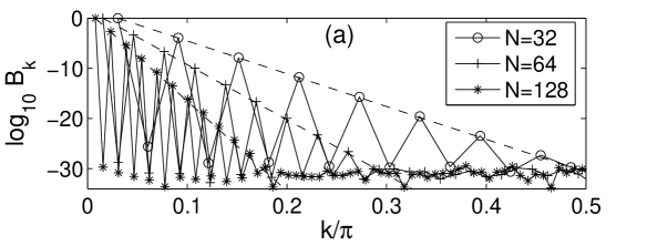
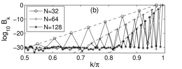
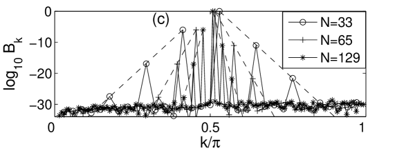
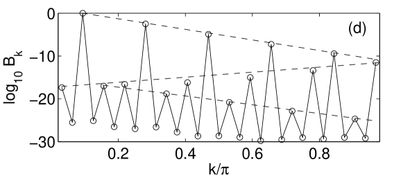
Figure 1: Distributions of mode norms for QBs in the one-dimensional DNLS model with parameters: $B=1$, $\mu=0.1$ for (a), (b), (c); (a) QBs with low-frequency seed mode $q_{0}=1$, (b) QBs with high-frequency seed mode $q_{0}=N$, (c) QBs with seed mode near the middle of the spectrum $q_{0}=1+(N+1)/2$ (c). Dashed lines in (a), (b), (c) correspond to analytical estimations. (d) Observation of multiple reflections at the boundaries of the $q$-space, $N=31$, $B=1$, $\mu=2$, $q_{0}=3$. Dashed lines in (d) are guidelines for the eye.

Let us consider the one-dimensional case. We compute $q$-breathers as the stationary solutions of the nonlinear equations (6) using the single-mode solution for $\mu=0$ as an initial approximation. Fig. 1a,b shows the distribution of mode norms for $q$-breathers in the space of wave numbers $k=\pi q/(N+1)$ for different chain sizes and different seed wave numbers, located near the lower ($k_{0}<<\pi$, Fig. 1a) and upper ($\pi-k_{0}<<\pi$, Fig. 1b) edges of the linear mode spectrum.

We find exponential localization of $q$-breathers, with a localization length which depends strongly on the chosen parameters. The obtained analytical estimations for $q$-breathers localized at the lower band edge (9),(10) respectively upper band edge (11),(12), are in quantitative agreement with numerical results (see dashed lines in Fig. 1a,b).

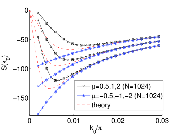
Figure 2: The slope $S$ as a function of the seed wave number $k_{0}$ for $d=1$ with fixed norm density $b=1/1025$, $\mu=\pm 0.5,\pm 1,\pm 2$ (from bottom to top). Dashed lines correspond to the analytical estimates. Different symbols: slope from the numerical calculation of QB (squares and circles represent the results for $N=512$). Solid lines guide the eye.

The exponential decay in (10) is depending on the seed mode norm density. Many applications (e.g. cold atoms in a condensate) rather fix the total norm, or total norm density. For the obtained $q$-breather solutions with $q_{0}<<N$, the relation between these quantities can be estimated by the sum of infinite geometric series:

$$B\approx\sum\limits_{n=0}^{\infty}\lambda^{n}B_{q_{0}}=\frac{B_{q_{0}}}{1-\lambda},$$ (17)

where $\lambda\equiv\lambda_{1}^{(1)}$. From (17) it follows that $b_{k_{0}}=(1-\lambda)b$, where $b=B/(N+1)$ is the total norm density. Substituting the expression for $b_{k_{0}}$ into (10) and solving the equation for $\sqrt{\lambda}$ we obtain:

$$\begin{array}[]{cc}\sqrt{\lambda}=\frac{\sqrt{1+4\nu^{4}/k_{0}^{4}}-1}{2\nu^{2}/k_{0}^{2}},&\nu^{2}=\frac{|\mu|b}{16}.\end{array}$$ (18)

The same dependence of $\sqrt{\lambda}$ on $k_{0}$ was obtained for low frequency $q$-breathers in the $\beta$-FPU model Scaling . The exponential decay of mode norms in the space of wave numbers, can be now written for $q$-breathers localized in low-frequency modes:

$$\ln b_{k}=\left(\frac{k}{k_{0}}-1\right)\ln\sqrt{\lambda}+\ln b_{k_{0}}.$$ (19)

To characterize the degree of localization in $k$-space, we use the slope of the profile of mode norms in log-normal plots (19) – $S$ Scaling , where the absolute value of $S$ is equivalent to the inverse localization length $\xi$:

$$S=\frac{1}{k_{0}}\ln\sqrt{\lambda}\;,\;|S|\equiv\xi^{-1}\;.$$ (20)

Substituting the expression for $\sqrt{\lambda}$ (18) into (20) we obtain:

$$S=\frac{1}{\nu z}\ln\left(\sqrt{1+z^{4}/4}-z^{2}/2\right)\;,\;z=k_{0}/\nu\;.$$ (21)

Therefore the slope (inverse localization length) is a function of the rescaled wavenumber $z$. It therefore parametrically depends on just one effective nonlinearity parameter $\nu$, which is given by the product of the total norm density and the absolute value of nonlinearity strength. $S$ vanishes for $z\rightarrow 0$, and it has an extremum $\min(S)\approx-0.7432/\nu$ at $z_{min}\approx 2.577$. The wave number $k_{0}=k_{min}\equiv z_{min}\nu$ corresponds to the strongest localization of a $q$-breather with fixed effective nonlinear parameter $\nu$. With increasing $\nu$ the localization length increases. Most importantly, the localization length diverges for small $k_{0}\ll k_{min}$ since $|S|\approx z/(2\nu)$ in that case. This delocalization is due to resonances with nearby normal modes close to the band edge. Note, that our analytical estimations do not depend on the sign of the nonlinearity parameter $\mu$.

In Fig. 1a,b, due to the small sizes of the chain, all values of $k_{0}$ are greater than $k_{min}$, so a monotonous dependence of the slope on $k_{0}$ is observed. In Fig. 2 we plot theoretical and numerically obtained dependencies $S(k_{0})$ for different values of the nonlinear parameter $\mu$ and different system sizes $N$ (we use large enough $N$ to resolve the theoretically predicted extremum of $S$). In all cases the numerical results show, that the slopes indeed are characterized by intensive quantities only, and the above derived scaling laws hold.

For positive values of $\mu$ and seed wave numbers close to the lower band edge, the extremum in $S$ is reproduced in the numerical data, though the numerical curves deviate from theoretical curves for small $k_{0}$. We also find that $k_{min}$ increases and $|S(k_{min})|$ decreases with increasing $\mu$ as it is predicted by our analytical results (increase of norm density $b$ gives the same effect).

For negative values of $\mu$ and seed wave numbers close to the lower band edge, we do not observe an extremum for $S$. In the region of small $k_{0}$ the numerically obtained curves for positive and negative values of $\mu$ differ, while the theoretically predicted slopes do not depend on the sign of $\mu$. Fig. 3 shows the mode norm profiles of $q$-breather solutions with small $k_{0}$ obtained for positive and negative values of $\mu$. The reason for the discrepancy between theoretical prediction and numerical results for negative values of $\mu$ must be strong contributions from higher order terms in the perturbation expansion. The standard argument is, that the perturbation theory is valid if the localization length is small, i.e. $|\lambda|\ll 1$ as well. When $|\lambda|$ becomes of the order of one, higher order terms in perturbation theory have to be taken into account, and it would be tempting to conclude that delocalization will take place. That should be true especially when all higher order terms in the series carry the same sign. That is the case for positive nonlinearity here, but for negative $\mu$ we obtain alternating signs of higher order terms. These alternating signs therefore effectively cancel most of the terms in the series, and are responsible for an increasing localization of $q$-breathers with negative $\mu$ in the limit of small wavenumbers.

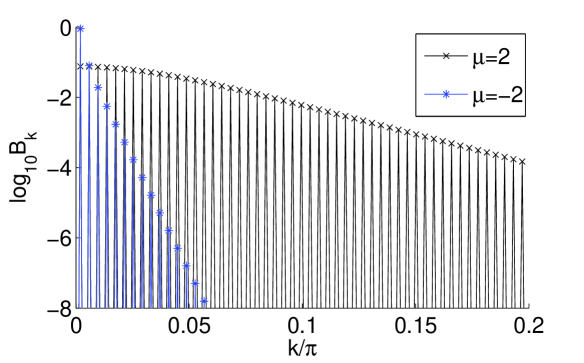
Figure 3: Distributions of mode norms for QBs in the one-dimensional DNLS model for positive and negative values of $\mu$; $q_{0}=2$, $N=1024$.

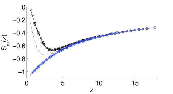
Figure 4: The master slope function $S_{m}(z)$ (dashed line). Different symbols and eye-guiding solid lines correspond to the scaled numerical estimates of the slope presented in Fig. 2 (bottom line — $\mu<0$, top line — $\mu>0$).

The obtained results for $q$-breathers with seed wave numbers close to the lower band edge ($k_{0}<<\pi$) are valid for the case of $k_{0}$ close to the upper band edge ($\pi-k_{0}<<\pi$) if we change $\mu\rightarrow-\mu$. Thus, there is a strong asymmetry in the localization properties of $q$-breather solutions with $k_{0}<\pi/2$ and $k_{0}>\pi/2$ for a fixed sign of nonlinearity.

The numerical results in Fig. 2 show that slope values calculated for different system sizes lie on the same curves with corresponding $\mu$ even in the region of small $k_{0}$, where higher order corrections to our analytical estimates have to be taken into account. This result is in agreement with the exact scaling of $q$-breather solutions described in Scaling . We plot in Fig. 4 the master slope function $S_{m}(z)=\nu S$, which depends on a single variable $z$ Scaling . It implies that knowing this single master slope function is sufficient to predict the localization property of a $q$-breather at any seed wave number $k_{0}\ll\pi$, at any energy etc. Numerically obtained slopes presented in Fig. 2 are rescaled and plotted in Fig. 4. We see, that all results corresponding to the same sign of $\mu$ condense on a single curve even (and especially) for small $k_{0}$, though these numerical results differ from the analytical estimation.

V.2 Close to the center of the band

Fig. 1c shows the distribution of mode norms for $q$-breathers in the space of wave numbers $k=\pi q/(N+1)$ for different chain sizes and different seed wave numbers, located close to the center of the spectrum ($|k_{0}-\pi/2|<<\pi$). The analytical estimation for the amplitudes of these $q$-breathers are in good quantitative agreement with the numerical results, for small enough parameters $\mu$ and $b$, cf. Fig. 1c.

We express again the norm density of the seed mode via the total norm density: $b_{k_{0}}=(1-\lambda)b$, ($\lambda\equiv\lambda_{1}^{(1)}$). Substituting this expression into (14) we find:

$$\begin{array}[]{cc}\sqrt{\lambda}=\frac{\sqrt{1+4\nu^{2}/(k_{0}-\pi/2)^{2}}-1}{2\nu/|k_{0}-\pi/2|},&\nu=\frac{|\mu|b}{8}.\end{array}$$ (22)

The slope of the mode norm profile in $k$-space is given by

$$S=\frac{1}{|k_{0}-\pi/2|}\ln\sqrt{\lambda}=\frac{1}{2\nu z}\ln\left(\sqrt{1+z^{2}}-z\right),$$ (23)

where $z=|k_{0}-\pi/2|/(2\nu)$. For $z<<1$: $S=(-1+z^{2}/6+O(z^{4}))/(2\nu)$, for $z>>1$: $S=\ln(1/(2z)+O(1/z^{3}))/(2\nu z)$. In the limit $z\rightarrow 0$, the slope $S\rightarrow-1/(2\nu)$. Thus, the strongest localization of a $q$-breather with fixed effective nonlinear parameter $\nu$ should be obtained for wave numbers $k_{0}\approx\pi/2$. The increase of the effective nonlinearity parameter $\nu\sim|\mu|b$ leads to a weaker localization of $q$-breathers in $k$-space, since the absolute value of the slope $S$ decreases. Note, that there is a special point for odd $N$: $k_{0}=\pi/2$, $q_{0}=(N+1)/2$. For this seed mode, the $q$-breather is compact in $k$-space SPO .

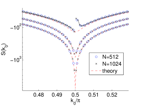
Figure 5: The slope $S$ as a function of the seed wave number $k_{0}$ for $d=1$ with fixed norm density $b=1/1025$, $\mu=0.5,5,30$ (from bottom to top). Dashed lines correspond to the analytical estimates. Different symbols correspond to the estimates of the slopes from numerical calculations of QBs.

In Fig. 5 the theoretical and numerically obtained dependencies $S(k_{0})$ for different values of $\mu$ and different system sizes $N$ are plotted. For small values of $\mu$ we observe good agreement between analytical and numerical results. But the increase of the nonlinearity leads to a deviation between the theoretical and numerical curves in the region of $k_{0}$ close to $\pi/2$. These corrections, as it was for the case of $q$-breathers localized near the band edges, depend on the location of $k_{0}$ ($k_{0}>\pi/2$ or $k_{0}<\pi/2$) and on the sign of nonlinearity. Therefore the curves of $S(k_{0})$ for strong nonlinearity ($\mu=30$) in Fig. 5 are non-symmetric around the point $k_{0}=\pi/2$: in contrast to $k_{0}<\pi/2$, for $k_{0}>\pi/2$ a local minimum of $S$ is observed. Still, the predicted scaling properties of $q$-breathers remain correct even for strong nonlinearity: the values of $S$, computed for different system sizes $N$, lie on the same curves for fixed $\mu$.

V.3 Stability of $q$-breathers

We analyze the linear stability of $q$-breathers as stationary solutions of DNLS model considering the evolution of small perturbations $\varepsilon_{n}$ in the rotating frame of the periodic solution Gorbach : $\psi_{\boldsymbol{n}}(t)=(\phi_{\boldsymbol{n}}^{0}+\varepsilon_{\boldsymbol{n}}(t))\exp(i\Omega t)$, where $\phi_{\boldsymbol{n}}^{0}$ are the non-perturbed time-independent amplitudes, $\varepsilon_{\boldsymbol{n}}=\alpha_{\boldsymbol{n}}+i\beta_{\boldsymbol{n}}$. A periodic orbit is stable when all perturbations do not grow in time. Solving the linearized equations for the perturbation, that condition translates into the request, that all eigenvalues $s_{m}$ ($m=\overline{1,2N^{d}}$) of the linearized equations must be purely imaginary. Otherwise the orbit is unstable.

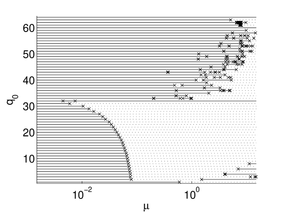
Figure 6: Domain of stability of $q$-breathers for $d=1$. Solid lines - stable, dashed - unstable, crosses - switch from stable to unstable or vice versa. $N=64$, $B=2$.

In Fig. 6 we plot the numerical outcome of the stability analysis. We smoothly continue $q$-breather solutions for each seed mode number $q_{0}$ by increasing the nonlinearity parameter $\mu$ and check the stability. If the maximum absolute value of the real parts of all eigenvalues is smaller than $10^{-6}$, the $q$-breather is considered as stable (solid line), otherwise it is unstable (dashed line), crosses mark the change of stability. For small values of nonlinearity all $q$-breathers are stable. Qualitatively different threshold values and dependencies on $q_{0}$ for $q$-breathers with seed modes from different parts of the spectrum $q_{0}<N/2$ and $q_{0}>N/2$ are observed. This is in agreement with the results presented in SW , where stability properties of nonlinear standing waves are studied. Note, that due to the symmetry of the equations, the stability properties of a $q$-breather with seed mode $q_{0}$ for some negative value of the nonlinearity parameter $\mu$ is the same as the stability property of the $q$-breather with seed mode $\widetilde{q}_{0}=N+1-q$ for the nonlinearity parameter $\widetilde{\mu}=-\mu$.

Let us discuss the possible link between linear stability and localization. If a $q$-breather becomes delocalized, that happens because of resonances between different mode frequencies. Therefore we can expect, that the same resonances will also drive the state unstable. Indeed, these correlations can be clearly observed from the numerical data. However, if a $q$-breather is well localized, it does not follow that it will be stable as well, since instability can arise due to resonant interaction of modes in the breather core alone.

VI Periodic boundary conditions

In the case of periodic boundary conditions, we have used the following transformations between real space and the reciprocal space of normal modes (for even $N$):

$$\begin{array}[]{l}\psi_{\boldsymbol{n}}(t)=\frac{1}{N^{d/2}}\sum\limits_{q_{1},\ldots,q_{d}=-N/2+1}^{N/2}Q_{\boldsymbol{q}}(t)\prod\limits_{i=1}^{d}\exp{\left(\frac{2\pi q_{i}(n_{i}-1)}{N}\right)}\;.\end{array}$$ (24)

The DNLS model (1) with periodic boundary conditions has exact solutions for nonlinear traveling waves, which can be written, for instance in case $d=1$, as: $\psi_{n}(t)=\phi_{0}\exp(i\Omega t-ik_{0}n)$, where $\Omega=-2\cos k_{0}-\mu\phi_{0}^{2}$, $k_{0}=2\pi q_{0}/N$, $q_{0}\in[-N/2,N/2]$. These types of solutions can be considered as compact $q$-breathers which contain only one mode $q_{0}$. Traveling modes are also not invariant under time reversal.

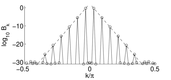
Figure 7: Time-reversible $q$-breather in the one-dimensional DNLS model with periodic boundary conditions, continued from the linear standing wave consisting of two traveling waves with $q_{0}=2$ and $q_{0}=-2$, $N=64$, $B=1$, $\mu=0.1$. Dashed lines represent analytical estimations.

The continuation of a linear standing wave, consisting of two traveling waves with the same norms and wave numbers: $k_{0}$ and $-k_{0}$, into the nonlinear regime leads to a time-reversible $q$-breather solution (see Fig. 7), which is not compact, and its localization properties are similar to the properties of $q$-breathers in the case of fixed boundary conditions. Here we present the result for decay of mode norms $\lambda_{d}^{(i)}$ for the case $|k_{i,0}|<<\pi$, which differs from (10) by a prefactor:

$$\begin{array}[]{cc}\sqrt{(\lambda_{d}^{(i)})}=\frac{|\mu|A_{\boldsymbol{q}_{0}}^{2}N^{2-d}}{32\pi^{2}{(q_{i,0})}^{2}}=\frac{|\mu|b_{\boldsymbol{k}_{0}}}{8{(k_{i,0})}^{2}}\;,&i=\overline{1,d}\;,\end{array}$$ (25)

where $b_{\boldsymbol{k}_{0}}=B_{\boldsymbol{k}_{0}}/N^{d}$, $k_{i,0}=2\pi q_{i,0}/N$. Fig. 7 illustrates good quantitative agreement between analytical and numerical results obtained for small enough values of norm and nonlinearity.

VII $q$-breathers in two- and three-dimensional lattices

For two- and three-dimensional symmetric DNLS lattices (1) with fixed boundary conditions, only linear modes with mode numbers $\boldsymbol{q}$ on the main diagonal have non-degenerate frequencies. Using the Implicit Function Theorem ImpFunc , it follows that these modes are continued into the nonlinear regime. However, we also successfully performed numerical continuations of $q$-breathers with seed mode numbers off the main diagonal as it was done in FPU2d3d for the FPU model. For the two-dimensional DNLS model the $q$-breather, continued from the single linear mode $\boldsymbol{q}_{0}=(2,3)$, is presented in Fig. 8 in real space (a) and in $q$-space (b). The $q$-breather with the seed mode $\boldsymbol{q}_{0}=(3,2)$ exists as well and has the same frequency. The slowest decay of the mode norms happens to be along the direction of the main axes. The decay is exponential and in good agreement with the analytical estimation (10) for $d=2$.

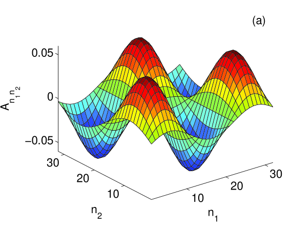
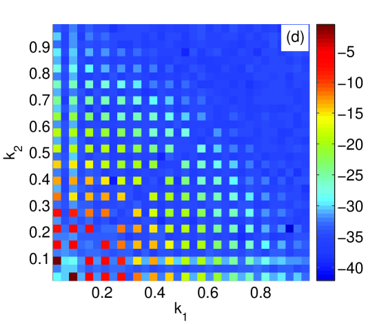
Figure 8: Different $q$-breather modes for $d=2$: $N=32$, $B=1$, $\mu=0.5$. Mode norm magnitude is plotted in color code on logarithmic scale (except for (a), where a linear scale is used). (a), (b) — asymmetric single-mode $q$-breather with seed mode ($\boldsymbol{q}_{0}=(3,2)$) in real space (a) and in $q$-space (b); (c), (d) — symmetric multi-mode $q$-breather with in-phase (c) and antiphase (d) seed mode pair $\boldsymbol{q}=(3,1),(1,3)$. Dashed line in (b) guides the eye along the main diagonal.

In addition to such asymmetric single mode $q$-breathers it is possible to construct multi-mode $q$-breathers continued from a pair of degenerate linear normal modes $(q_{0},p_{0})$ and $(p_{0},q_{0})$ ($q_{0}\neq p_{0}$) with the same norms in both modes and in-phase (Fig. 8c) or antiphase (Fig. 8d) oscillations. It is important to note that the problem of degenerate frequencies is avoided for these solutions. Indeed, system (4) has two invariant manifolds $Q_{q_{1},q_{2}}=\pm Q_{q_{2},q_{1}}$. Looking for a solution on a manifold, the number of independent variables of state is reduced from $N^{2}$ to the dimensionality of the manifold, which equals $(N^{2}+N)/2$ for the symmetric manifold and $(N^{2}-N)/2$ for the antisymmetric one. The reduced system of equations contains only modes with non-degenerate frequencies.

For $d=3$ we have also verified, that the analytical estimations of mode norm decay (10), (14) agree well with the results of numerical calculations for single-mode $q$-breathers.

In addition to various time-reversible $q$-breather solutions, which are constructed in the same way as for $d=2$, the three-dimensional DNLS model allows also for non-time-reversible (“vortex”) multi-mode solutions. Let us consider $q$-breather solutions on an invariant manifold of the system (4): $Q_{q_{1},q_{2},q_{3}}=\exp(2\pi i/3)Q_{q_{3},q_{1},q_{2}}=\exp(4\pi i/3)Q_{q_{2},q_{3},q_{1}}$ (note, that this manifold has a counterpart with the opposite sign of the phase shifts). On the manifold the number of variables of state is reduced to $(N^{3}-N)/3$. We have constructed numerically a vortex $q$-breather solution continued from a degenerate triplet of seed modes which have the same norm and a relative phase shift $2\pi/3$: $Q_{q_{0},q_{0},p_{0}}=\exp(2\pi i/3)Q_{p_{0},q_{0},q_{0}}=\exp(4\pi i/3)Q_{q_{0},p_{0},q_{0}}$, $q_{0}\neq p_{0}$. The frequency of such a triplet becomes non-degenerate in the reduced system on the manifold. The energy flows in a vortex-like manner in $q$-space for such excitations (Fig.9).

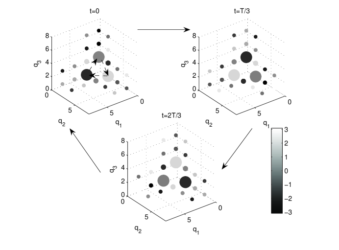
Figure 9: A vortex $q$-breather state for $d=3$: $N=8$, $B=1$, $\mu=0.1$, at some fixed time. Mode norm magnitude is encoded in sphere sizes on logarithmic scale, while the sphere color denotes the phase of the mode. Seed mode triplet: $\boldsymbol{q}=(3,1,1),(1,3,1),(1,1,3)$.

VIII Discussion

Comparing the aims we formulated in the introduction with the above results, we can conclude, that indeed the $q$-breather concept turns out to be generic, and time-periodic orbits, which are localized in normal mode space, are probably as generic as discrete breathers (although perhaps in a different way). Along with the study of the details of $q$-breathers properties in DNLS models, we found some particularities, which were not (yet) obtained in acoustic (FPU) systems. Let us discuss some of these and other findings from above.

VIII.1 Scales, delocalization thresholds, and healing length of a BEC

Let us consider a finite DNLS chain with $N$ sites. Let us fix the total norm density $b$ and the nonlinearity $\mu$. Therefore we fix the effective nonlinearity parameter $\nu^{2}=|\mu|b/16$ (18). If the system size was large enough, we will resolve the extremum in $S$, and therefore the QB with seed wave number $k_{min}\approx 2.577\nu$ is the strongest localized one. It evidently sets an inverse length scale $\nu$. This length scale is known in the GP equation for a BEC in a trap with (similar) fixed boundary conditions. One has a condensate, whose amplitude vanishes at some boundary, yet getting back to some mean value away from the boundary - exactly at the healing length $\xi_{h}=(4\pi an)^{-1/2}$, where $n$ is the condensate density, and $a$ is the scattering length which is proportional to the atom-atom interaction, and therefore to the nonlinearity strength $\mu$ within the mean field GP equation healinglength . Therefore, the inverse healing length corresponds to the wave number scale, on which the most strongly localized QB is observed.

We now increase the system size further, and compute the localization length (or respectively its negative inverse - the slope $S$) of the longest wavelength mode. With increasing $N$ the grid of allowed $k$-values becomes denser, and at some critical $N_{c}(\nu)$ the localization length will reach the finite size of the normal mode space, and the $q$-breather delocalizes. With a little algebra it follows

$$N_{c}\approx\frac{\pi^{2}}{2\nu^{2}}\;,\;k_{0}^{(c)}\approx\frac{2\nu^{2}}{\pi}\;.$$ (26)

For even larger (and finally infinitely large) lattices the critical value $k_{0}^{(c)}$ is marking a border in $k$-space: at the given norm density $\nu$, all QBs with seed wave numbers $k\gg k_{0}^{(c)}$ are localized, while we obtain delocalization for $k\leq k_{0}^{(c)}$. So there is a layer of delocalized QBs at the band edge, whose width grows according to (26) with growing $\nu$. Modes launched inside this layer (with the given norm density) will quickly spread their energy among many other modes - they will quickly relax. Modes launched outside this layer will stay localized in normal mode space, at least for sufficiently long times. $k_{0}^{(c)}$ is therefore separating a layer of strongly interacting modes from weakly interacting ones. For large enough effective nonlinearity parameter $\nu\sim 1$ the whole wave number space is filled with strongly interacting normal modes, and the normal mode picture breaks down completely. As long as $\nu$ is smaller, the value of $k_{0}^{(c)}$ sets a new length scale $2\pi/k_{0}^{(c)}$, which is proportional to the squared healing length $\xi_{h}^{2}$. On that new length scale, the normal mode picture breaks down.

VIII.2 Delocalization thresholds and modulational instability

It is instructive to remember, that delocalization thresholds of QBs are related to resonances. Indeed, in the present case, the density of states at the band edge diverges in the limit of large system size, and many modes have almost the same frequencies. It is these small differences, which tend to zero as $1/N^{2}$, and which are responsible for the resonant mode-mode interaction. Notably the analysis of stability of band edge modes bem (note: for periodic boundary conditions) shows some interesting correlations. The analyzed band edge modes are compact in normal mode space, yet they undergo a tangent bifurcation at amplitudes, which are the smaller, the larger the system size. These instabilities appear however only for a certain sign of the nonlinearity, which exactly corresponds to the actual observed delocalization of QBs. Therefore we expect, that the (so far not studied) case of a FPU chain with negative quartic nonlinearity, which is known not to yield an instability for the band edge mode, will not show delocalization of QBs close to the (upper) band edge. It is furthermore instructive, that if a tangent bifurcation of a band edge mode takes place, the simulation of a lattice shows the onset of modulational instability, which leads to a collection of energy in smaller system volumes, and finally to the formation of discrete breathers - i.e. to localization in real space. Thus we may expect, that the resonant layer of strongly interacting modes may lead to the formation of localized states in real space, while the rest of the normal mode space is evolving in the regime of localization in normal mode space. Thus, we may expect to observe in an actual simulation localization both in normal mode space and in real space.

VIII.3 Comparing analytical and numerical results

While the delocalization at one band edge, as predicted by perturbation theory, is reproduced by numerical data, that does not happen at the second band edge (both band edges change their places, when the nonlinearity inverts sign). The breakdown of perturbation theory follows from comparing the leading and next-to-leading order terms in the expansion. When terms are of the same order, we conclude, that the series will diverge, and therefore the QB solutions will delocalize. This is true for the case when all terms in the series have the same sign. However, when the terms have alternating sign, the above conclusion must not be correct. And indeed the numerical data show, that these sign alternations lead to an effective cancelation, and a final strong localization of a QB solution. A similar breakdown of perturbation theory happens for QB solutions localized at the band center for large nonlinearity (or norm). The perturbation theory tells, that QB states are well localized from both sides of the center. Numerical data however show, that this is true only on one side from the center, while the other side shows a tendency towards delocalization.

VIII.4 Open questions

Below we list some potentially interesting and important open questions. First, the influence of different boundary conditions has not been systematically studied. QBs are extended states in real space, therefore their spectrum, and the way they interact, may to some extend be sensitive to the choice of boundary conditions.

Second, it remains completely open, what kind of excitation we catch by considering a vortex state in normal mode space.

Finally, it would be interesting to see the changes in the QB properties, when the norm conservation is lifted. In general we expect, that this will lead to the generation of higher harmonics, and new types of resonances. In fact it is exactly resonances due to higher harmonics, which give the leading order contribution to the FPU problem. However, for sufficiently narrow optical bands, higher harmonics will be located outside the optical band. These resonances will be therefore important, when the optical band is wide, or when one considers a complex and broader band structure.

Acknowledgements
Part of this work was completed while SF was visiting the Institute for Mathematical Sciences, National University of Singapore in 2007. KM, OK and MI acknowledge support from RFBR, grants No. 06-02-16499, 07-02-01404.

References

- (1) E. Fermi, J. Pasta, and S. Ulam, Los Alamos Report LA-1940, (1955); also in: Collected Papers of Enrico Fermi, ed. E. Segre, Vol. II (University of Chicago Press, 1965) p.977-978; Many-Body Problems, ed. D. C. Mattis (World Scientific, Singapore, 1993)
- (2) L. Galgani and A. Scotti, Phys. Rev. Lett. 28, 1173 (1972).
- (3) L. Berchialla, A. Giorgilli and S. Paleari, Phys. Lett. A 321 167 (2004).
- (4) F. M. Izrailev and B. V. Chirikov, Sov. Phys. Dokl. 11, 30 (1966).
- (5) N. J. Zabusky and M. D. Kruskal, Phys. Rev. Lett. 15, 240 (1965).
- (6) J. De Luca, A. Lichtenberg and M. A. Lieberman, Chaos 5, 283 (1995).
- (7) J. Ford, Phys. Rep. 213, 271 (1992); Focus issue, The Fermi-Pasta-Ulam Problem - The First Fifty Years, edited by D. K. Campbell, P. Rosenau and G. M. Zaslavsky, Chaos 15 No. 1 (2005).
- (8) A. J. Sievers and S. Takeno, Phys. Rev. Lett. 61, 970 (1988); T. Dauxois, M. Peyrard and C. R. Willis, Physica D 57, 267 (1992); S. Flach and C. R. Willis, Phys. Lett. A 181, 232 (1993).
- (9) A. A. Ovchinnikov, Sov. Phys. JETP 57, 147 (1970).
- (10) R. S. MacKay and S. Aubry, Nonlinearity 7, 1623 (1994); S. Aubry, Physica D 103, 201 (1997); S. Flach and C. R. Willis, Phys. Rep. 295, 192 (1998); T. Dauxois, A. Litvak-Hinenzon, R. S. MacKay and A. Spanoudaki (Eds), Energy localization and transfer, World Scientific, Singapore (2004); S. Flach and A. V. Gorbach, submitted to Phys. Rep. (2007).
- (11) S. Flach, M. V. Ivanchenko and O. I. Kanakov, Phys. Rev. Lett. 95, 064102 (2005); S. Flach, M. V. Ivanchenko and O. I. Kanakov, Phys. Rev. E 73 036618 (2006); T. Penati and S. Flach, Chaos 17, 023102 (2007); S. Flach and A. Ponno, Physica D, in print, arXiv 0705.0804 [nlin.PS] (2007).
- (12) M.V. Ivanchenko, O.I. Kanakov, K.G. Mishagin, and S. Flach, Phys. Rev. Lett. 97 025505 (2006).
- (13) O.I. Kanakov, S.Flach, M.V. Ivanchenko, and K.G. Mishagin, Phys. Lett. A 365, 416 (2007); S. Flach, O.I. Kanakov, K.G. Mishagin and M.V. Ivanchenko, Int. J. of Modern Phys. B 21, 3925 (2007).
- (14) Y. S. Kivshar and M. Peyrard, Phys. Rev. A 46, 3198 (1992); M. Johansson, Physica D 216, 62 (2006).
- (15) L. P. Pitaevskii, Sov. Phys. JETP 13, 451 (1961); E. P. Gross, Nuovo Cimento 20, 454 (1961).
- (16) O. Morsch and M. Oberthaler, Rev. Mod. Phys. 78, 179 (2006).
- (17) Yu. S. Kivshar and G. P. Agrawal, Optical solitons: from fibers to photonic crystals, Elsevier Science, Amsterdam (2003).
- (18) J. Dieudonne, Foundations of modern analysis, Academic, New York (1969).
- (19) -breathers with seed linear modes ,, () are compact in -space because these seed modes do not excite the other modes due to the selection rules (5).
- (20) R. L. Bivins, N. Metropolis and J. R. Pasta, J. Comput. Phys. 12, 65 (1973); G. M. Chechin, N. V. Novikova and A. A. Abramenko, Physica D 166, 208 (2002); B. Rink, Physica D 175, 31 (2002).
- (21) A.A. Morgante, M. Johansson, G. Kopidakis, and S. Aubry, Physica D, 162, 53 (2002); M. Johansson, A.M. Morgante, S. Aubry, and G. Kopidakis, Eur. Phys. J. B 29, 279 283 (2002)
- (22) A.V. Gorbach and M. Johansson, Eur. Phys. J. D, 29, 77 (2004).
- (23) N. Budinsky and T. Bountis, Physica D8, 445 (1983); K. W. Sandusky and K. B. Page, Phys. Rev. B 50, 866 (1994); S. Flach, Physica D 91, 223 (1996); J. Dorignac and S. Flach, Physica D 204, 83 (2005).