Simulation techniques for cosmological simulations

Abstract

Modern cosmological observations allow us to study in great detail the evolution and history of the large scale structure hierarchy. The fundamental problem of accurate constraints on the cosmological parameters, within a given cosmological model, requires precise modelling of the observed structure. In this paper we briefly review the current most effective techniques of large scale structure simulations, emphasising both their advantages and shortcomings. Starting with basics of the direct N-body simulations appropriate to modelling cold dark matter evolution, we then discuss the direct-sum technique GRAPE, particle-mesh (PM) and hybrid methods, combining the PM and the tree algorithms. Simulations of baryonic matter in the Universe often use hydrodynamic codes based on both particle methods that discretise mass, and grid-based methods. We briefly describe Eulerian grid methods, and also some variants of Lagrangian smoothed particle hydrodynamics (SPH) methods.

1 Introduction

In the hierarchical picture of structure formation, small objects collapse first and then merge to form larger and larger structures in a complex manner. This formation process reflects on the intricate structure of galaxy clusters, whose properties depend on how the thousands of smaller objects that the cluster accretes are destroyed or survive within the cluster gravitational potential. These merging events are the source of shocks, turbulence and acceleration of relativistic particles in the intracluster medium, which, in turn, lead to a redistribution or amplification of magnetic fields, and to the acceleration of cosmic rays. In order to model these processes realistically, we need to resort to numerical simulations which are capable of resolving and following correctly the highly non-linear dynamics. In this paper, we briefly describe the methods which are commonly used to simulate galaxy clusters within a cosmological context.

Usually, choosing the simulation setup is a compromise between the size of the region that one has to simulate to fairly represent the object(s) of interest, and the resolution needed to resolve the objects at the required level of detail. Typical sizes of the simulated volume are a megaparsec scale for an individual galaxy, tens to hundreds of megaparsecs for a galaxy population, and several hundreds of megaparsecs for a galaxy cluster population. The mass resolution varies from $\approx 10^{5}$ M_⊙ up to $\approx 10^{10}$ M_⊙, depending on the object studied, while, nowadays, one can typically reach the resolution of a few hundred parsec for individual galaxies and above the kiloparsec scale for cosmological boxes.

2 N-Body (pure gravity)

Over most of the cosmic time of interest for structure formation, the Universe is dominated by dark matter. The most favourable model turned out to be the so-called cold dark matter (CDM) model. The CDM can be described as a collisionless, non-relativistic fluid of particles of mass $m$, position ${\bf{x}}$ and momentum ${\bf{p}}$. In an expanding background Universe (usually described by a Friedmann-Lemaître model), with $a=(1+z)^{-1}$ being the Universe scale factor, ${\bf{x}}$ is the comoving position and the phase-space distribution function $f({\bf{x}},{\bf{p}},t)$ of the dark-matter fluid can be described by the collisionless Boltzmann (or Vlasov) equation

$$\frac{\partial f}{\partial t}+\frac{{\bf{p}}}{ma^{2}}{\bf{\nabla}}f-m{\bf{\nabla}}\Phi\frac{\partial f}{\partial{\bf{p}}}=0$$ (1)

coupled with the Poisson equation

$${\bf{\nabla}}^{2}\Phi({\bf{x}},t)=4\pi{\rm G}a^{2}\left[\rho({\bf{x}},t)-\bar{\rho}(t)\right],$$ (2)

where $\Phi$ is the gravitational potential and $\bar{\rho}(t)$ is the background density. The proper mass density

$$\rho({\bf{x}},t)=\int{f({\bf{x}},{\bf{p}},t)\mathrm{d}^{3}p}$$ (3)

can be inferred by integrating the distribution function over the momenta ${\bf{p}}=ma^{2}\dot{{\bf{x}}}$.

This set of equations represents a high-dimensional problem. It is therefore usually solved by sampling the phase-space density by a finite number $N$ of tracer particles. The solution can be found through the equation of motion of the particles (in comoving coordinates),

$$\frac{\mathrm{d}{\bf{p}}}{\mathrm{d}t}=-m{\bf{\nabla}}\Phi$$ (4)

and

$$\frac{\mathrm{d}{\bf{x}}}{\mathrm{d}t}=\frac{{\bf{p}}}{ma^{2}}.$$ (5)

Introducing the proper peculiar velocity ${\bf{v}}=a\dot{{\bf{x}}}$ these equations can be written as

$$\frac{\mathrm{d}{\bf{v}}}{\mathrm{d}t}+{\bf{v}}\frac{\dot{a}}{a}=-\frac{{\bf{\nabla}}\Phi}{a}.$$ (6)

The time derivative of the expansion parameter, $\dot{a}$, can be obtained from the Friedmann equation

$$\dot{a}=H_{0}\sqrt{1+\Omega_{0}(a^{-1}-1)+\Omega_{\Lambda}(a^{2}-1)},$$ (7)

where we have assumed the dark energy to be equivalent to a cosmological constant. For a more detailed description of the underlying cosmology and related issues, see for example Peebles (1980) or others.

There are different approaches: to solve directly the motion of the tracer particles, or to solve the Poisson equation. Some of the most common methods will be described briefly in the following sections.

2.1 Direct sum (GRAPE, GPU)

The most direct way to solve the N-body problem is to sum directly the contributions of all the individual particles to the gravitational potential

$$\Phi({\bf{r}})=-{\rm G}\sum_{j}\frac{m_{j}}{\left(|{\bf{r}}-{\bf{r}}_{j}|^{2}+\epsilon^{2}\right)^{\frac{1}{2}}}.$$ (8)

In principle, this sum would represent the exact (Newtonian) potential which generates the particles’ acceleration. As mentioned before, the particles do not represent individual dark matter particles, but should be considered as Monte Carlo realisations of the mass distribution, and therefore only collective, statistical properties can be considered. In such simulations, close encounters between individual particles are irrelevant to the physical problem under consideration, and the gravitational force between two particles is smoothed by introducing the gravitational softening $\epsilon$. This softening reduces the spurious two-body relaxation which occurs when the number of particles in the simulation is not large enough to represent correctly a collisionless fluid. This situation however is unavoidable, because the number of dark matter particles in real systems is orders of magnitude larger than the number that can be handled in a numerical simulation. Typically, $\epsilon$ is chosen to be $1/20-1/50$ of the mean inter-particle separation within the simulation. In general, this direct-sum approach is considered to be the most accurate technique, and is used for problems where superior precision is needed. However this method has the disadvantage of being already quite CPU intensive for even a moderate number of particles, because the computing time is $\propto N^{2}$, where $N$ is the total number of particles.

Rather than searching for other software solutions, an alternative approach to solve the $N^{2}$-bottleneck of the direct-sum technique is the GRAPE (GRAvity PipE) special-purpose hardware (see e.g. Ito et al. 1993 and related articles). This hardware is based on custom chips that compute the gravitational force with a hardwired Plummer force law (Eq. 8). This hardware device thus solves the gravitational N-body problem with a direct summation approach at a computational speed which is considerably higher than that of traditional processors.

For the force computation, the particle coordinates are first loaded onto the GRAPE board, then the forces for several positions (depending on the number of individual GRAPE chips installed in the system) are computed in parallel. In practice, there are some technical complications when using the GRAPE system. One is that the hardware works internally with special fixed-point formats or with limited floating point precision (depending on the version of the GRAPE chips used) for positions, accelerations and masses. This results in a reduced dynamic range compared to the standard IEEE floating point arithmetic. Furthermore, the communication time between the host computer and the GRAPE system can be an issue in certain circumstances. However, newer versions of the GRAPE chips circumvent this problem, and can also be combined with the tree algorithms (which are described in detail in the next section), see Fukushige et al. (1991); Makino (1991); Athanassoula et al. (1998); Kawai et al. (2000).

By contrast, the graphic processing unit (GPU) on modern graphic cards now provides an alternative tool for high-performance computing. The original purpose of the GPU is to serve as a graphics accelerator for speeding up the image processing, thereby allowing one to perform simple instructions on multiple data. It has therefore become an active area of research to use the GPUs of the individual members of computer clusters. Although very specialised, many of those computational algorithms are also needed in computational astrophysics, and therefore the GPU can provide significantly more computing power than the host system; thereby providing a high performance with typically large memory size and at relatively low cost, which represents a valid alternative to special purpose hardware like GRAPE. For recent applications to astrophysical problems see Schive et al. (2007) and references therein.

2.2 Tree

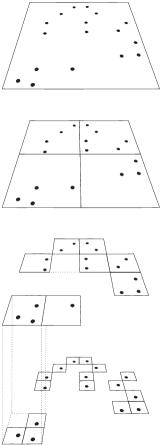
Figure 1: Schematic illustration of the Barnes & Hut (1986) oct-tree in two dimensions. The particles are first enclosed in a square (root node). This square is then iteratively subdivided into four squares of half the size, until exactly one particle is left in each final square (leaves of the tree). In the resulting tree structure, each square can be the progenitor of up to four siblings. Taken from Springel et al. (2001b).

The primary method of solving the N-body problem is a hierarchical multipole expansion, commonly called a tree algorithm. This method groups distant particles into larger cells, allowing their gravity to be accounted for by means of a single multipole force. Instead of requiring $N-1$ partial force evaluations per particle, as needed in a direct-summation approach, the gravitational force on a single particle can be computed with substantially fewer operations, because distant groups are treated as “macro” particles in the sum. In this manner the sum usually reduces to $N\mathrm{log}(N)$ operations. Note however that this scaling is only true for homogeneous particle distributions, whereas the scaling for strongly inhomogeneous distributions, as present in evolved cosmological structures, can be less efficient.

In practice, the hierarchical grouping that forms the basis of the multipole expansion is most commonly obtained by a recursive subdivision of space. In the approach of Barnes & Hut (1986), a cubical root node is used to encompass the full mass distribution; the cube is repeatedly subdivided into eight daughter nodes of half the side-length each, until one ends up with ‘leaf’ nodes containing single particles (see Fig. 1). Forces are then obtained by “walking” the tree. In other words, starting at the root node, a decision is made as to whether or not the multipole expansion of the node provides an accurate enough partial force. If the answer is ‘yes’, the multipole force is used and the walk along this branch of the tree can be terminated; if the answer is ‘no’, the node is “opened”, i.e. its daughter nodes are considered in turn. Clearly, the multipole expansion is in general appropriate for nodes that are sufficiently small and distant. Most commonly one uses a fixed angle (typically $\approx 0.5$ rad) as opening criteria.

It should be noted that the final result of the tree algorithm will in general only represent an approximation to the true force. However, the error can be controlled conveniently by modifying the opening criterion for tree nodes, because a higher accuracy is obtained by walking the tree to lower levels. Provided that sufficient computational resources are invested, the tree force can then be made arbitrarily close to the well-specified correct force. Nevertheless evaluating the gravitational force via a tree leads to an inherent asymmetry in the interaction between two particles. It is worth mentioning that there are extensions to the standard tree, the so-called fast multipole methods, which avoid these asymmetries, and therefore have better conservation of momentum. For an N-body application of such a technique see Dehnen (2000) and references therein. However, these methods compute the forces for all the particles at every time step and can not take advantage of using individual time steps for different particles.

2.3 Particle-Mesh methods

The Particle-Mesh (PM) method treats the force as a field quantity by computing it on a mesh. Differential operators, such as the Laplacian, are replaced by finite difference approximations. Potentials and forces at particle positions are obtained by interpolation on the array of mesh-defined values. Typically, such an algorithm is performed in three steps. First, the density on the mesh points is computed by assigning densities to the mesh from the particle positions. Second, the density field is transformed to Fourier space, where the Poisson equation is solved, and the potential is obtained using Green’s method. Alternatively, the potential can be determined by solving Poisson’s equation iteratively with relaxation methods. In a third step the forces for the individual particles are obtained by interpolating the derivatives of the potentials to the particle positions. Typically, the amount of mesh cells $N$ used corresponds to the number of particles in the simulation, so that when structures form, one can have large numbers of particles within individual mesh cells, which immediately illustrates the shortcoming of this method; namely its limited resolution. On the other hand, the calculation of the Fourier transform via a Fast Fourier Transform (FFT) is extremely fast, as it only needs of order $N\log N$ operations, which is the advantage of this method. Note that here $N$ denotes the number of mesh cells. In this approach the computational costs do not depend on the details of the particle distribution. Also this method can not take advantage of individual time steps, as the forces are always calculated for all particles at every time step.

There are many schemes to assign the mass density to the mesh. The simplest method is the “Nearest-Grid-Point” (NGP). Here, each particle is assigned to the closest mesh point, and the density at each mesh point is the total mass assigned to the point divided by the cell volume. However, this method is rarely used. One of its drawbacks is that it gives forces that are discontinuous. The “Cloud-in-a-Cell” (CIC) scheme is a better approximation to the force: it distributes every particle over the nearest 8 grid cells, and then weighs them by the overlapping volume, which is obtained by assuming the particle to have a cubic shape of the same volume as the mesh cells. The CIC method gives continuous forces, but discontinuous first derivatives of the forces. A more accurate scheme is the “Triangular-Shaped-Cloud” (TSC) method. This scheme has an assignment interpolation function that is piecewise quadratic. In three dimensions it employs 27 mesh points (see Hockney & Eastwood 1988).

In general, one can define the assignment of the density $\rho_{m}$ on a grid ${\bf{x}}_{m}$ with spacing $\delta$ from the distribution of particles with masses $m_{i}$ and positions ${\bf{x}}_{i}$, by smoothing the particles over $n$ times the grid spacing ($h=n\delta$). Therefore, having defined a weighting function

$$W({\bf{x}}_{m}-{\bf{x}}_{i})=\int\hat{W}\left(\frac{{\bf{x}}-{\bf{x}_{m}}}{h}\right)\,S({\bf{x}}-{\bf{x}_{i}},h)\mathrm{d}{\bf{x}},$$ (9)

where $\hat{W}({\bf{x}})$ is $1$ for $|{\bf{x}}|<0.5$ and $0$ otherwise, the density $\rho_{m}$ on the grid can be written as

$$\rho_{m}=\frac{1}{h^{3}}\sum_{i}m_{i}W({\bf{x}}_{i}-{\bf{x}}_{m}).$$ (10)

The shape function $S({\bf{x}},h)$ then defines the different schemes. The aforementioned NGP, CIC and TSC schemes are equivalent to the choice of 1, 2 or 3 for $n$ and the Dirac $\delta$ function $\delta({\bf{x}})$, $\hat{W}({\bf{x}}/h)$ and $1-|{\bf{x}}/h|$ for the shape function $S({\bf{x}},h)$, respectively.

In real space, the gravitational potential $\Phi$ can be written as the convolution of the mass density with a suitable Green’s function $g({\bf{x}})$:

$$\Phi({\bf{x}})=\int g({\bf{x}}-{\bf{x}}^{\prime})\rho({\bf{x}}^{\prime})\mathrm{d}{\bf{x}}^{\prime}.$$ (11)

For vacuum boundary conditions, for example, the gravitational potential is

$$\Phi({\bf{x}})=-{\rm G}\int\frac{\rho({\bf{x}}^{\prime})}{|{\bf{x}}-{\bf{x}}^{\prime}|}\mathrm{d}{\bf{x}}^{\prime},$$ (12)

with ${\rm G}$ being the gravitational constant. Therefore the Green’s function, $g({\bf{x}})=-{\rm G}/|{\bf{x}}|$, represents the solution of the Poisson equation ${\bf{\nabla}}^{2}\Phi({\bf{x}})=4\pi{\rm G}\rho({\bf{x}})$, recalling that ${\bf{\nabla}}_{x}^{2}(|{\bf{x}}-{\bf{x}}^{\prime}|)^{-1}=4\pi\delta({\bf{x}}-{\bf{x}}^{\prime})$. By applying the divergence theorem to the integral form of the above equation, it is then easy to see that, in spherical coordinates,

$$\int_{V}{\bf{\nabla}}^{2}\left(\frac{1}{r}\right)\mathrm{d}V=\int_{S}{\bf{\nabla}}\left(\frac{1}{r}\right)\mathrm{d}S=\int_{0}^{2\pi}\int_{0}^{\pi}\frac{\partial}{\partial r}\left(\frac{1}{r}\right)r^{2}\mathrm{sin}(\theta)\mathrm{d}\theta\mathrm{d}\phi=-4\pi.$$ (13)

Periodic boundary conditions are usually used to simulate an “infinite universe”, however zero padding can be applied to deal with vacuum boundary conditions.

In the PM method, the solution to the Poisson equation is easily found in Fourier space, where Eq. 11 becomes a simple multiplication

$$\hat{\Phi}({\bf{k}})=\hat{g}({\bf{k}})\,\hat{\rho}({\bf{k}}).$$ (14)

Note that $\hat{g}({\bf{k}})$ has only to be computed once, at the beginning of the simulation.

After the calculation of the potential via Fast Fourier Transform (FFT) methods, the force field ${\bf{f}}({\bf{x}})$ at the position of the mesh points can be obtained by differentiating the potential, ${\bf{f}}({\bf{x}})={\bf{\nabla}}\Phi({\bf{x}})$. This can be done by a finite-difference representation of the gradient. In a second order scheme, the derivative with respect to the $x$ coordinate at the mesh positions $m=(i,j,k)$ can be written as

$$f_{i,j,k}^{(x)}=-\frac{\Phi_{i+1,j,k}-\Phi_{i-1,j,k}}{2h}.$$ (15)

A fourth order scheme for the derivative would be written as

$$f_{i,j,k}^{(x)}=-\frac{4}{3}\frac{\Phi_{i+1,j,k}-\Phi_{i-1,j,k}}{2h}+\frac{1}{3}\frac{\Phi_{i+2,j,k}-\Phi_{i-2,j,k}}{4h}.$$ (16)

Finally, the forces have to be interpolated back to the particle positions as

$${\bf{f}}({\bf{x}}_{i})=\sum_{m}W({\bf{x}}_{i}-{\bf{x}}_{m}){\bf{f}}_{m},$$ (17)

where it is recommended to use the same weighting scheme as for the density assignment; this ensures pairwise force symmetry between particles and momentum conservation.

The advantage of such PM methods is the speed, because the number of operations scales with $N+N_{g}{\mathrm{log}}(N_{g})$, where $N$ is the number of particles and $N_{g}$ the number of mesh points. However, the disadvantage is that the dynamical range is limited by $N_{g}$, which is usually limited by the available memory. Therefore, particularly for cosmological simulations, adaptive methods are needed to increase the dynamical range and follow the formation of individual objects.

Figure 2: A slice through the refinement structure (the base grid is not shown) in a $\Lambda$CDM simulation (left panel) and the corresponding slice through the particle distribution (middle panel). The area enclosed by the square is enlarged in the right panel. Taken from Kravtsov et al. (1997).

In the Adaptive Mesh Refinement (AMR) techniques, the Poisson equation on the refinement meshes can be treated as a Dirichlet boundary problem for which the boundary values are obtained by interpolating the gravitational potential from the parent grid. In such algorithms, the boundaries of the refinement meshes can have an arbitrary shape; this feature narrows the range of solvers that one can use for partial differential equation (PDEs). The Poisson equation on these meshes can be solved using the relaxation method (Hockney & Eastwood 1988; Press et al. 1992), which is relatively fast and efficient in dealing with complicated boundaries. In this method the Poisson equation

$$\nabla^{2}\Phi=\rho$$ (18)

is rewritten in the form of a diffusion equation,

$$\frac{\partial\Phi}{\partial\tau}=\nabla^{2}\Phi-\rho.$$ (19)

The point of the method is that an initial solution guess $\Phi$ relaxes to an equilibrium solution (i.e., solution of the Poisson equation) as $\tau\to\infty$. The finite-difference form of Eq. 2 is:

$$\Phi^{n+1}_{i,j,k}=\Phi^{n}_{i,j,k}+\frac{\Delta\tau}{\Delta^{2}}\left(\sum^{6}_{nb=1}\Phi^{n}_{nb}-6\Phi^{n}_{i,j,k}\right)-\rho_{i,j,k}\Delta\tau.$$ (20)

where the summation is performed over a cell’s neighbours. Here, $\Delta$ is the actual spatial resolution of the solution (potential), while $\Delta\tau$ is a fictitious time step (not related to the actual time integration of the $N$-body system). This finite difference method is stable when $\Delta\tau\leq\Delta^{2}/6$. More details can be found in Press et al. (1992) and also Kravtsov et al. (1997). Fig. 2, from Kravtsov et al. (1997), shows an example of the mesh constructed to calculate the potential in a cosmological simulation.

2.4 Hybrids (TreePM/P³M)

Figure 3: Force decomposition and force error of the TreePM scheme in the case when two stacked meshes are used. The left panel illustrates the strength of the short-range (dot-dashed), intermediate-range (thick solid), and long-range (solid) force as a function of distance in a periodic box. The spatial scales of the two splits are marked with vertical dashed lines. The right panel shows the error distribution of the PM force. The outer matching region exhibits a very similar error characteristic as the inner match of tree- and PM-force. In both cases, for separations of order the fine or coarse mesh scale (dotted lines), respectively, force errors of up to $1-2$ % arise, but the r.m.s. force error stays well below 1 %, and the mean force tracks the correct result accurately. Taken from Springel (2005).

Hybrid methods can be constructed as a synthesis of the particle-mesh method and the tree algorithm. In TreePM methods (Xu 1995; Bode et al. 2000; Bagla 2002; Bagla & Ray 2003) the potential is explicitly split in Fourier space into a long-range and a short-range part according to $\Phi_{{\bf{k}}}=\Phi^{{\rm long}}_{{\bf{k}}}+\Phi^{{\rm short}}_{{\bf{k}}}$, where

$$\Phi^{{\rm long}}_{{\bf{k}}}=\Phi_{{\bf{k}}}\exp(-{\bf{k}}^{2}r_{\rm s}^{2}),$$ (21)

with $r_{\rm s}$ describing the spatial scale of the force-split. The long range potential can be computed very efficiently with mesh-based Fourier methods.

The short-range part of the potential can be solved in real space by noting that for $r_{\rm s}\ll L$ the short-range part of the real-space solution of the Poisson equation is given by

$$\Phi^{{\rm short}}({\bf{x}})=-G\sum_{i}\frac{m_{i}}{{\bf{r}}_{i}}{\rm erfc}\left(\frac{{\bf{r}}_{i}}{2r_{\rm s}}\right).$$ (22)

Here ${\bf{r}}_{i}$ is the distance of any particle $i$ to the point ${\bf{x}}$. Thus the short-range force can be computed by the tree algorithm, except that the force law is modified by a long-range cut-off factor.

Such hybrid methods can result in a very substantial improvement of the performance compared to ordinary tree methods. In addition one typically gains accuracy in the long-range force, which is now basically exact, and not an approximation as in the tree method. Furthermore, if $r_{\rm s}$ is chosen to be slightly larger than the mesh scale, force anisotropies, that exist in plain PM methods, can be suppressed to essentially arbitrarily low levels. A TreePM approach also maintains all the most important advantages of the tree algorithm, namely its insensitivity to clustering, its essentially unlimited dynamical range, and its precise control of the softening scale of the gravitational force.

Fig. 3 shows how the force matching works in the GADGET-2 code (Springel 2005), where such a hybrid method is further extended to two subsequent stacked FFTs combined with the tree algorithm. This extension enables one to increase the dynamic range, which, in turn, improves the computational speed in high resolution simulations of the evolution of galaxy clusters within a large cosmological volume.

Although used much earlier (because much easier to implement), the P³M method can be seen as a special case of the TreePM, where the tree is replaced by the direct sum. Note that also in the tree algorithm the nearest forces are calculated by a direct sum, thus the P³M approach formally corresponds to extending the direct sum of the tree method to the scale where the PM force computation takes over. Couchman (1991) presented an improved version of the P³M method, by allowing spatially adaptive mesh refinements in regions with high particle density (Adaptive P³M or AP³M). The improvement in the performance made it very attractive and several cosmological simulations were performed with this technique, including the Hubble Volume simulations (Evrard et al. 2002).

2.5 Time-stepping and integration

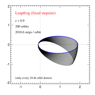
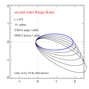
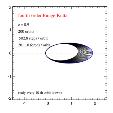
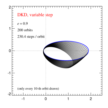
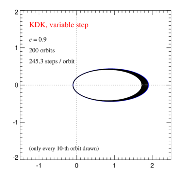
Figure 4: The upper two rows shows a Kepler problem of high eccentricity evolved with different simple time integration schemes, using an equal time step in all cases. Even though the leap-frog (upper left panel) and the second order Runge-Kutta (upper right panel) produce comparable errors in a single step, the long term stability of the integration is very different. Even a computationally much more expensive fourth order Runge-Kutta scheme (middle row), with a smaller error per step, performs dramatically worse than the leap-frog in this problem. The lower row shows the same using leap-frog schemes with a variable time step from step to step, based on the $\Delta t\propto 1/\sqrt{|{\bf{a}}|}$ criterion commonly employed in cosmological simulations. As a result of the variable time steps, the integration is no longer manifestly time reversible, and long term secular errors develop. Interestingly, the error in the KDK (Kick-Drift-Kick) variant grows four times more slowly than in the DKD (Drift-Kick-Drift) variant, despite being of equal computational cost. Taken from Springel (2005).

The accuracy obtained when evolving the system depends on the size of the time step and on the integrator scheme used. Finding the optimum size of time step is not trivial. A very simple criterion often used is

$$\Delta t=\alpha\sqrt{\epsilon/|{\bf{a}}|}$$ (23)

where $|a|$ is the acceleration obtained at the previous time step, $\epsilon$ is a length scale, which can typically be associated with the gravitational softening, and $\alpha$ is a tolerance parameter. More details about different time step criteria can be found for example in Power et al. (2003) and references therein. For the integration of the variables (positions and velocities) of the system, we only need to integrate first order equations of the form $\dot{{\bf{y}}}=f({\bf{y}})$, e.g. ordinary differential equations (ODEs) with appropriate initial conditions. Note that we can first solve this ODE for the velocity ${\bf{v}}$ and then treat $\dot{{\bf{x}}}={\bf{v}}$ as an independent ODE, at basically no extra cost.

One can distinguish implicit and explicit methods for propagating the system from step $n$ to step $n+1$. Implicit methods usually have better properties, however they need to solve the system iteratively, which usually requires inverting a matrix which is only sparsely sampled, and has the dimension of the total number of the data points, namely grid or particle points. Therefore, N-body simulations mostly adopt explicit methods.

The simplest (but never used) method to perform the integration of an ODE is called Euler’s method; here the integration is just done by multiplying the derivatives with the length of the time step. The explicit form of such a method can be written as

$${\bf{y}}_{n+1}={\bf{y}}_{n}+{\bf{f}}({\bf{y}}_{n})\Delta t,$$ (24)

whereas the implicit version is written as

$${\bf{y}}_{n+1}={\bf{y}}_{n}+{\bf{f}}({\bf{y}}_{n+1})\Delta t.$$ (25)

Note that in the latter equation ${\bf{y}}_{n+1}$ appears on the left and right side, which makes it clear why it is called implicit. Obviously the drawback of the explicit method is that it assumes that the derivatives (e.g. the forces) do not change during the time step.

An improvement to this method can be obtained by using the mean derivative during the time step, which can be written with the implicit mid-point rule as

$${\bf{y}}_{n+1}={\bf{y}}_{n}+{\bf{f}}[0.5({\bf{y}}_{n}+{\bf{y}}_{n+1})]\Delta t.$$ (26)

An explicit rule using the forces at the next time step is the so-called predictor-corrector method, where one first predicts the variables for the next time step

$${\bf{y}}_{n+1}^{0}={\bf{y}}_{n}+{\bf{f}}({\bf{y}}_{n})\Delta t$$ (27)

and then uses the forces calculated there to correct this prediction (the so-called corrector step) as

$${\bf{y}}_{n+1}={\bf{y}}_{n}+0.5[{\bf{f}}({\bf{y}}_{n})+{\bf{f}}({\bf{y}}_{n+1}^{0})]\Delta t.$$ (28)

This method is accurate to second order.

In fact, all these methods are special cases of the so-called Runge-Kutta method (RK), which achieves the accuracy of a Taylor series approach without requiring the calculation of higher order derivatives. The price one has to pay is that the derivatives (e.g. forces) have to be calculated at several points, effectively splitting the interval $\Delta t$ into special subsets. For example, a second order RK scheme can be constructed by

$${\bf{k}}_{1}={\bf{f}}({\bf{y}}_{n})$$ (29)

$${\bf{k}}_{2}={\bf{f}}({\bf{y}}_{n}+{\bf{k}}_{1}\Delta t)$$ (30)

$${\bf{y}}_{n+1}={\bf{y}}_{n}+0.5({\bf{k}}_{1}+{\bf{k}}_{2})\Delta t.$$ (31)

In a fourth order RK scheme, the time interval $\Delta t$ also has to be subsampled to calculate the mid-points, e.g.

$${\bf{k}}_{1}={\bf{f}}({\bf{y}}_{n},t_{n})$$ (32)

$${\bf{k}}_{2}={\bf{f}}({\bf{y}}_{n}+{\bf{k}}_{1}\Delta t/2,t_{n}+\Delta t/2)$$ (33)

$${\bf{k}}_{3}={\bf{f}}({\bf{y}}_{n}+{\bf{k}}_{2}\Delta t/2,t_{n}+\Delta t/2)$$ (34)

$${\bf{k}}_{4}={\bf{f}}({\bf{y}}_{n}+{\bf{k}}_{3}\Delta t/2,t_{n}+\Delta t)$$ (35)

$${\bf{y}}_{n+1}={\bf{y}}_{n}+\left(\frac{{\bf{k}}_{1}}{6}+\frac{{\bf{k}}_{2}}{3}+\frac{{\bf{k}}_{3}}{3}+\frac{{\bf{k}}_{4}}{6}\right)\Delta t.$$ (36)

More details on how to construct the coefficient for an $n$-th order RK scheme are given in e.g. Chapra & Canale (1997).

Another possibility is to use the so-called leap-frog method, where the derivatives (e.g. forces) and the positions are shifted in time by half a time step. This feature can be used to integrate directly the second order ODE of the form $\ddot{{\bf{x}}}={\bf{f}}({\bf{x}})$. Depending on whether one starts with a drift (D) of the system by half a time step or one uses the forces at the actual time to propagate the system (kick, K), one obtains a KDK version

$${\bf{v}}_{n+1/2}={\bf{v}}_{n}+{\bf{f}}({\bf{x}}_{n})\Delta t/2$$ (37)

$${\bf{x}}_{n+1}={\bf{x}}_{n}+{\bf{v}}_{n+1/2}\Delta t$$ (38)

$${\bf{v}}_{n+1}={\bf{v}}_{n+1/2}+{\bf{f}}({\bf{x}}_{n+1})\Delta t/2$$ (39)

or a DKD version of the method

$${\bf{x}}_{n+1/2}={\bf{x}}_{n}+{\bf{v}}_{n}\Delta t/2$$ (40)

$${\bf{v}}_{n+1}={\bf{v}}_{n}+{\bf{f}}({\bf{x}}_{n+1/2})\Delta t$$ (41)

$${\bf{x}}_{n+1}={\bf{x}}_{n+1/2}+{\bf{v}}_{n+1}\Delta t/2.$$ (42)

This method is accurate to second order, and, as will be shown in the next paragraph, also has other advantages. For more details see Springel (2005).

It is also clear that, depending on the application, a lower order scheme applied with more, and thus smaller, time steps can be more efficient than a higher order scheme, which enables the use of larger time steps. In the upper rows of Fig. 4, we show the numerical integration of a Kepler problem (i.e. two point-like masses with large mass difference which orbit around each other like a planet-sun system) of high eccentricity $e=0.9$, using second-order accurate leap-frog and Runga-Kutta schemes with fixed time step. There is no long-term drift in the orbital energy for the leap-frog result (left panel); only a small residual precession of the elliptical orbit is observed. On the other hand, the second-order Runge-Kutta integrator, which has formally the same error per step, fails catastrophically for an equally large time step (middle panel). After only 50 orbits, the binding energy has increased by $\sim 30$ %. If we instead employ a fourth-order Runge-Kutta scheme using the same time step (right panel), the integration is only marginally more stable, now giving a decline of the binding energy of $\sim 40$ % over 200 orbits. Note however that such a higher order integration scheme requires several force evaluations per time step, making it computationally much more expensive for a single step than the leap-frog, which requires only one force evaluation per step. The underlying mathematical reason for the remarkable stability of the leap-frog integrator lies in its symplectic properties. For a more detailed discussion, see Springel (2005).

In cosmological simulations, we are confronted with a large dynamic range in timescales. In high-density regions, like at the centres of galaxies, the required time steps are orders of magnitude smaller than in the low-density regions of the intergalactic medium, where a large fraction of the mass resides. Hence, evolving all the particles with the smallest required time step implies a substantial waste of computational resources. An integration scheme with individual time steps tries to cope with this situation more efficiently. The principal idea is to compute forces only for a certain group of particles in a given kick operation (K), with the other particles being evolved on larger time steps being usually just drifted (D) and ‘kicked’ more rarely.

The KDK scheme is hence clearly superior once one allows for individual time steps, as shown in the lower row of Fig. 4. It is also possible to try to recover the time reversibility more precisely. Hut et al. (1995) discuss an implicit time step criterion that depends both on the beginning and on the end of the time step, and, similarly, Quinn et al. (1997) discuss a binary hierarchy of trial steps that serves a similar purpose. However, these schemes are computationally impractical for large collisionless systems. Fortunately, however, in this case, the danger of building up large errors by systematic accumulation over many periodic orbits is much smaller, because the gravitational potential is highly time-dependent and the particles tend to make comparatively few orbits over a Hubble time.

2.6 Initial conditions

Figure 5: Shown is a slice to the particle distribution with the imposed displacement, taken from the same cosmological initial conditions, once based on an originally regular grid (left panel) and once based on an originally glass like particle distribution (right panel).

Having robust and well justified initial conditions is one of the key points of any numerical effort. For cosmological purposes, observations of the large–scale distribution of galaxies and of the CMB agree to good precision with the theoretical expectation that the growth of structures starts from a Gaussian random field of initial density fluctuations; this field is thus completely described by the power spectrum $P(|{\bf{k}}|)$ whose shape is theoretically well motivated and depends on the cosmological parameters and on the nature of Dark Matter.

To generate the initial conditions, one has to generate a set of complex numbers with a randomly distributed phase $\phi$ and with amplitude normally distributed with a variance given by the desired spectrum (e.g. Bardeen et al. 1986). This can be obtained by drawing two random numbers $\phi$ in $]0,1]$ and $A$ in $]0,1]$ for every point in $k$-space

$$\hat{\delta}_{{\bf{k}}}=\sqrt{-2P(|{\bf{k}}|)\mathrm{ln}(A)}{\rm e}^{i2\pi\phi}.$$ (43)

To obtain the perturbation field generated from this distribution, one needs to generate the potential $\Phi({\bf{q}})$ on a grid ${\bf{q}}$ in real space via a Fourier transform, e.g.

$$\Phi({\bf{q}})=\sum_{k}\frac{\hat{\delta}_{{\bf{k}}}}{{\bf{k}}^{2}}{\rm e}^{i{\bf{k}}{\bf{q}}}.$$ (44)

The subsequent application of the Zel’dovich approximation (Zel’dovich 1970) enables one to find the initial positions

$${\bf{x}}={\bf{q}}-D^{+}(z)\Phi({\bf{q}})$$ (45)

and velocities

$${\bf{v}}=\dot{D}^{+}(z){\bf{\nabla}}\Phi({\bf{q}})$$ (46)

of the particles, where $D^{+}(z)$ and $\dot{D}^{+}(z)$ indicate the cosmological linear growth factor and its derivative at the initial redshift $z$. A more detailed description can be found in e.g. Efstathiou et al. (1985).

There are two further complications which should be mentioned. The first is that one can try to reduce the discreteness effect that is induced on the density power spectrum by the regularity of the underlying grid of the particle positions ${\bf{q}}$ that one has at the start. This can be done by constructing an amorphous, fully relaxed particle distribution to be used, instead of a regular grid. Such a particle distribution can be constructed by applying negative gravity to a system and evolving it for a long time, including a damping of the velocities, until it reaches a relaxed state, as suggested by White (1996). Fig. (5) gives a visual impression on the resulting particle distributions.

A second complication is that, even for studying individual objects like galaxy clusters, large-scale tidal forces can be important. A common approach used to deal with this problem is the so-called “zoom” technique: a high resolution region is self-consistently embedded in a larger scale cosmological volume at low resolution (see e.g. Tormen et al. 1997). This approach usually allows an increase of the dynamical range of one to two orders of magnitude while keeping the full cosmological context. For galaxy simulations it is even possible to apply this technique on several levels of refinements to further improve the dynamical range of the simulation (e.g. Stoehr et al. 2003). A frequently used, publicly available package to create initial conditions is the COSMICS package by Bertschinger (1995).

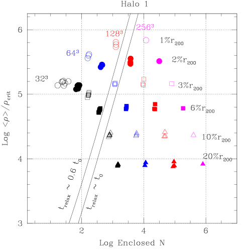
Figure 6: Mean inner density contrast as a function of the enclosed number of particles in 4 series of simulations varying the number of particles in the high-resolution box, from $32^{3}$ to $256^{3}$. Each symbol corresponds to a fixed fraction of the virial radius, as shown by the labels on the right. The number of particles needed to obtain robust results increases with density contrast, roughly as prescribed by the requirement that the collisional relaxation timescale should remain longer than the age of the Universe. According to this, robust numerical estimates of the mass profile of a halo are only possible to the right of the curve labelled $t_{\rm relax}\sim 0.6t_{0}$. Taken from Power et al. (2003).

2.7 Resolution

There has been a long standing discussion in the literature to understand what is the optimal setup for cosmological simulations, and how many particles are needed to resolve certain regions of interest. Note that the number of particles needed for convergence also depends on what quantity one is interested in. For example, mass functions, which count identified haloes, usually give converging results at very small particle numbers per halo ($\approx 30-50$), whereas structural properties, like a central density or the virial radius, converge only at significantly higher particle numbers ($\approx 1000$). As we will see in a later chapter, if one wants to infer hydrodynamical properties like baryon fraction or X-ray luminosity, values converge only for haloes represented by even more particles ($\approx 10\,000$).

Recently, Power et al. (2003) performed a comprehensive series of convergence tests designed to study the effect of numerical parameters on the structure of simulated CDM haloes. These tests explore the influence of the gravitational softening, the time stepping algorithm, the starting redshift, the accuracy of force computations, and the number of particles in the spherically-averaged mass profile of a galaxy-sized halo in the CDM cosmogony with a non-null cosmological constant ($\Lambda$CDM). Power et al. (2003), and the references therein, suggest empirical rules that optimise the choice of these parameters. When these choices are dictated by computational limitations, Power et al. (2003) offer simple prescriptions to assess the effective convergence of the mass profile of a simulated halo. One of their main results is summarised in Fig. 6, which shows the convergence of a series of simulations with different mass resolution on different parts of the density profile of a collapsed object. This figure clearly demonstrates that the number of particles within a certain radius needed to obtain converging results depends on the enclosed density.

In general, both the size and the dynamical range or resolution of the simulations have been increasing very rapidly over the last decades. Fig. 7 shows a historical compilation of large N-body simulations: their size growth, thanks to improvements in the algorithms, is faster than the underlying growth of the available CPU power.

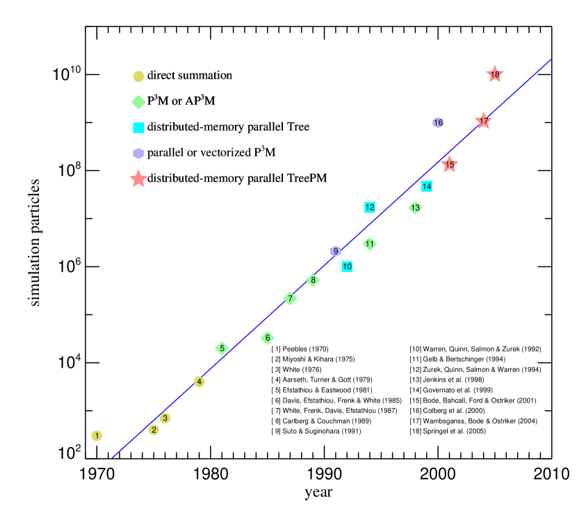
Figure 7: Moore’s empirical law shows that the computing power typically doubles every 18 months. This figure shows the size of N-body simulations as a function of their running date. Clearly, specially recently, the improvement in the algorithms allowed the simulation to grow faster than the improvement of the underlying CPU power. Kindly provided by Volker Springel.

2.8 Code comparison for pure gravity

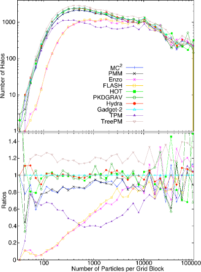
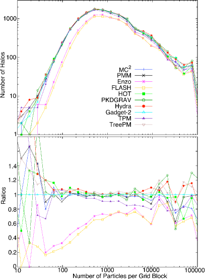
Figure 8: A recent comparison of the predicted number of halos as a function of density for ten different cosmological codes. Left panel: halos with $10-40$ particles, right panel: halos with $41-2500$ particles. The lower panels show the residuals with respect to GADGET-2. Both panels show the deficit of small halos in ENZO and FLASH over most of the density region – only at very high densities do the results catch up. The behaviour of the TPM simulation is interesting: not only does this simulation have a deficit of small halos but the deficit is very significant in medium density regions, in fact falling below the two Adaptive Mesh Refinement codes. The slight excess of small halos shown in the TreePM run vanishes completely if the halo cut is raised to 20 particles per halo and the TreePM results are in that case in excellent agreement with GADGET-2. Adapted from Heitmann et al. (2007).

In the last thirty years cosmology has turned from a science of order-of-magnitude estimates to a science with accuracies of 10 % or less in its measurements and theoretical predictions. Crucial observations along the way were the measurement of the cosmic microwave background radiation, and large galaxy surveys. In the future such observations will yield even higher accuracy (1 %) over a much wider dynamical range. Such measurements will provide insight into several topics, e.g. the nature of dark energy (expressed by the equation of state $w=p/\rho$ with $p$ being the pressure and $\rho$ the density). In order to make optimal use of the observations, theoretical calculations of at least the same level of accuracy are required. As physics in the highly non-linear regime, combined with complicated gas physics and astrophysical feedback processes are involved, this represents a real challenge.

Different numerical methods have therefore to be checked and compared continuously. The most recent comparison of ten commonly-used codes from the literature has been performed in an extensive comparison program. The ten codes used for the comparison performed by Heitmann et al. (2007) cover a variety of methods and application arenas. The simulation methods employed include parallel particle-in-cell (PIC) techniques (the PM codes MC² and PMM, the Particle-Mesh / Adaptive Mesh Refinement (AMR) codes ENZO and FLASH), a hybrid of PIC and direct N-body (the AP³M code Hydra), tree algorithms (the treecodes PKDGRAV and HOT), and hybrid tree-PM algorithms (GADGET-2, TPM, and TreePM).

The results from the code comparisons are satisfactory and not unexpected, but also show that much more work is needed in order to attain the required accuracy for upcoming surveys. The halo mass function is a very stable statistic, the agreement over wide ranges of mass being better than 5 %. Additionally, the low mass cutoff for individual codes can be reliably predicted by a simple criterion.

The internal structure of halos in the outer regions of $\sim R_{200}$ also appears to be very similar between different simulation codes. Larger differences between the codes in the inner region of the halos occur if the halo is not in a relaxed state: in this case, time stepping issues might also play an important role (e.g. particle orbit phase errors, global time mismatches). For halos with a clear single centre, the agreement is very good and predictions for the fall-off of the profiles from resolution criteria hold as expected. The investigation of the halo counts as a function of density revealed an interesting problem with the TPM code, the simulation suffering from a large deficit in medium density regimes. The AMR codes showed a large deficit of small halos over almost the entire density regime, as the base grid of the AMR simulation sets a resolution limit that is too low for the halos, as can be seen in Figure (8).

The power spectrum measurements revealed definitively more scatter among the different codes than expected. The agreement in the nonlinear regime is at the $5-10$ % level, even on moderate spatial scales around $k=10h$ Mpc^-1. This disagreement on small scales is connected to differences of the codes in the inner regions of the halos. For more detailed discussion see Heitmann et al. (2007) and references therein.

In a detailed comparison of ENZO and GADGET, O’Shea et al. (2005) already pointed out that to reach reasonable good agreement, relatively conservative criteria for the adaptive grid refinement are needed. Furthermore, choosing a grid resolution twice as high as the mean inter-particle distance of the dark matter particles is recommended, to improve the small scale accuracy of the calculation of the gravitational forces.

3 Hydro methods

The baryonic content of the Universe can typically be described as an ideal fluid. Therefore, to follow the evolution of the fluid, one usually has to solve the set of hydrodynamic equations

$$\frac{\mathrm{d}{\bf{v}}}{\mathrm{d}t}=-\frac{{\bf{\nabla}}P}{\rho}-{\bf{\nabla}}\Phi,$$ (47)

$$\frac{\mathrm{d}\rho}{\mathrm{d}t}+\rho{\bf{\nabla}}{\bf{v}}=0$$ (48)

and

$$\frac{\mathrm{d}u}{\mathrm{d}t}=-\frac{P}{\rho}{\bf{\nabla}}\cdot{\bf{v}}-\frac{\Lambda(u,\rho)}{\rho},$$ (49)

which are the Euler equation, continuity equation and the first law of thermodynamics, respectively. They are closed by an equation of state, relating the pressure $P$ to the internal energy (per unit mass) $u$. Assuming an ideal, monatomic gas, this will be

$$P=(\gamma-1)\rho u$$ (50)

with $\gamma=5/3$. In the next sections, we will discuss how to solve this set of equations, neglecting radiative losses described by the cooling function $\Lambda(u,\rho)$; in Sect. 4.1 we will give examples of how radiative losses or additional sources of heat are included in cosmological codes. We can also assume that the ${\bf{\nabla}}\Phi$ term will be solved using the methods described in the previous section.

As a result of the high nonlinearity of gravitational clustering in the Universe, there are two significant features emerging in cosmological hydrodynamic flows; these features pose more challenges than the typical hydrodynamic simulation without self-gravity. One significant feature is the extremely supersonic motion around the density peaks developed by gravitational instability, which leads to strong shock discontinuities within complex smooth structures. Another feature is the appearance of an enormous dynamic range in space and time, as well as in the related gas quantities. For instance, the hierarchical structures in the galaxy distribution span a wide range of length scales, from the few kiloparsecs resolved in an individual galaxy to the several tens of megaparsecs characterising the largest coherent scale in the Universe.

A variety of numerical schemes for solving the coupled system of collisional baryonic matter and collisionless dark matter have been developed in the past decades. They fall into two categories: particle methods, which discretise mass, and grid-based methods, which discretise space. We will briefly describe both methods in the next two sections.

3.1 Eulerian (grid)

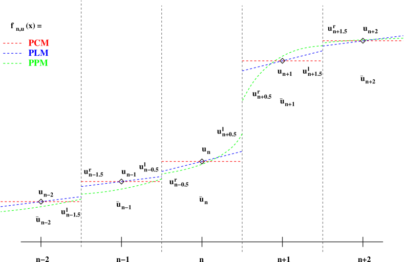
Figure 9: Reconstruction of the principal variables ($u_{n}$) on the grid using different methods, like piecewise constant (PCM), piecewise linear (PLM) or piecewise parabolic (PPM). The reconstruction scheme then allows one to calculate cell averages ($\bar{u}_{n}$) as well as the left and right-hand sided values on the cell boundaries ($u_{n\pm 0.5}^{l}$,$u_{n\pm 0.5}^{r}$).

The set of hydrodynamical equations for an expanding Universe reads

$$\frac{\partial{\bf{v}}}{\partial t}+\frac{1}{a}({\bf{v}}\cdot{\bf{\nabla}}){\bf{v}}+\frac{\dot{a}}{a}{\bf{v}}=-\frac{1}{a\rho}{\bf{\nabla}}P-\frac{1}{a}{\bf{\nabla}}\Phi,$$ (51)

$$\frac{\partial\rho}{\partial t}+\frac{3\dot{a}}{a}\rho+\frac{1}{a}{\bf{\nabla}}\cdot(\rho{\bf{v}})=0$$ (52)

and

$$\frac{\partial}{\partial t}(\rho u)+\frac{1}{a}{\bf{v}}\cdot{\bf{\nabla}}(\rho u)=-(\rho u+P)\left(\frac{1}{a}{\bf{\nabla}}\cdot{\bf{v}}+3\frac{\dot{a}}{a}\right)$$ (53)

respectively, where the right term in the last equation reflects the expansion in addition to the usual $P\mathrm{d}V$ work.

The grid-based methods solve these equations based on structured or unstructured grids, representing the fluid. One distinguishes primitive variables, which determine the thermodynamic properties, (e.g $\rho$, ${\bf{v}}$ or $P$) and conservative variables which define the conservation laws, (e.g. $\rho$, $\rho{\bf{v}}$ or $\rho u$). Early attempts were made using a central difference scheme, where fluid is only represented by the centred cell values (e.g. central variables, $u_{n}$ in Fig. 9 and derivatives are obtained by the finite-difference representation, similar to Eq. 15 and 16, see for example Cen (1992). Such methods will however break down in regimes where discontinuities appear. These methods therefore use artificial viscosity to handle shocks (similar to the smoothed particle hydrodynamics method described in the next section). Also, by construction, they are only first-order accurate.

More modern approaches use reconstruction schemes, which, depending on their order, take several neighbouring cells into account to reconstruct the field of any hydrodynamical variable. Fig. 9 illustrates three different reconstruction schemes, with increasing order of accuracy, as piecewise constant method (PCM), piecewise linear method (PLM, e.g. Colella & Glaz 1985) and piecewise parabolic method (PPM, Colella & Woodward 1984). The shape of the reconstruction $f_{n,u}(x)$ is then used to calculate the total integral of a quantity over the grid cell, divided by the volume of each cell (e.g. cell average, $\hat{u}_{n}$), rather than pointwise approximations at the grid centres (e.g. central variables, $u_{n}$).

$$\hat{u}_{n}=\int\limits_{x_{n-0.5}}^{x_{n+0.5}}f_{n,u}(x)\mathrm{d}x$$ (54)

They are also used to calculate the left and right-hand sided values at the cell boundaries (e.g. $u_{n\pm 0.5}^{l}$,$u_{n\pm 0.5}^{r}$), which are used later as initial conditions to solve the Riemann problem. To avoid oscillations (e.g. the development of new extrema), additional constraints are included in the reconstruction. For example, in the PLM reconstruction this is ensured by using so-called slope limiters which estimate the maximum slope allowed for the reconstruction. One way is to demand that the total variation among the interfaces does not increase with time. Such so-called total variation diminishing schemes (TVD, Harten 1983), nowadays provide various different slope limiters suggested by different authors. In our example illustrated by Fig. 9, the so called minmod slope limiter

$$\overline{\Delta u_{i}}=\mathrm{minmod}\left(\Theta(u_{i+1}-u_{i}),(u_{i+1}-u_{i-1})/2,\theta(u_{i}-u_{i-1})\right),$$ (55)

where $\overline{\Delta u_{i}}$ is the limiter slope within the cell $i$ and $\theta=[1,2]$, would try to fix the slope $f^{\prime}_{n-1,u}(x_{n-1})$ and $f^{\prime}_{n,u}(x_{n})$, such as to avoid that $u_{n-0.5}^{l}$ becomes larger than $u_{n-0.5}^{r}$. The so called Aldaba-type limiter

$$\overline{\Delta u_{i}}=\frac{2(u_{i+1}-u_{i})(u_{i}-u_{i-1})+\epsilon}{(u_{i+1}-u_{i})^{2}+(u_{i}-u_{i-1})^{2}+\epsilon^{2}}\frac{1}{2}(u_{i+1}-u_{i-1}),$$ (56)

where $\epsilon$ is a small positive number to avoid problems in homogeneous regions, would try to avoid that $u_{n-0.5}^{l}$ is getting larger than $u_{n}$ and that $u_{n-0.5}^{r}$ is getting smaller than $u_{n-1}$, e.g. that a monotonic profile in $u_{i}$ is preserved.

In the PPM (or even higher order) reconstruction this enters as an additional condition when finding the best-fitting polynomial function. The additional cells which are involved in the reconstruction are often called the stencil. Modern, high order schemes usually have stencils based on at least 5 grid points and implement essentially non-oscillatory (ENO; Harten et al. 1987) or monoticity preserving (MP) methods for reconstruction, which maintain high-order accuracy. For every reconstruction, a smoothness indicator $S_{n}^{m}$ can be constructed, which is defined as the integral over the sum of the squared derivatives of the reconstruction over the stencil chosen, e.g.

$$S_{n}^{m}=\sum_{l=1}^{2}\int\limits_{x_{n-m}}^{x_{n+m}}(\Delta x)^{2l-1}\left(\partial_{x}^{l}f_{n,u}^{m}(x)\right)^{2}\mathrm{d}V.$$ (57)

In the ENO schemes, a set of candidate polynomials $p_{n}^{m}$ with order $2m+1$ for a set of stencils based on different numbers of grid cells $m$ are used to define several different reconstruction functions $f_{n,u}^{m}$. Then, the reconstruction with the lowest smoothness indicator $S_{n}^{m}$ is chosen. In this way the order of reconstruction will be reduced around discontinuities, and oscillating behaviour will be suppressed.

To improve on the ENO schemes in robustness and accuracy one can, instead of selecting the reconstruction with the best smoothness indicator $S_{n}^{m}$, construct the final reconstruction by building the weighted reconstruction

$$\hat{f}_{u}(x)=\sum_{m}w_{m}f_{n,u}^{m}(x),$$ (58)

where the weights $w_{m}$ are a proper function of the smoothness indicators $S_{n}^{m}$. This procedure is not unique. Jiang & Shu (1996) proposed defining

$$w_{m}=\frac{\alpha_{m}}{\sum_{l}\alpha_{l}}$$ (59)

with

$$\alpha_{l}=\frac{C_{l}}{(\epsilon+S_{n}^{l})^{\beta}},$$ (60)

where $C_{l}$, $\epsilon$ and $\beta$ are free parameters, which for example can be taken from Levy et al. (1999). This are the so-called weighted essentially non-oscillatory (WENO) schemes. These schemes can simultaneously provide a high-order resolution for the smooth part of the solution and a sharp, monotonic shock or contact discontinuity transition. For a review on ENO and WENO schemes, see e.g. Shu (1998).

After the left and right-hand values at the cell boundaries (e.g. interfaces) are reconstructed, the resulting Riemann problem is solved, e.g. the evolution of two constant states separated by a discontinuity. This can be done either analytically or approximately, using left and right-handed values at the interfaces as a jump condition.

With the solution one obtains, the fluxes across these boundaries for the time step can be calculated and the cell averages $\hat{u}_{n}$ can be updated accordingly. In multiple dimensions, all these steps are performed for each coordinate direction separately, taking only the interface values along the individual axes into account. There are attempts to extend the reconstruction schemes, to directly reconstruct the principal axis of the Riemann problem in multiple dimensions, so that then it has to be solved only once for each cell. However the complexity of reconstructing the surface of shocks in three dimensions has so far seen to be untraceable.

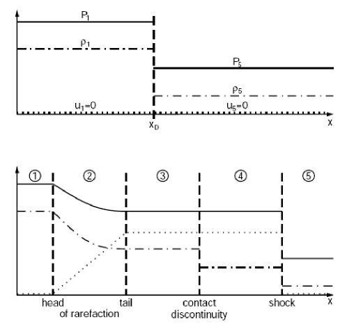
Figure 10: The Riemann problem: The upper panel shows the initial state, the lower panel shows the evolved problem for the case of no relative motion between the two sides ($u_{1}=u_{5}=0$). The solid lines mark the pressure $P$, the dashed dotted lines the density $\rho$ and the dotted line the velocity $v$. Kindly provided by Ewald Müller.

How to solve the general Riemann problem, e.g. the evolution of a discontinuity initially separating two states, can be found in text books (e.g. Courant & Friedrichs 1948). Here we give only the evolution of a shock tube as an example. This corresponds to a system where both sides are initially at rest. Fig. 10 shows the initial and the evolved system. The latter can be divided into 5 regions. The values for regions 1 and 5 are identical to the initial configuration. Region 2 is a rarefaction wave which is determined by the states in region 1 and 3. Therefore we are left with 6 variables to determine, namely $\rho_{3}$, $P_{3}$, $v_{3}$ and $\rho_{4}$, $P_{4}$, $v_{4}$, where we have already eliminated the internal energy $u_{i}$ in all regions, as it can be calculated from the equation of state. As there is no mass flux through the contact discontinuity, and as the pressure is continuous across the contact discontinuity, we can eliminate two of the six variables by setting $v_{3}=v_{4}=v_{\rm c}$ and $P_{3}=P_{4}=P_{\rm c}$. The general Rankine-Hugoniot conditions, describing the jump conditions at a discontinuity, read

$$\rho_{l}v_{l} = \rho_{r}v_{r}$$ (61)

$$\rho_{l}v_{l}^{2}+P_{l} = \rho_{r}v_{r}^{2}+P_{r}$$ (62)

$$v_{l}\left(\rho_{l}(v_{l}^{2}/2+u_{l})+P_{l}\right) = v_{r}\left(\rho_{r}(v_{r}^{2}/2+u_{r})+P_{r}\right),$$ (63)

where we have assumed a coordinate system which moves with the shock velocity $v_{\rm s}$. Assuming that the system is at rest in the beginning, e.g. $v_{1}=v_{5}=0$, the first Rankine-Hugoniot condition for the shock between region 4 and 5 moving with a velocity $v_{\rm s}$ (note the implied change of the coordinate system) is in our case

$$m=\rho_{5}v_{\rm s}=\rho_{4}(v_{\rm s}-v_{\rm c})$$ (64)

and therefore the shock velocity becomes

$$v_{\rm s}=\frac{\rho_{4}v_{\rm c}}{\rho_{4}-\rho_{5}}.$$ (65)

The second Rankine-Hugoniot condition is

$$mv_{\rm c}=\rho_{4}(v_{\rm s}-v_{\rm c})v_{\rm c}=P_{\rm c}-P_{5},$$ (66)

which, combined with the first, can be written as

$$\rho_{4}\left(\frac{\rho_{4}v_{\rm c}}{\rho_{4}-\rho_{5}}-v_{\rm c}\right)v_{\rm c}=P_{\rm c}-P_{5},$$ (67)

which, slightly simplified, leads to a first condition

$$(P_{5}-P_{\rm c})\left(\frac{1}{\rho_{5}}-\frac{1}{\rho_{4}}\right)=-v_{\rm c}^{2}.$$ (68)

The third Rankine-Hugoniot condition is

$$m(\epsilon_{4}+\frac{v_{\rm c}^{2}}{2}-\epsilon_{5})=P_{\rm c}v_{\rm c},$$ (69)

which, by eliminating $m$, can be written as

$$\epsilon_{4}-\epsilon_{5}=\frac{P_{\rm c}+P_{5}}{P_{\rm c}-P_{5}}\frac{v_{\rm c}^{2}}{2}.$$ (70)

Using the first condition (Eq. 68) and assuming an ideal gas for the equation of state, one gets

$$\frac{1}{\gamma-1}\left(\frac{P_{\rm c}}{\rho_{4}}-\frac{P_{5}}{\rho_{5}}\right)=\frac{P_{\rm c}+P_{5}}{2\rho_{4}\rho_{5}},$$ (71)

which leads to the second condition

$$\frac{P_{\rm c}-P_{5}}{P_{\rm c}+P_{5}}=\gamma\frac{\rho_{4}-\rho_{5}}{\rho_{4}+\rho_{5}}.$$ (72)

The third condition comes from the fact that the entropy ($\propto\ln(P/\rho^{\gamma})$ stays constant in the rarefaction wave, and therefore one can write it as

$$\frac{P_{1}}{P_{\rm c}}=\left(\frac{\rho_{1}}{\rho_{3}}\right)^{\gamma}.$$ (73)

The fourth condition comes from the fact that the Riemann Invariant

$$v+\int\frac{c}{\rho}\mathrm{d}\rho$$ (74)

is a constant, which means that

$$v_{\rm c}+\int\frac{c_{3}}{\rho_{3}}\mathrm{d}\rho=v_{1}+\int\frac{c_{1}}{\rho_{1}}\mathrm{d}\rho,$$ (75)

where $c=\sqrt{\gamma P/\rho}$ denotes the sound velocity, with which the integral can be written as

$$\int\frac{c}{\rho}\mathrm{d}\rho=\frac{2}{\gamma-1}\sqrt{\frac{\gamma P}{\rho}}.$$ (76)

Therefore, the fourth condition can be written as

$$v_{\rm c}+\frac{2}{\gamma-1}\sqrt{\frac{\gamma P_{\rm c}}{\rho_{3}}}=\frac{2}{\gamma-1}\sqrt{\frac{\gamma P_{1}}{\rho_{1}}}.$$ (77)

Combining all 4 conditions (equations 68, 72, 73 and 77) and defining the initial density ratio $\lambda=\rho_{1}/\rho_{5}$ one gets the non linear, algebraic equation

$$\frac{\rho_{1}}{\rho_{5}}\frac{1}{\lambda}\frac{(1-P)^{2}}{\gamma(1+P)-1+P}=\frac{2\gamma}{(\gamma-1)^{2}}\left[1-\left(\frac{P}{\lambda}\right)^{(\gamma-1)/(2\gamma)}\right]^{2}$$ (78)

for the pressure ratio $P=P_{\rm c}/P_{5}$. Once $P_{\rm c}$ is known from solving this equation, the remaining unknowns can be inferred step by step from the four conditions.

There are various approximate methods to solve the Riemann problem, including the so-called ROE method (e.g. Powell et al. 1999), HLL/HLLE method (e.g. see Harten et al. 1983; Einfeldt 1988; Einfeldt et al. 1991) and HLLC (e.g. see Li 2005). A description of all these methods is outside the scope of this review, so we redirect the reader to the references given or textbooks like LeVeque (2002).

At the end of each time step, one has to compute the updated central values $u_{n}$ from the updated cell average values $\hat{u}_{n}$. Normally, this would imply inverting equation (54), which is not trivial in the general case. Therefore, usually an additional constraint is placed on the reconstruction method, namely that the reconstruction fulfills $u_{n}=\hat{u}_{n}$. In this case the last step is trivial.

In general, the grid-based methods suffer from limited spatial resolution, but they work extremely well in both low- and high-density regions, as well as in shocks. In cosmological simulations, accretion flows with large Mach numbers (e.g. $M>100$) are very common. Here, following the total energy in the hydrodynamical equations, one can get inaccurate thermal energy, leading to negative pressure, due to discretisation errors when the kinetic energy dominates the total energy. In such cases, as suggested by Ryu et al. (1993) and Bryan et al. (1995), the numerical schemes usually switch from formulations solving the total energy to formulations based on solving the internal energy in these hypersonic flow regions.

In the cosmological setting, there are the TVD-based codes including those of Ryu et al. (1993) and Li et al. (2006) (CosmoMHD), the moving-mesh scheme (Pen 1998) and the PLM-based code ART (Kravtsov et al. 1997; Kravtsov 2002). The PPM-based codes include those of Stone & Norman (1992) (Zeus), Bryan et al. (1995) (ENZO), Ricker et al. (2000) (COSMOS) and Fryxell et al. (2000) (FLASH). There is also the WENO-based code by Feng et al. (2004).

3.2 Langrangian (SPH)

The particle methods include variants of smoothed particle hydrodynamics (SPH; Gingold & Monaghan 1977; Lucy 1977) such as those of Evrard (1988), Hernquist & Katz (1989), Navarro & White (1993), Couchman et al. (1995) (Hydra), Steinmetz (1996a) (GRAPESPH), Owen et al. (1998), and Springel et al. (2001a); Springel (2005) (GADGET). The SPH method solves the Lagrangian form of the Euler equations and can achieve good spatial resolutions in high-density regions, but it works poorly in low-density regions. It also suffers from degraded resolution in shocked regions due to the introduction of a sizable artificial viscosity. Agertz et al. (2007) argued that whilst Eulerian grid-based methods are able to resolve and treat dynamical instabilities, such as Kelvin-Helmholtz or Rayleigh-Taylor, these processes are poorly resolved by existing SPH techniques. The reason for this is that SPH, at least in its standard implementation, introduces spurious pressure forces on particles in regions where there are steep density gradients, in particular near contact discontinuities. This results in a boundary gap of the size of an SPH smoothing kernel radius, over which interactions are severely damped. Nevertheless, in the cosmological context, the adaptive nature of the SPH method compensates for such shortcomings, thus making SPH the most commonly used method in numerical hydrodynamical cosmology.

3.2.1 Basics of SPH

The basic idea of SPH is to discretise the fluid by mass elements (e.g. particles), rather than by volume elements as in the Eulerian methods. Therefore it is immediately clear that the mean inter-particle distance in collapsed objects will be smaller than in underdense regions; the scheme will thus be adaptive in spatial resolution by keeping the mass resolution fixed. For a comprehensive review see Monaghan (1992). To build continuous fluid quantities, one starts with a general definition of a kernel smoothing method

$$\left<A({\bf{x}})\right>=\int W({\bf{x}}-{\bf{x}}^{\prime},h)A({\bf{x}}^{\prime})\mathrm{d}{\bf{x}}^{\prime},$$ (79)

which requires that the kernel is normalised (i.e. $\int W({\bf{x}},h)\mathrm{d}{\bf{x}}=1$) and collapses to a delta function if the smoothing length $h$ approaches zero, namely $W({\bf{x}},h)\rightarrow\delta({\bf{x}})$ for $h\rightarrow 0$.

One can write down the continuous fluid quantities (e.g. $\left<A({\bf{x}})\right>$) based on the discretised values $A_{j}$ represented by the set of the individual particles $m_{j}$ at the position ${\bf{x}}_{j}$ as

$$\left<A_{i}\right>=\left<A({\bf{x}}_{i})\right>=\sum_{j}\frac{m_{j}}{\rho_{j}}A_{j}W({\bf{x}_{i}}-{\bf{x}_{j}},h)\,,$$ (80)

where we assume that the kernel depends only on the distance modulus (i.e. $W(|{\bf{x}}-{\bf{x}}^{\prime}|,h)$) and we replace the volume element of the integration, $\mathrm{d}{\bf{x}}=\mathrm{d}^{3}x$, with the ratio of the mass and density $m_{j}/\rho_{j}$ of the particles. Although this equation holds for any position ${\bf{x}}$ in space, here we are only interested in the fluid representation at the original particle positions ${\bf{x}}_{i}$, which are the only locations where we will need the fluid representation later on. It is important to note that for kernels with compact support (i.e. $W({\bf{x}},h)=0$ for $|{\bf{x}}|>h$) the summation does not have to be done over all the particles, but only over the particles within the sphere of radius $h$, namely the neighbours around the particle $i$ under consideration. Traditionally, the most frequently used kernel is the $B_{2}$-spline, which can be written as

$$W(x,h)=\frac{\sigma}{h^{\nu}}\left\{\begin{array}[]{ll}1-6\left(\frac{x}{h}\right)^{2}+6\left(\frac{x}{h}\right)^{3}&0\leq\frac{x}{h}<0.5\\ 2\left(1-\frac{x}{h}\right)^{3}&0.5\leq\frac{x}{h}<1\\ 0&1\leq\frac{x}{h}\\ \end{array}\right.,$$ (81)

where $\nu$ is the dimensionality (e.g. 1, 2 or 3) and $\sigma$ is the normalisation

$$\sigma=\left\{\begin{array}[]{ll}\frac{16}{3}&\nu=1\\ \frac{80}{7\pi}&\nu=2\\ \frac{8}{\pi}&\nu=3\;.\\ \end{array}\right.$$ (82)

Sometimes, spline kernels of higher order are used for very special applications; however the $B_{2}$ spline kernel turns out to be the optimal choice in most cases.

When one identifies $A_{i}$ with the density $\rho_{i}$, $\rho_{i}$ cancels out on the right hand side of Eq. 80, and we are left with the density estimate

$$\left<\rho_{i}\right>=\sum_{j}m_{j}W({\bf{x}_{i}}-{\bf{x}_{j}},h),$$ (83)

which we can interpret as the density of the fluid element represented by the particle $i$.

Now even derivatives can be calculated as

$${\bf{\nabla}}\left<A_{i}\right>=\sum_{j}\frac{m_{j}}{\rho_{j}}A_{j}{\bf{\nabla}}_{i}W({\bf{x}_{i}}-{\bf{x}_{j}},h),$$ (84)

where ${\bf{\nabla}}_{i}$ denotes the derivative with respect to ${\bf{x}}_{i}$. A pairwise symmetric formulation of derivatives in SPH can be obtained by making use of the identity

$$(\rho{\bf{\nabla}})\cdot{}A={\bf{\nabla}}(\rho\cdot{}A)-\rho\cdot({\bf{\nabla}}A),$$ (85)

which allows one to re-write a derivative as

$${\bf{\nabla}}\left<A_{i}\right>=\frac{1}{\rho_{i}}\sum_{j}m_{j}(A_{j}-A_{i}){\bf{\nabla}}_{i}W({\bf{x}_{i}}-{\bf{x}_{j}},h).$$ (86)

Another way of symmetrising the derivative is to use the identity

$$\frac{{\bf{\nabla}}A}{\rho}={\bf{\nabla}}\left(\frac{A}{\rho}\right)+\frac{A}{\rho^{2}}{\bf{\nabla}}\rho,$$ (87)

which then leads to the following form of the derivative:

$${\bf{\nabla}}\left<A_{i}\right>=\rho_{i}\sum_{j}m_{j}\left(\frac{A_{j}}{\rho_{j}^{2}}+\frac{A_{i}}{\rho_{i}^{2}}\right){\bf{\nabla}}_{i}W({\bf{x}_{i}}-{\bf{x}_{j}},h).$$ (88)

3.2.2 The fluid equations

By making use of these identities, the Euler equation can be written as

$$\frac{\mathrm{d}{\bf{v}}_{i}}{\mathrm{d}t}=-\sum_{j}m_{j}\left(\frac{P_{j}}{\rho_{j}^{2}}+\frac{P_{i}}{\rho_{i}^{2}}+\Pi_{ij}\right){\bf{\nabla}}_{i}W({\bf{x}_{i}}-{\bf{x}_{j}},h).$$ (89)

By combining the above identities and averaging the result, the term $-(P/\rho){\bf{\nabla}}\cdot{\bf{v}}$ from the first law of thermodynamics can similarly be written as

$$\frac{\mathrm{d}u_{i}}{\mathrm{d}t}=\frac{1}{2}\sum_{j}m_{j}\left(\frac{P_{j}}{\rho_{j}^{2}}+\frac{P_{i}}{\rho_{i}^{2}}+\Pi_{ij}\right)\left({\bf{v}}_{j}-{\bf{v}}_{i}\right){\bf{\nabla}}_{i}W({\bf{x}_{i}}-{\bf{x}_{j}},h).$$ (90)

Here we have added a term $\Pi_{ij}$ which is the so-called artificial viscosity. This term is usually needed to capture shocks and its construction is similar to other hydro-dynamical schemes. Usually, one adopts the form proposed by Monaghan & Gingold (1983) and Balsara (1995), which includes a bulk viscosity and a von Neumann-Richtmeyer viscosity term, supplemented by a term controlling angular momentum transport in the presence of shear flows at low particle numbers (Steinmetz 1996b). Modern schemes implement a form of the artificial viscosity as proposed by Monaghan (1997) based on an analogy with Riemann solutions of compressible gas dynamics. To reduce this artificial viscosity, at least in those parts of the flows where there are no shocks, one can follow the idea proposed by Morris & Monaghan (1997): every particle carries its own artificial viscosity, which eventually decays outside the regions which undergo shocks. A detailed study of the implications on the ICM of such an implementation can be found in Dolag et al. (2005).

The continuity equation does not have to be evolved explicitly, as it is automatically fulfilled in Lagrangian methods. As shown earlier, density is no longer a variable but can be, at any point, calculated from the particle positions. Obviously, mass conservation is guaranteed, unlike volume conservation: in other words, the sum of the volume elements associated with all of the particles might vary with time, especially when strong density gradients are present.

3.2.3 Variable smoothing length

Usually, the smoothing length $h$ will be allowed to vary for each individual particle $i$ and is determined by finding the radius $h_{i}$ of a sphere which contains $n$ neighbours. Typically, different numbers $n$ of neighbours are chosen by different authors, ranging from 32 to 80. In principle, depending on the kernel, there is an optimal choice of neighbours (e.g. see Silverman 1986 or similar books). However, one has to find a compromise between a large number of neighbours, leading to larger systematics but lower noise in the density estimates (especially in regions with large density gradients) and a small number of neighbours, leading to larger sample variances for the density estimation. In general, once every particle has its own smoothing length, a symmetric kernel $W({\bf{x}}_{i}-{\bf{x}}_{j},h_{i},h_{j})={\bar{W}}_{ij}$ has to be constructed to keep the conservative form of the formulations of the hydrodynamical equations. There are two main variants used in the literature: one is the kernel average ${\bar{W}}_{ij}=(W({\bf{x}}_{i}-{\bf{x}}_{j},h_{i})+W({\bf{x}}_{i}-{\bf{x}}_{j},h_{j}))/2$, the other is an average of the smoothing length ${\bar{W}}_{ij}=W({\bf{x}}_{i}-{\bf{x}}_{j},(h_{i}+h_{j})/2)$. The former is the most commonly used approach.

Note that in all of the derivatives discussed above, it is assumed that $h$ does not depend on the position ${\bf{x}}_{j}$. Thus, by allowing the smoothing length $h_{i}$ to be variable for each particle, one formally neglects the correction term $\partial W/\partial h$, which would appear in all the derivatives. In general, this correction term cannot be computed trivially and therefore many implementations do not take it into account. It is well known that such formulations are poor at conserving numerically both internal energy and entropy at the same time, independently of the use of internal energy or entropy in the formulation of the first law of thermodynamics, see Hernquist (1993). In the next subsection, we present a way of deriving the equations which include these correction terms $\partial W/\partial h$; this equation set represents a formulation which conserves numerically both entropy and internal energy.

3.2.4 The entropy conservation formalism

To derive a better formulation of the SPH method, Springel & Hernquist (2002) started from the entropic function $A=P/\rho^{\gamma}$, which will be conserved in adiabatic flows. The internal energy per unit mass can be inferred from this entropic function as

$$u_{i}=\frac{A_{i}}{\gamma-1}\rho_{i}^{\gamma-1}$$ (91)

at any time, if needed. Entropy will be generated by shocks, which are captured by the artificial viscosity $\Pi_{ij}$ and therefore the entropic function will evolve as

$$\frac{\mathrm{d}A_{i}}{\mathrm{d}t}=\frac{1}{2}\frac{\gamma-1}{\rho_{i}^{\gamma-1}}\sum_{j}m_{j}\Pi_{ij}\left({\bf{v}}_{j}-{\bf{v}}_{i}\right){\bf{\nabla}}_{i}{\bar{W}}_{ij}.$$ (92)

The Euler equation can be derived starting by defining the Lagrangian of the fluid as

$$L({\bf{q}},\dot{\bf{q}})=\frac{1}{2}\sum_{i}m_{i}\dot{\bf{x}}_{i}^{2}-\frac{1}{\gamma-1}\sum_{i}m_{i}A_{i}\rho_{i}^{\gamma-1}$$ (93)

which represents the entire fluid and has the coordinates ${\bf{q}}=({\bf{x}}_{1},...,{\bf{x}}_{N},h_{1},...,h_{N})$. The next important step is to define constraints, which allow an unambiguous association of $h_{i}$ for a chosen number of neighbours $n$. This can be done by requiring that the kernel volume contains a constant mass for the estimated density,

$$\phi_{i}({\bf{q}})=\frac{4\pi}{3}h_{i}^{3}\rho_{i}-nm_{i}=0.$$ (94)

The equation of motion can be obtained as the solution of

$$\frac{\mathrm{d}}{\mathrm{d}t}\frac{\partial L}{\partial\dot{\bf{q}}_{i}}-\frac{\partial L}{\partial{\bf{q}}_{i}}=\sum_{j}\lambda_{j}\frac{\partial\phi_{j}}{\partial{\bf{q}}_{i}},$$ (95)

which - as demonstrated by Springel & Hernquist (2002) - can be written as

$$\frac{\mathrm{d}{\bf{v}}_{i}}{\mathrm{d}t}=-\sum_{j}m_{j}\left(f_{j}\frac{P_{j}}{\rho_{j}^{2}}{\bf{\nabla}}_{i}W({\bf{x}_{i}}-{\bf{x}_{j}},h_{j})+f_{i}\frac{P_{i}}{\rho_{i}^{2}}{\bf{\nabla}}_{i}W({\bf{x}_{i}}-{\bf{x}_{j}},h_{i})+\Pi_{ij}{\bf{\nabla}}_{i}{\bar{W}}_{ij}\right),$$ (96)

where we already have included the additional term due to the artificial viscosity $\Pi_{ij}$, which is needed to capture shocks. The coefficients $f_{i}$ incorporate fully the variable smoothing length correction term and are defined as

$$f_{i}=\left(1+\frac{h_{i}}{3\rho_{i}}\frac{\partial\rho_{i}}{\partial h_{i}}\right)^{-1}.$$ (97)

Note that in addition to the correction terms, which can be easily calculated together with the density estimation, this formalism also avoids all the ambiguities we saw in the derivations of the equations in the previous section. This formalism defines how the kernel averages (symmetrisation) have to be taken, and also fixes $h_{i}$ to unambiguous values. For a detailed derivation of this formalism and its conserving capabilities see Springel & Hernquist (2002).

3.3 Code Comparison

Figure 11: One-dimensional velocity dispersion profile (left panel) and gas temperature profile (right panel) of the cluster at $z=0$ of the Santa Barbara Comparison Project (Frenk et al. 1999). The solid line is the profile averaged over the 12 simulations. The symbols correspond to individual simulations. The crosses in the left panel correspond to a dark-matter only simulation. The top panels show the residual from the mean profile. Taken from Frenk et al. (1999).

The Eulerian and Lagrangian approaches described in the previous sections should provide the same results when applied to the same problem, like the interaction of multi-phase fluids (Agertz et al. 2007). To verify that the code correctly solves the hydrodynamical set of equations, each code is usually tested against problems whose solution is known analytically. In practice, these are shock tubes or spherical collapse problems. In cosmology, a relevant test is to compare the results provided by the codes when they simulate the formation of cosmic structure, when finding an analytic solution is impractical; for example O’Shea et al. (2005) compare the thermodynamical properties of the intergalactic medium predicted by the GADGET (SPH-based) and ENZO (grid-based) codes. Another example of a comparison between grid-based and SPH-based codes can be found in Kang et al. (1994).

A detailed comparison of hydrodynamical codes which simulate the formation and evolution of a cluster was provided by the Santa Barbara Cluster Comparison Project (Frenk et al. 1999). Frenk et al. (1999) comprised 12 different groups, each using a code either based on the SPH technique (7 groups) or on the grid technique (5 groups). Each simulation started with identical initial conditions of an individual massive cluster in a flat CDM model with zero cosmological constant. Each group was free to decide resolution, boundary conditions and the other free parameters of their code. The simulations were performed ignoring radiative losses and the simulated clusters were compared at $z=0.5$ and $z=0$.

The resulting dark matter properties were similar: it was found a 20 % scatter around the mean density and velocity dispersion profiles (left panel of Fig. 11). A similar agreement was also obtained for many of the gas properties, like the temperature profile (right panel of Fig. 11) or the ratio of the specific dark matter kinetic energy and the gas thermal energy.

Somewhat larger differences are present for the inner part of the temperature or entropy profiles and more recent implementations have not yet cured this problem. The largest discrepancy was in the total X-ray luminosity. This quantity is proportional to the square of the gas density, and resolving the cluster central region within the core radius is crucial: the simulations resolving this region had a spread of 2.6 in the total X-ray luminosity, compared to a spread of 10 when all the simulations were included. Frenk et al. (1999) also concluded that a large fraction of the discrepancy, when excluding the X-ray luminosity result, was due to differences in the internal timing of the simulations: these differences produce artificial time shifts between the outputs of the various simulations even if the outputs are formally at the same cosmic time. This reflects mainly the underlying dark matter treatment, including chosen force accuracy, different integration schemes and choice of time steps used, as described in the previous sections. A more worrisome difference between the different codes is the predicted baryon fraction and its profile within the cluster. Here modern schemes still show differences (e.g. see Ettori et al. 2006; Kravtsov et al. 2005), which makes it difficult to use simulations to calibrate the systematics in the cosmological test based on the cluster baryon fraction.

To date, the comparisons described in the literature show a satisfactory agreement between the two approaches, with residual discrepancies originating from the known weaknesses which are specific to each scheme. A further limitation of these comparisons is that, in most cases, the simulations are non-radiative. However, at the current state of the art, performing comparisons of simulations including radiative losses is not expected to provide robust results. As described in the next section, the first relevant process that needs to be added is radiative cooling: however, depending on the square of the gas density, cooling increases with resolution without any indication of convergence, see for example Fig. 13, taken from Borgani et al. (2006). At the next level of complexity, star formation and supernova feedback occur in regions which have a size many orders of magnitude smaller than the spatial resolution of the cosmological simulations. Thus, simulations use phenomenological recipes to describe these processes, and any comparison would largely test the agreement between these recipes rather than identify the inadequacy of the numerical integration schemes.

4 Adding complexity

In this section, we will give a brief overview of how astrophysical processes, that go beyond the description of the gravitational instability and of the hydrodynamical flows are usually included in simulation codes.

4.1 Cooling

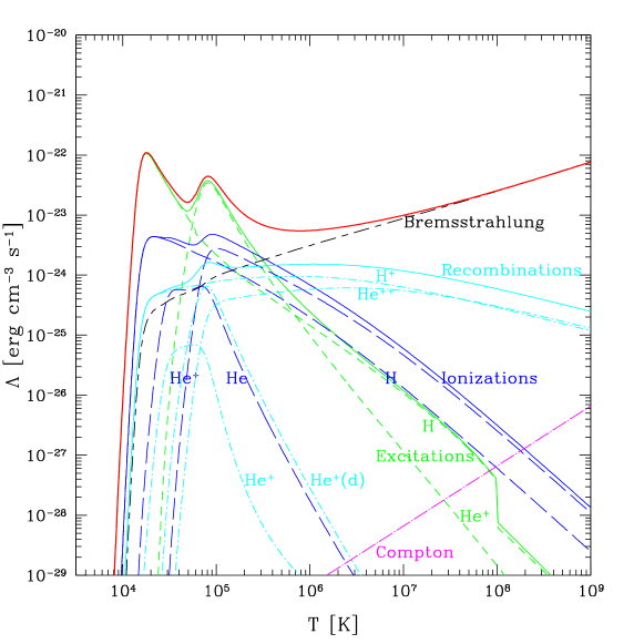
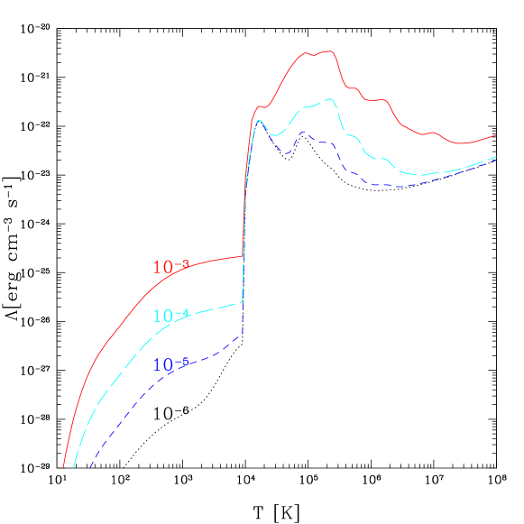
Figure 12: The top panel shows the total cooling curve (solid line) and its composition from different processes for a primordial mixture of H and He. The bottom panel shows how the total cooling curve will change as a function of different metallicity, as indicated in the plot (in absolute values). The part below $10^{4}$ K also takes into account cooling by molecules (e.g. HD and H₂) and metal lines. Taken from Maio et al. (2007).

We discuss here how the $\Lambda(u,\rho)$ term is usually added in the first law of thermodynamics, described by Eq. 49, and its consequences.

In cosmological applications, one is usually interested in structures with virial temperatures larger than $10^{4}$ K. In standard implementations of the cooling function $\Lambda(u,\rho)$, one assumes that the gas is optically thin and in ionisation equilibrium. It is also usually assumed that three-body cooling processes are unimportant, so as to restrict the treatment to two-body processes. For a plasma with primordial composition of H and He, these processes are collisional excitation of H i and He ii, collisional ionisation of H i, He i and He ii, standard recombination of H ii, He ii and He iii, dielectric recombination of He ii, and free-free emission (Bremsstrahlung). The collisional ionisation and recombination rates depend only on temperature. Therefore, in the absence of ionising background radiation one can solve the resulting rate equation analytically. This leads to a cooling function $\Lambda(u)/\rho^{2}$ as illustrated in the top panel of Fig. 12. In the presence of ionising background radiation, the rate equations can be solved iteratively. Note that for a typical cosmological radiation background (e.g. UV background from quasars, see Haardt & Madau 1996), the shape of the cooling function can be significantly altered, especially at low densities. For a more detailed discussion see for example Katz et al. (1996). Additionally, the presence of metals will drastically increase the possible processes by which the gas can cool. As it becomes computationally very demanding to calculate the cooling function in this case, one usually resorts to a pre-computed, tabulated cooling function. As an example, the bottom panel of Fig. 12, at temperatures above $10^{5}$ K, shows the tabulated cooling function by Sutherland & Dopita (1993) for different metallicities of the gas, keeping the ratios of the different metal species fixed to solar values. Note that almost all implementations solve the above rate equations (and therefore the cooling of the gas) as a “sub time step” problem, decoupled from the hydrodynamical treatment. In practice this means that one assumes that the density is fixed across the time step. Furthermore, the time step of the underlying hydrodynamical simulation are in general, for practical reasons, not controlled by or related to the cooling time-scale. The resulting uncertainties introduced by these approximations have not yet been deeply explored and clearly leave room for future investigations.

For the formation of the first objects in haloes with virial temperatures below $10^{4}$ K, the assumption of ionisation equilibrium no longer holds. In this case, one has to follow the non-equilibrium reactions, solving the balance equations for the individual levels of each species during the cosmological evolution. In the absence of metals, the main coolants are H₂ and H${}_{2}^{+}$ molecules (see Abel et al. 1997). HD molecules can also play a significant role. When metals are present, many more reactions are available and some of these can contribute significantly to the cooling function below $10^{4}$ K. This effect is clearly visible in the bottom panel of Fig. 12, for $T<10^{4}$ K. For more details see Galli & Palla (1998) or Maio et al. (2007) and references therein.

4.2 Star formation and feedback

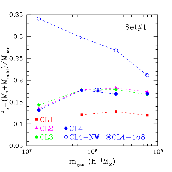
Figure 13: The fraction of cooled baryons $f_{\rm c}$ as a function of the mass of the gas particle, for 4 different clusters at different resolutions is shown. Filled symbols are for the runs including kinetic feedback (e.g. winds), the open circles are re-simulations of one of the clusters with wind feedback turned off. The asterisk is for one of the clusters run at very high resolution using fewer, but 8 times heavier, gas particles than normal, so that the gas particle mass is similar to that of the DM particles in the high–resolution region. Taken from Borgani et al. (2006).

Including radiative losses in simulations causes two numerical problems. Firstly, cooling is a runaway process and, at the typical densities reached at the centres of galaxy clusters, the cooling time becomes significantly shorter than the Hubble time. As a consequence, a large fraction of the baryonic component can cool down and condense out of the hot phase. Secondly, since cooling is proportional to the square of the gas density, its efficiency is quite sensitive to the presence of the first collapsing small halos, where cooling takes place, and therefore on numerical resolution.

To deal with these issues, one has to include in the code a suitable recipe to convert the reservoir of cold and dense gas into collisionless stars. Furthermore, this stellar component should represent the energy feedback from supernova explosions, which ideally would heat the cold gas, so as to counteract the cooling catastrophe.

As for star formation, a relatively simple recipe is that originally introduced by Katz et al. (1996), which is often used in cosmological simulations. According to this prescription, for a gas particle to be eligible to form stars, it must have a convergent flow,

$${\bf{\nabla}}{\bf{v}_{i}}<0\,,$$ (98)

and have density in excess of some threshold value, e.g.

$$\rho_{i}>0.1\ {\rm atoms\,cm}^{-3}.$$ (99)

These criteria are complemented by requiring the gas to be Jeans unstable, that is

$$\frac{h_{i}}{c_{i}}>\frac{1}{\sqrt{4\pi{\rm G}\rho_{i}}}\,,$$ (100)

where $h_{i}$ is either the SPH smoothing length or the mesh size for Eulerian codes and $c_{i}$ is the local sound speed. This indicates that the individual resolution element gets gravitationally unstable. At high redshift, the physical density can easily exceed the threshold given in Eq. 99, even for particles not belonging to virialised halos. Therefore one usually applies a further condition on the gas overdensity,

$$\frac{\rho_{i}}{\rho_{\rm mean}}>55.7,$$ (101)

which restricts star formation to collapsed, virialised regions. Note that the density criterion is the most important one. Particles fulfilling it in almost all cases also fulfill the other two criteria.

Once a gas particle is eligible to form stars, its star formation rate can be written as

$$\frac{\mathrm{d}\rho_{*}}{\mathrm{d}t}=-\frac{\mathrm{d}\rho_{i}}{\mathrm{d}t}=\frac{c_{*}\rho_{i}}{t_{*}}\,,$$ (102)

where $c_{*}$ is a dimensionless star formation rate parameter and $t_{*}$ the characteristic timescale for star formation. The value of this timescale is usually taken to be the maximum of the dynamical time $t_{\rm dyn}=(4\pi{\rm G}\rho_{i})^{-0.5}$ and the cooling time $t_{\rm cool}=u_{i}/(\mathrm{d}u_{i}/\mathrm{d}t)$. In principle, to follow star formation, one would like to produce continuously collisionless star particles. However, for computational and numerical reasons, one approximates this process by waiting for a significant fraction of the gas particle mass to have formed stars according to the above rate; when this is accomplished, a new, collisionless “star” particle is created from the parent star-forming gas particle, whose mass is reduced accordingly. This process takes place until the gas particle is entirely transformed into stars. In order to avoid spurious numerical effects, which arise from the gravitational interaction of particles with widely differing masses, one usually restricts the number of star particles (so called generations) spawned by a gas particle to be relatively small, typically $2-3$. Note that it is also common to restrict the described star-formation algorithm to only convert a gas particle into a star particle, which correspond to the choice of only one generation. In this case star and gas particles have always the same mass.

To get a more continuous distribution of star particle masses, the probability of forming a star can be written as

$$p=1-{\rm exp}\left(-c_{*}\frac{\Delta t}{t_{g}}\right)$$ (103)

and a random number is used to decide when to form a star particle.

According to this scheme of star formation, each star particle can be identified with a Simple Stellar Population (SSP), i.e. a coeval population of stars characterised by a given assumed initial mass function (IMF). Further, assuming that all stars with masses larger than 8 M_⊙ will end as type-II supernovae (SN II), one can calculate the total amount of energy (typically $10^{51}$ erg per supernova) that each star particle can release to the surrounding gas. Under the approximation that the typical lifetime of massive stars which explode as SN II does not exceed the typical time step of the simulation, this is done in the so–called “instantaneous recycling approximation”, with the feedback energy deposited in the surrounding gas in the same step.

Improvements with respect to this model include an explicit sub–resolution description of the multi–phase nature of the interstellar medium, which provides the reservoir of star formation. Such a sub grid model tries to model the global dynamical behaviour of the interstellar medium in which cold, star-forming clouds are embedded in a hot medium.

One example is the multi-phase sub-grid model suggested by Springel & Hernquist (2003), in which a star-forming gas particle has a multi–phase nature, with a cold phase describing cold clouds embedded in pressure equilibrium within a hot medium. According to this model, star formation takes place in a self–regulated way. Within this model (as within other models), part of the feedback energy is channelled back into kinetic energy, effectively leading to a quasi self-consistent modelling of galactic outflows, driven by the star-forming regions. Once an efficient form of kinetic feedback is included, the amount of stars formed in simulations turns out to converge when resolution is varied. An example of the predicted stellar component in different galaxy clusters for varying spatial resolutions, taken from Borgani et al. (2006) is shown in Fig. 13.

A further direction for improvement is provided by a more accurate description of stellar evolution, and of the chemical enrichment associated with star forming particles. More accurate models require that energy feedback and metals are released not just by SN II, but also by SN Ia and low and intermediate mass stars, thereby avoiding the instantaneous recycling approximation (e.g., see Borgani et al. 2008 - Chapter 18, this volume, for a more detailed discussion of this point).

4.3 Additional physics

A number of other physical processes, besides those related to star formation and SN feedback, are in general expected to play a role in the evolution of the cosmic baryons and, as such, should be added into the treatment of the hydrodynamical equations. For instance, magnetic fields or the effect of a population of relativistic particles as described in detail in the review by Dolag et al. 2008 - Chapter 12, this volume. Other processes, whose effect has been studied in cosmological simulations of galaxy clusters include thermal conduction (Jubelgas et al. 2004; Dolag et al. 2004), radiative transfer to describe the propagation of photons in a medium (e.g. Iliev et al. 2006 and references therein), growth of black holes and the resulting feedback associated with the extracted energy (e.g. Sijacki et al. 2007 and references therein. A description of these processes is far outside the scope of this review and we point the interested reader to the original papers cited above.

5 Connecting simulations to observations

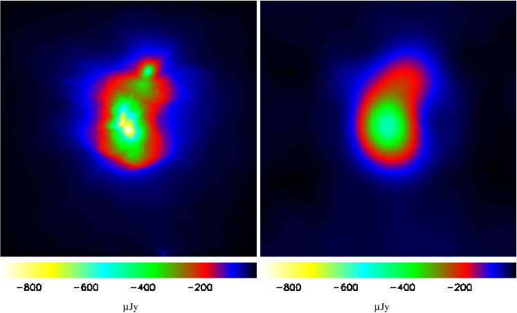
Figure 14: Maps for the SZ decrement for a simulated galaxy cluster. The original map extracted from the hydrodynamic simulation, and the same map in the simulated observation ($t=34$ hour) which assumes the AMI interferometric response, are shown in the left and right panel, respectively. The side of each map corresponds to 16 arcmin. The colour scale is shown at the bottom of each panel. Taken from Bonaldi et al. (2007).

Both the recent generation of instruments and an even more sophisticated next generation of instruments (at various wavelengths) will allow us to study galaxy clusters in rich detail. Therefore, when comparing observations with simulations, instrumental effects like resolution and noise, as well as more subtle effects within the observational processes, have to be taken into account to separate true features from instrumental effects and biases. Therefore, the building up of synthetic instruments to “observe” simulations becomes more and more important.

As an example, Fig. 14 shows the difference between a Sunyaev-Zel’dovich map obtained from a simulated galaxy cluster, and how it would be observed with the AMI instrument, assuming the response according to the array configuration of the radio dishes and adding the appropriate noise. Here a $34$ hour observation has been assumed, and the CLEAN deconvolution algorithm applied. For details see Bonaldi et al. (2007).

Another example of a synthetic observation by a virtual telescope is shown in Fig. 15, which shows an optical image of a simulated galaxy cluster with several strong lensing features. Here, Meneghetti et al. (2007) investigated the capability of the planned DUNE mission to measure the properties of gravitational arcs, including instrumental effects as well as the disturbance by light from the cluster galaxies. Shapelet decompositions - based on galaxy images retrieved from the GOODS-ACS archive - were used to describe the surface brightness distributions of both the cluster members and the background galaxies. For the cluster members the morphological classifications inferred from the semi-analytic modelling, based on the merger tree of the underlying cluster simulations were used to assign a spectral energy distribution to each. Several sources of noise like photon noise, sky background, seeing, and instrumental noise are included. For more details see Meneghetti et al. (2007).

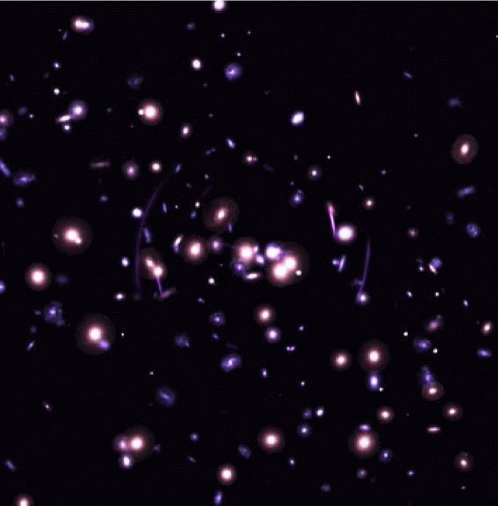
Figure 15: Composite $ugr+riz+izy$ image of a simulated galaxy cluster including its simulated lensing signal, having its imprint in several strong lensing features. To construct the surface brightness distributions of both the cluster members and of the background galaxies, shapelet decompositions were used. For each cluster galaxy the morphological classifications and spectral energy distribution inferred from the semi-analytic modelling based on the merger trees from the underlying cluster simulation were used to realistically model the optical appearance of the cluster. The field of view is $100^{\prime\prime}\times 100^{\prime\prime}$ and an exposure of 1000 s for each band was assumed. Taken from Meneghetti et al. (2007).

Thanks to its high temperature (around $10^{8}$ K) and its high density (up to $10^{-3}$ particles per cm³) the intra-cluster medium is an ideal target to be studied by X-ray telescopes. Therefore, so far, most effort towards understanding systematic in the observational process of galaxy clusters has been spent interpreting X-ray observations.

For a direct comparison of the simulations with X-ray observations one has to calculate from the simulated physical quantities (density, temperature, $\ldots$) the observed quantities (e.g. surface brightness). The other way – going from observations to physical quantities – is much more difficult and would require a number of assumptions. Fortunately, the ICM is usually optically thin, so that absorption of photons within the ICM does not have to be taken into account. Hence to obtain an X-ray image of the modelled cluster, one has to choose a projection direction and integrate over all the emission of the elements along the line of sight for each pixel in the image. The X-ray emission at each element is usually approximated as the product of the square of the density and the cooling function. As X-ray detectors are only sensitive in a certain energy range, one must be careful to take the correct range. For very realistic images one needs to taken into account also the effects of the X-ray telescopes and detectors (e.g. the limited resolution of the X-ray telescope (point spread function) or the energy and angle dependent sensitivy (detector response matrix and vignetting). As observed images also depend on the distance of the cluster and the (frequency dependent) absorption of the X-ray emission in the Galaxy these should also be accounted for. For an exact prediction, the emitted spectrum of each element has to be taken into account, as well as many of the effects mentioned above are energy dependent.

Even more difficult is the comparison of quantities derived from spectral analyses such as ICM temperature and ICM metallicity, or their projections in profiles and maps. A pixel in an observed temperature map, for example, is derived using all the photons within the pixel area, and the derived spectrum is fitted with a single model of a hot plasma (see Kaastra et al. 2008 - Chapter 9, this volume). These photons, however, come from different positions along the line of sight, that have different emissivities, different temperature and different metallicities. So the spectrum is actually a composite of many different spectra. Obviously such a multi-temperature spectrum cannot be fitted very well by a single temperature model. Sometimes temperature maps are produced in an even cruder way using the ratio of two or more energy bands. These are called hardness ratio maps.

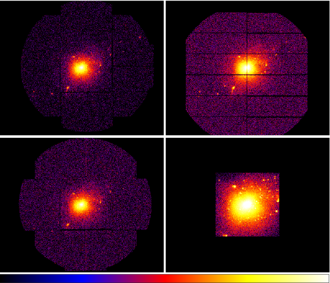
Figure 16: Simulated photon images in the $0.7-2$ keV energy band of a simulated galaxy cluster using XMAS-2. The images are binned to 3.2 arcsec. They include background, vignetting effects, out-of-time events and the telescope optical paths. From top left to bottom right are simulations for the MOS1, PN, and MOS2 instruments on board of the XMM-Newton satellite and for the ACIS-S3 instrument onboard of the Chandra satellite. Kindly provided by Elena Rasia, see Rasia et al. (2006) and Rasia et al. (2007).

To calculate temperatures, temperature profiles or temperature maps are calculated using mostly emission weighted temperatures, i.e. summing the temperature of all elements along the line of sight, weighted by their emission

$$T={\int WT\mathrm{d}V\over\int W\mathrm{d}V}$$ (104)

with $T$ being the gas temperature and $W$ a weighting factor. Usually $W$ is proportional to the emissivity of each gas element,

$$W=\Lambda(T)n^{2}$$ (105)

where $\Lambda(T)$ is the cooling curve and $n$ the gas density.

This simple procedure does not of course take into account the shape of the spectra corresponding to gas of different temperatures. It therefore gives only a rough estimate of the actual temperature. With numerical simulations it was investigated how accurate these emission weighted temperatures are, by comparing them with temperatures obtained by actually adding spectra, so-called spectroscopic temperatures. It was found that the emission-weighted temperatures are systematically higher than the spectroscopic temperatures (Mathiesen & Evrard 2001; Gardini et al. 2004; Mazzotta et al. 2004). To overcome this problem, Mazzotta et al. (2004) suggested an approximation to the spectroscopic temperature, the “spectroscopic-like” temperature $T_{\rm sl}$

$$T_{\rm sl}={\int n^{2}T^{\alpha}/T^{1/2}\mathrm{d}V\over\int n^{2}T^{\alpha}/T^{3/2}\mathrm{d}V}$$ (106)

which yields for $\alpha=0.75$ a good estimate of the spectroscopic temperature. In addition the simulated $M$-$T$ relation is strongly affected, if the emission-weighted temperature is used (Rasia et al. 2005).

The inhomogenous temperature and metal distribution was also found to be responsible also for inaccurate metallicity measurements. Rasia et al. (2007) studied with numerical simulations, together with the programme X-MAS2, how well the elements Fe, O, Mg and Si can be measured in clusters of different temperature. They find that Fe and Si are generally measureable with good accuracy, while O and Mg can be considerably overestimated in hot clusters. Using simulations and the programme SPEX (see Kaastra et al. 2008 - Chapter 9 this volume) Kapferer et al. (2007) found that due to the metal inhomogeneities the metal mass in clusters is systematically underestimated – in extreme cases by up to a factor of three.

An example of synthetic X-ray observations is shown in Fig. 16. Here XMAS-2 is used to produce photon images from a simulated galaxy cluster. Shown are simulations for the MOS1, PN, and MOS2 instruments on board the XMM-Newton satellite, and for the ACIS-S3 instrument on board the Chandra satellite. They include instrumental effects like background, vignetting and response for the individual instruments. For more details see Rasia et al. (2006) and Rasia et al. (2007).

6 Outlook

In the future, the demand on precision in both simulation techniques and captured complexity of the physical processes within the simulations will be quite challenging. Recent leading simulations are already extremely difficult to analyse due to their enormous size and complexity, and they will surely continue to grow. In fact, the next generation of supercomputers will grow more in the number of accessable CPUs than on the speedup of the individual CPUs and this fact will make the analysis of the simulations as challenging as performing the simulations itself. To keep a comparable level of accuracy, the interpretation of a simulation of the next generation of high precision experiments will need to massively involve virtual telescopes as described in the previous section. This will increase the need of involving complex analysis pipelines for “observing” simulations, and might lead to a new branch of virtual observers in the astrophysics community, similar to the already, new formed branch of computational astrophysicists.

7 Acknowledgments

The authors thank ISSI (Bern) for support of the team “Non-virialized X-ray components in clusters of galaxies”. Special thanks to Volker Springel for helping to improve the manuscript and providing Fig. 7 to Anna Watts for carefully reading the manuscript, to Martin Obergaulinger for very helpful discussions on Eulerian schemes, to Ewald Müller for the lecture notes on the Riemann problem and providing Fig. 10, to Elena Rasia for providing Fig. 16 and to Umberto Maio for providing Fig. 12. A.D. also gratefully acknowledges partial support from the PRIN2006 grant “Costituenti fondamentali dell’Universo” of the Italian Ministry of University and Scientific Research and from the INFN grant PD51.

References

- Abel et al. (1997) Abel, T., Anninos, P., Zhang, Y., & Norman, M. L. 1997, New Astronomy, 2, 181
- Agertz et al. (2007) Agertz, O., Moore, B., Stadel, J., et al. 2007, MNRAS, 380, 963
- Athanassoula et al. (1998) Athanassoula, E., Bosma, A., Lambert, J.-C., & Makino, J. 1998, MNRAS, 293, 369
- Bagla (2002) Bagla, J. S. 2002, J. Astroph. Astron., 23, 185
- Bagla & Ray (2003) Bagla, J. S. & Ray, S. 2003, New Astronomy, 8, 665
- Balsara (1995) Balsara, D. S. 1995, J. Comp. Phys., 121, 357
- Bardeen et al. (1986) Bardeen, J. M., Bond, J. R., Kaiser, N., & Szalay, A. S. 1986, ApJ, 304, 15
- Barnes & Hut (1986) Barnes, J. & Hut, P. 1986, Nature, 324, 446
- Bertschinger (1995) Bertschinger, E. 1995, COSMICS: Cosmological initial conditions and microwave anisotropy codes (astro-ph/9506070)
- Bode et al. (2000) Bode, P., Ostriker, J. P., & Xu, G. 2000, ApJS, 128, 561
- Bonaldi et al. (2007) Bonaldi, A., Tormen, G., Dolag, K., & Moscardini, L. 2007, MNRAS, 378, 1248
- Borgani et al. (2006) Borgani, S., Dolag, K., Murante, G., et al. 2006, MNRAS, 367, 1641
- Borgani et al. (2008) Borgani, S., Fabjan, D., Tornatore, L., et al. 2008, SSR, in press
- Bryan et al. (1995) Bryan, G. L., Norman, M. L., Stone, J. M., Cen, R., & Ostriker, J. P. 1995, Comp. Phys. Commun., 89, 149
- Cen (1992) Cen, R. 1992, ApJS, 78, 341
- Chapra & Canale (1997) Chapra, S. C. & Canale, R. P. 1997, Numerical Methods for Engineers: With Programming and Software Applications (McGraw-Hill, New York)
- Colella & Glaz (1985) Colella, P. & Glaz, H. M. 1985, J. Comp. Phys., 59, 264
- Colella & Woodward (1984) Colella, P. & Woodward, P. R. 1984, J. Comp. Phys., 54, 174
- Couchman (1991) Couchman, H. M. P. 1991, ApJ, 368, L23
- Couchman et al. (1995) Couchman, H. M. P., Thomas, P. A., & Pearce, F. R. 1995, ApJ, 452, 797
- Courant & Friedrichs (1948) Courant, R. & Friedrichs, K. O. 1948, Supersonic flow and shock waves (Interscience, New York)
- Dehnen (2000) Dehnen, W. 2000, ApJ, 536, L39
- Dolag et al. (2008) Dolag, K., Bykov, A. M., & Diaferio, A. 2008, SSR, in press
- Dolag et al. (2004) Dolag, K., Jubelgas, M., Springel, V., Borgani, S., & Rasia, E. 2004, ApJ, 606, L97
- Dolag et al. (2005) Dolag, K., Vazza, F., Brunetti, G., & Tormen, G. 2005, MNRAS, 364, 753
- Efstathiou et al. (1985) Efstathiou, G., Davis, M., White, S. D. M., & Frenk, C. S. 1985, ApJS, 57, 241
- Einfeldt (1988) Einfeldt, B. 1988, 25, 294
- Einfeldt et al. (1991) Einfeldt, B., Roe, P. L., Munz, C. D., & Sjogreen, B. 1991, J. Comp. Phys., 92, 273
- Ettori et al. (2006) Ettori, S., Dolag, K., Borgani, S., & Murante, G. 2006, MNRAS, 365, 1021
- Evrard (1988) Evrard, A. E. 1988, MNRAS, 235, 911
- Evrard et al. (2002) Evrard, A. E., MacFarland, T. J., Couchman, H. M. P., et al. 2002, ApJ, 573, 7
- Feng et al. (2004) Feng, L.-L., Shu, C.-W., & Zhang, M. 2004, ApJ, 612, 1
- Frenk et al. (1999) Frenk, C. S., White, S. D. M., Bode, P., et al. 1999, ApJ, 525, 554
- Fryxell et al. (2000) Fryxell, B., Olson, K., Ricker, P., et al. 2000, ApJS, 131, 273
- Fukushige et al. (1991) Fukushige, T., Ito, T., Makino, J., et al. 1991, PASJ, 43, 841
- Galli & Palla (1998) Galli, D. & Palla, F. 1998, A&A, 335, 403
- Gardini et al. (2004) Gardini, A., Rasia, E., Mazzotta, P., et al. 2004, MNRAS, 351, 505
- Gingold & Monaghan (1977) Gingold, R. A. & Monaghan, J. J. 1977, MNRAS, 181, 375
- Haardt & Madau (1996) Haardt, F. & Madau, P. 1996, ApJ, 461, 20
- Harten (1983) Harten, A. 1983, J. Comp. Phys., 49, 357
- Harten et al. (1987) Harten, A., Engquist, B., Osher, S., & Chakravarthy, S. R. 1987, J. Comp. Phys., 71, 231
- Harten et al. (1983) Harten, A., Lax, P. D., & van Leer, B. 1983, 25, 35
- Heitmann et al. (2007) Heitmann, K., Lukic, Z., Fasel, P., et al. 2007, report LA-UR-07-1953 (astro-ph/0706.1270)
- Hernquist (1993) Hernquist, L. 1993, ApJ, 404, 717
- Hernquist & Katz (1989) Hernquist, L. & Katz, N. 1989, ApJS, 70, 419
- Hockney & Eastwood (1988) Hockney, R. W. & Eastwood, J. W. 1988, Computer simulation using particles (Hilger, Bristol)
- Hut et al. (1995) Hut, P., Makino, J., & McMillan, S. 1995, ApJ, 443, L93
- Iliev et al. (2006) Iliev, I. T., Ciardi, B., Alvarez, M. A., et al. 2006, MNRAS, 371, 1057
- Ito et al. (1993) Ito, T., Makino, J., Fukushige, T., et al. 1993, PASJ, 45, 339
- Jiang & Shu (1996) Jiang, G.-S. & Shu, C.-W. 1996, J. Comp. Phys., 126, 202
- Jubelgas et al. (2004) Jubelgas, M., Springel, V., & Dolag, K. 2004, MNRAS, 351, 423
- Kaastra et al. (2008) Kaastra, J. S., Paerels, F. B. S., Durret, F., Schindler, S., & Richter, P. 2008, SSR, in press
- Kang et al. (1994) Kang, H., Ostriker, J. P., Cen, R., et al. 1994, ApJ, 430, 83
- Kapferer et al. (2007) Kapferer, W., Kronberger, T., Weratschnig, J., & Schindler, S. 2007, A&A, 472, 757
- Katz et al. (1996) Katz, N., Weinberg, D. H., & Hernquist, L. 1996, ApJS, 105, 19
- Kawai et al. (2000) Kawai, A., Fukushige, T., Makino, J., & Taiji, M. 2000, PASJ, 52, 659
- Kravtsov (2002) Kravtsov, A. 2002, APS Meeting Abstracts (/http://flux.aps.org/meetings/YR02/APR02/ baps/abs/S820004.html)
- Kravtsov et al. (1997) Kravtsov, A. V., Klypin, A. A., & Khokhlov, A. M. 1997, ApJS, 111, 73
- Kravtsov et al. (2005) Kravtsov, A. V., Nagai, D., & Vikhlinin, A. A. 2005, ApJ, 625, 588
- LeVeque (2002) LeVeque, R. 2002, Finite volume methods for hyperbolic problems, Cambridge texts in applied mathematics (Cambridge University Press)
- Levy et al. (1999) Levy, D., Puppo, G., & Russo, G. 1999, Berkeley CPAM 762 (arXiv:math/9911089)
- Li (2005) Li, S. 2005, J. Comp. Phys., 203, 344
- Li et al. (2006) Li, S., Li, H., & Cen, R. 2006, ApJS, submitted (astro-ph/0611863)
- Lucy (1977) Lucy, L. B. 1977, AJ, 82, 1013
- Maio et al. (2007) Maio, U., Dolag, K., Ciardi, B., & Tornatore, L. 2007, MNRAS, 379, 963
- Makino (1991) Makino, J. 1991, PASJ, 43, 621
- Mathiesen & Evrard (2001) Mathiesen, B. F. & Evrard, A. E. 2001, ApJ, 546, 100
- Mazzotta et al. (2004) Mazzotta, P., Rasia, E., Moscardini, L., & Tormen, G. 2004, MNRAS, 354, 10
- Meneghetti et al. (2007) Meneghetti, M., Melchior, P., Grazian, A., et al. 2007, A&A, submitted (astro-ph/0711.3418)
- Monaghan (1992) Monaghan, J. J. 1992, ARAA, 30, 543
- Monaghan (1997) Monaghan, J. J. 1997, J. Comp. Phys., 136, 298
- Monaghan & Gingold (1983) Monaghan, J. J. & Gingold, R. A. 1983, J. Comp. Phys., 52, 374
- Morris & Monaghan (1997) Morris, J. P. & Monaghan, J. J. 1997, J. Comp. Phys., 136, 41
- Navarro & White (1993) Navarro, J. F. & White, S. D. M. 1993, MNRAS, 265, 271
- O’Shea et al. (2005) O’Shea, B. W., Nagamine, K., Springel, V., Hernquist, L., & Norman, M. L. 2005, ApJS, 160, 1
- Owen et al. (1998) Owen, J. M., Villumsen, J. V., Shapiro, P. R., & Martel, H. 1998, ApJS, 116, 155
- Peebles (1980) Peebles, P. J. E. 1980, The large-scale structure of the universe (Princeton Univ. Press)
- Pen (1998) Pen, U.-L. 1998, ApJS, 115, 19
- Powell et al. (1999) Powell, K. G., Roe, P. L., Linde, T. J., Gombosi, T. I., & de Zeeuw, D. L. 1999, J. Comp. Phys., 154, 284
- Power et al. (2003) Power, C., Navarro, J. F., Jenkins, A., et al. 2003, MNRAS, 338, 14
- Press et al. (1992) Press, W. H., Teukolsky, S. A., Vetterling, W. T., & Flannery, B. P. 1992, Numerical recipes in FORTRAN. The art of scientific computing (2nd ed., Cambridge Univ. Press)
- Quinn et al. (1997) Quinn, T., Katz, N., Stadel, J., & Lake, G. 1997, ApJ, submitted but not published (astro-ph/9710043)
- Rasia et al. (2006) Rasia, E., Ettori, S., Moscardini, L., et al. 2006, MNRAS, 369, 2013
- Rasia et al. (2005) Rasia, E., Mazzotta, P., Borgani, S., et al. 2005, ApJ, 618, L1
- Rasia et al. (2007) Rasia, E., Mazzotta, P., Bourdin, H., et al. 2007, ApJ, in press (astro-ph/0707.2614)
- Ricker et al. (2000) Ricker, P. M., Dodelson, S., & Lamb, D. Q. 2000, ApJ, 536, 122
- Ryu et al. (1993) Ryu, D., Ostriker, J. P., Kang, H., & Cen, R. 1993, ApJ, 414, 1
- Schive et al. (2007) Schive, H.-Y., Chien, C.-H., Wong, S.-K., Tsai, Y.-C., & Chiueh, T. 2007, New Astron., submitted (astro-ph/0707.2991)
- Shu (1998) Shu, C.-W. 1998, in Advanced numerical approximate of nonlinear hyperbolic equations. Lecture notes in mathematics 1697, ed. A. Quarteroni (Springer), 285
- Sijacki et al. (2007) Sijacki, D., Springel, V., di Matteo, T., & Hernquist, L. 2007, MNRAS, 380, 877
- Silverman (1986) Silverman, B. W. 1986, Density estimation for statistics and data analysis (Monographs on statistics and applied probability, Chapman and Hall, London)
- Springel (2005) Springel, V. 2005, MNRAS, 364, 1105
- Springel & Hernquist (2002) Springel, V. & Hernquist, L. 2002, MNRAS, 333, 649
- Springel & Hernquist (2003) Springel, V. & Hernquist, L. 2003, MNRAS, 339, 289
- Springel et al. (2001a) Springel, V., White, M., & Hernquist, L. 2001a, ApJ, 549, 681
- Springel et al. (2001b) Springel, V., Yoshida, N., & White, S. D. M. 2001b, New Astron., 6, 79
- Steinmetz (1996a) Steinmetz, M. 1996a, MNRAS, 278, 1005
- Steinmetz (1996b) Steinmetz, M. 1996b, in IAU Symp. 171: New light on galaxy evolution, 259
- Stoehr et al. (2003) Stoehr, F., White, S. D. M., Springel, V., Tormen, G., & Yoshida, N. 2003, MNRAS, 345, 1313
- Stone & Norman (1992) Stone, J. M. & Norman, M. L. 1992, ApJS, 80, 753
- Sutherland & Dopita (1993) Sutherland, R. S. & Dopita, M. A. 1993, ApJS, 88, 253
- Tormen et al. (1997) Tormen, G., Bouchet, F. R., & White, S. D. M. 1997, MNRAS, 286, 865
- White (1996) White, S. D. M. 1996, in Cosmology and large scale structure, ed. R. Schaeffer, J. Silk, M. Spiro, & J. Zinn-Justin, 349
- Xu (1995) Xu, G. 1995, ApJS, 98, 355
- Zel’dovich (1970) Zel’dovich, Y. B. 1970, A&A, 5, 84