An implicit numerical algorithm for solving the general relativistic hydrodynamical equations around accreting compact objects

Abstract

An implicit algorithm for solving the equations of general relativistic hydrodynamics in conservative form in three-dimensional axi-symmetry is presented. This algorithm is a direct extension of the pseudo-Newtonian implicit radiative magnetohydrodynamical solver -IRMHD- into the general relativistic regime.

We adopt the Boyer-Lindquist coordinates and formulate the hydrodynamical equations in the fixed background of a Kerr black hole. The set of equations are solved implicitly using the hierarchical solution scenario (HSS). The HSS is efficient, robust and enables the use of a variety of solution procedures that range from a purely explicit up to fully implicit schemes. The discretization of the HD-equations is based on the finite volume formulation and the defect-correction iteration strategy for recovering higher order spatial and temporal accuracies. Depending on the astrophysical problem, a variety of relaxation methods can be applied. In particular the vectorized black-white Line-Gauss-Seidel relaxation method is most suitable for modeling accretion flows with shocks, whereas the Approximate Factorization Method is for weakly compressible flows.

The results of several test calculations that verify the accuracy and robustness of the algorithm are shown. Extending the algorithm to enable solving the non-ideal MHD equations in the general relativistic regime is the subject of our ongoing research.

, and

1 Introduction

The field of astrophysical fluid dynamics (henceforth AFD) deals with the macroscopic evolution of gaseous-matter and plasmas in a wide variety of circumstances in astrophysics. The scope of AFD is broad, encompassing topics such as star formation, accretion phenomena onto compact and young stellar objects, dynamics of the interstellar medium, jets, winds and outflows emerging from around young stellar objects, from quasars and microquasars, supernovae explosion, $\gamma-$ray bursts and structure formation in the universe.

One of the ultimate aims of numerical astrophysics is to develop a black box algorithm which contains numerical solvers that are unconditionally stable, robust, efficient, Newtonian, relativistic and capable of treating flows that are strongly compressible, weakly incompressible, self-gravitating, radiating, magnetized multi-component-plasmas with high spatial and temporal accuracies on unstructured meshes and to provide the required solutions within the scale of hours. While this goal is unlikely to be achieved within the next few years, the increasing number of sophisticated numerical algorithms developed during the last two decades is remarkably encouraging. In particular, significant improvements have been achieved in increasing the spatial dimensions and enhancing the efficiency and accuracy of numerical algorithms (see e.g. Nagel et al., 2006).
On the other hand, the problem of robustness of the solvers in AFD has been barely considered nor even seriously discussed. In this paper we discuss the robustness problem in AFD, present enhancement strategies and address the necessity of constructing robust general relativistic implicit and radiative MHD solvers. For completeness we review the concepts of efficiency and robustness of numerical solvers in computational fluid dynamics.

A numerical solver is said to be relatively efficient if the corresponding number of algebraic manipulations per time step per computer-processor can be made respectively small. As a consequence, using high performance computers with large number of computing processors, a significant progress has been achieved in improving runtime efficiencies, provided the computing load is distributed appropriately. Thus, by means of modern hardware technology, the efficiency of computer-codes could be enhanced even without modifying the employed mathematical approach. This has led to uncoordinated developments of relatively large number of computer-codes, that may differ in efficiency and integrated physical processes but are almost essentially identical with respect to the mathematical solution procedure. This phenomenon can be attributed to the lack of robustness. By robustness, we mean the capability of a solver to be applied to a large class of problems without modifying the algorithmic core significantly.

In an attempt to enhance both efficiency and robustness, the hierarchical solution strategy (HSS) has been suggested (Fig. 1 and 2, also see Hujeirat (2005) and the references therein). The HSS relies on the fact that any set of hydrodynamical, magnetohydrodynamical or radiative equations are linearize-able and therefore can be re-written in a simple matrix equation $Aq=b,$ where $A,q,b$ are the coefficient matrix, vector of unknown variables and the vector of known quantities, respectively. Applying the defect-correction strategy (Stetter, 1978; Böhmer, Stetter, 1984), we may then re-write this equation as: $A\delta q=d,$ where $\delta q$ and $d$ denote respectively the vectors of small-time corrections and the defect, provided $d$ is consistent with the real mathematical equations by construction. The matrix A in the latter equation can be replaced by a variety of matrices that correspond to a sequence of numerical approaches that ranges from purely explicit to strongly implicit (Hujeirat, 2005). In this formulation, explicit methods arise as a special case, in which A is being replaced by the most easiest invertible-matrix: the identity matrix I. Based on this formulation, the Courant condition follows from the requirement that the matrix A should be stable-invertible.

Therefore, strongly implicit and explicit methods are different variants of the same algebraic problem. While the former retain almost all the entries of the matrix A in the inversion procedure, the latter rely on neglecting all off-diagonal entries as well as crudely simplifying the diagonal elements. These methods are well-unified within the HSS, and that depending on the physical properties of the flow, a directive will carefully select the entries of A that are relevant for the problem.

In Table 1 we have summarized properties of several numerical methods. Thus, as long as efficiency is concerned, explicit methods are unrivalled candidates, provided the flows are strongly time-dependent and compressible. However, due to the relatively large sound speed, these methods may stagnate both in modeling incompressible or even weakly compressible flows. To clarify this point, we mention that the time step-size in explicit methods must satisfy the Courant-Friedrichs-Lewy (CFL) condition:

$$\delta t_{exp}<\min\{\frac{\Delta x}{U+V_{s}}\}=\min\{\frac{\Delta x}{U(1+1/\cal{M})}\},$$

where the minimum function runs over all points of the domain of calculation. Here $\delta t_{exp},\Delta x,U,V_{s},\cal{M}$ correspond to the explicit time step-size, space increment, velocity, sound speed and the Mach number, respectively. Therefore, as ${\cal{M}}\rightarrow 0$ the flow becomes incompressible and the time step size approaches zero; hence a stagnation of the time-advancement procedure. We note that although in this case using consistent implicit solution procedures is necessary, by no means it is sufficient. Here it has been verified that standard implicit solvers experience serious difficulties in simulating low Mach number flows, typically found in the interior layers of stars, planets as well as around moving vehicles in the Earth atmosphere.

The above discussion addresses the following questions: 1) Relativistic fluid motions typically occur on the dynamical time scale. The advantages of still using implicit solvers should be clarified. 2) Multigrid methods have been shown to display convergence which depends weakly on the number of unknowns in the finite space. In combination with nested iteration, the multigrid method can solve these problems to truncation error accuracy in a number of operations that is proportional to the number of unknowns. Therefore the reason for still favouring the prolongation strategy over multigrid or adaptive mesh refinement needs to be explained. 3) The storage capacities of modern computers to date are capable of handling the entries of large matrices that correspond to the 3D MHD equations. Thus, the reliability and credibility of 3D axi-symmetric algorithms should be justified.

In fact, there are several reasons that justify using implicit numerical procedures for modeling relativistic flows. In particular:

• The set of relativistic MHD equations is generically a highly coupled non-linear system, which gives rise to fast growing perturbations due to non-linearities, thereby imposing a further restriction on the size of the time step.

• In most of the cases the horizon of a black hole represents a geometrical singularity. The deformation of the geometry grows non-linearly when approaching the black hole. Thus, in order to capture flow-configurations in the vicinity of a black hole accurately, a non-linear distribution of the grid points is necessary, which, again, may destabilize explicit schemes.

• Depending on the evolutionary conditions, non-relativistic flows may become ultra-relativistic or vice versa. However, almost all non-relativistic astrophysical flows known to date are considered to be dissipative and diffusive. Therefore, in order to track their time-evolution reliably, the employed numerical solver should be capable of treating the corresponding second order viscous terms properly.

• The timescales of most astrophysical flows are considered to have a great disparity. Stability requirement of conditionally stable methods however requires that the time step size should be a small fraction of the shortest possible timescale. This implies that, in order to cover a timescale of astrophysical relevance, an extremely large number of time steps would be required, which would give rise to prohibitive computational costs. Furthermore, the accumulated round off errors resulting from performing a large number of time-extrapolations for time-advancing a numerical hydrodynamical solution may easily cause divergence.

• The initial conditions of most astrophysical phenomena are not known. Therefore, in carrying out global hydrodynamical simulations, the end solution should weakly depend on the initial flow configuration. Conditionally stable numerical methods, however, rely on time-advancing of the initial conditions.

The latter reason may explain also why using the prolongation strategy is advantageous over classical multigrid. Worth noting is that the main building blocks of multigrid methods are:

1. Restriction, i.e., down sampling of the residual errors into coarser meshes.

2. Residual smoothing: reducing the high frequency errors by performing several iterations, using a computationally efficient iterative procedure such as Jacobi or Gauss-Seidel.

3. Prolongation, which relies on the interpolation from the coarse onto finer meshes.

The high-frequency errors here are reduced by cheap smoothing on the fine meshes, whereas the low-frequency errors are reduced by defect correction on the coarser meshes. As the bulk of the algebraic operations are made on the coarser meshes, the combined solution procedure is considerably efficient. However, multigrid methods display satisfactory convergence, if the underlying flows are predominantly diffusion-dominated. In the case of advection-dominated flows, errors, that are responsible for the slow convergence on the fine meshes, can be easily advected by the flow on the coarser meshes, thereby reducing the coarse grid correction. In the case of astrophysical flows, the corresponding equations may change their character from Newtonian into ultra-relativistic or vice versa. Unlike Newtonian flows that are generically diffusion-dominated, relativistic flows may become predominantly advection-dominated, depending on how large the corresponding Lorentz factors are. Hence, multigrid methods may fail to provide the expected rate of convergence.

Finally we note that in order to model the formation and acceleration of relativistic flows in the vicinity of ultra-compact objects accurately, it is necessary to cover the domain of calculation by a strongly stretched mesh. Furthermore, Lorentz factors enhance the inner-coupling of the relativistic equations and give rise to a larger spectrum of non-linearities. These numerical difficulties combined with the need to include sophisticated magnetic and radiative processes make the construction of a fully 3D algorithm, at the moment, a computationally unrealizable numerical task.

Therefore, in this paper, we do not intend to perform 3D global simulations, but rather focus on the algorithmic structure of unconditionally stable and robust 3D axi-symmetric solvers. These algorithms should enable us to search for stationary or quasi-stationary solutions for the fully-coupled radiative MHD equations in which detailed physical processes are taken into account.
The paper runs as follows: in Sec. 2 we describe the relativistic hydrodynamical equations, in Sec. 3 the transformation between the primitive and conservative variables is described. The numerical solution and the discretization methods are presented in Sections 4 and 5. In Sec. 6 we present the results of several test calculations and end up with a summary in Sec. 7.

	Explicit	Implicit	HSS
solution method	$q^{n+1}=q^{n}+\delta t\,d^{n}$	$q^{n+1}=q^{n}+\delta t\tilde{A}^{-1}d^{*}$	$q^{n+1}=\alpha q^{n}+(1-\alpha)\delta t\tilde{A}_{d}^{-1}d^{*}$
Type of flows	Strongly time- dependent, compressible, weakly dissipative HD and MHD in 1, 2 and 3 dimensions	Stationary, quasi-stationary, highly dissipative, radiative and axi-symmetric MHD-flows in 1, 2 and 3 dimensions	Stationary, quasi-stationary, weakly compressible, highly dissipative, radiative and axi-symmetric MHD-flows in 1, 2 and 3 dimensions
Stability	conditioned	unconditioned	unconditioned
Efficiency	$1$ (normalized/2D)	$\sim m^{2}$	$\sim m_{d}^{2}$
Efficiency: Enhancement strategies	Parallelization	Parallelization, preconditioning, multigrid	HSS, parallelization, preconditioning, prolongation
Robustness: Enhancement strategies	i. subtime-stepping ii. stiff terms are solved semi-implicitly	i. multiple iteration ii. reducing the time step size	i. multiple iteration ii. reducing the time step size, HSS
Numerical Codes Newtonian	Solvers1a ZEUS&ATHENAb, FLASHc, NIRVANAd, PLUTOe, VACf	Solver2g	IRMHDh
Numerical Codes Relativistic	Solvers3i GRMHDj, ENZOk, PLUTOl, HARMm, RAISHINn, RAMo, GENESISp, WHISKYq	Solver4r	GR-I-RMHDs

Table 1: A list of only a part of the grid-oriented codes in AFD and their range of applications. The matrix-equations in the first row are illustrated in Sec. 4. In these equations, $q^{n,n+1}$, ${\delta t}$, ${\tilde{A}}$, $\alpha$ and $d^{*}$ denote the vector of variables from the old and new time levels, time step size, a preconditioning matrix, a switch on/off parameter and a time-modified defect vector, respectively. “m” in row 4 denotes the bandwidth of the corresponding matrix.

  ^aBodenheimer et al. (1978); Clarke (1996), ^bStone, Norman (1992); Gardiner, Stone (2006), ^cFryxell et al. (2000), ^dZiegler (1998), ^eMignone, Bodo (2003); Mignone et al. (2007), ^fTóth et al. (1998), ^gWuchterl (1990); Swesty (1995), ^hHujeirat (1995, 2005); Falle (2003), ⁱKoide et al. (1999); Komissarov (2004); Anninos et al. (2005); Meliani et al. (2007); Del Zanna et al. (2007), ^jDe Villiers, Hawley (2003), ^kWang et al. (2007), ^lMignone et al. (2007), ^mGammie et al. (2003), ⁿMizuno et al. (2006), ^oZhang, MacFadyen (2006), ^pAlay et al. (1999), ^qBaiotti et al. (2003), ^rLiebendörfer et al. (2002), ^sthe present algorithm.

2 The hydrodynamical equations in Kerr spacetime

In the present study we intend to numerically solve the equations of hydrodynamics in both ultra-relativistic and purely Newtonian regimes. Unlike the usual convention, in which the speed of light and the gravitational constant are set to unity, we use the sound speed as the basic measure for velocities. This is reasonable as the radial motion of rotating flows around a compact object can be as low as $10^{-5\pm 1}$ the speed of light, whereas it is $10^{-2\pm 1}$ of the sound speed. Close to the event horizon, all velocities become quantitatively comparable. This scaling enables the present algorithm to capture the structure of slow flows accurately and renders the appearance of terms that are extremely large or small due to scaling effects. Additionally, the present solution procedure is actually an extension of the purely Newtonian solver, IRMHD, into the general relativistic regime.

2.1 The metric

For completeness, we develop here the equations of hydrodynamics in the background of spacetime metric of a Kerr black hole, using the Boyer-Lindquist coordinates ($t$, $r$, $\theta$, $\phi$). Adopting the 3+1 split of spacetime, a line element with the metric signature $(-,+,+,+)$ can be written as follows:

$$ds^{2}=-\alpha^{2}dt^{2}+h_{\mathrm{ik}}(dx^{i}+\beta^{i}dt)(dx^{k}+\beta^{k}dt),\,\,\textrm{for j,k=1, 3}.$$ (1)

For the Kerr metric, the line element reads:

$$ds^{2}=-(\alpha^{2}-\beta_{\phi}\beta^{\phi})dt^{2}+2\beta_{\phi}d\phi dt+h_{\mathrm{ik}}dx^{i}dx^{k},$$ (2)

which corresponds to a matrix of the following entries:

$$g_{\mu\nu}=\left[\begin{array}[]{cccc}g_{tt}&0&0&g_{t\phi}\\ 0&g_{rr}&0&0\\ 0&0&g_{\theta\theta}&0\\ g_{\phi t}&0&0&g_{\phi\phi}\end{array}\right]=\left[\begin{array}[]{cccc}\beta_{\phi}\beta^{\phi}-\alpha^{2}&0&0&\beta_{\phi}\\ 0&h_{rr}&0&0\\ 0&0&h_{\theta\theta}&0\\ \beta_{\phi}&0&0&h_{\phi\phi}\end{array}\right].$$ (3)

The coefficients $g_{\mu\nu}$ in the Boyer-Lindquist coordinates and their related functions are defined as follows:

$$\left\{\begin{array}[]{lll}\Delta&=&r^{2}-2r_{g}r+a^{2}\\ \bar{\rho}^{2}&=&r^{2}+a^{2}\sin^{2}{\theta}\\ \Sigma^{2}&=&(r^{2}+a^{2})^{2}-a^{2}\Delta\cos^{2}{\theta}\\ \bar{\omega}&=&\frac{\Sigma}{\bar{\rho}}\cos{\theta}\\ \alpha&=&\frac{\bar{\rho}}{\Sigma}\sqrt{\Delta}\\ \beta^{r}&=&\beta^{\theta}=0,$~{}~{}~{}~{}$\beta^{\phi}=-\frac{\omega}{c}=-2aM_{BH}\frac{r}{c\Sigma^{2}}\\ \Upsilon&=&\frac{\bar{\rho}^{2}\Sigma^{2}}{\Delta}\cos^{2}{\theta}\\ h_{rr}&=&\frac{\bar{\rho}^{2}}{\Delta},$~{}~{}~{}~{}$h_{\theta\theta}=\bar{\rho}^{2},$~{}~{}~{}~{}$h_{\phi\phi}=\bar{\omega}^{2}\\ \sqrt{-g}&=&\bar{\rho}^{2}\cos{\theta}=\alpha\sqrt{\Upsilon}.\end{array}\right.$$ (4)

$c,\,M_{BH},\,G,\,r_{g}(=\frac{GM_{BH}}{c^{2}}),\,\alpha,\,\beta$ and “a” denote the speed of light, mass of the black hole, the gravitational constant, the gravitational radius, the lapse and shift functions and the Kerr-spin parameter, respectively. In writing these expressions, we made use of the coordinate transformation $\bar{\theta}=\pi/2-\theta$, where we use the latitude $\theta$ instead of the polar distance angle $\bar{\theta}$; hence the appearance of ”$\cos$” instead of ”$\sin$” in the metric terms.

2.2 The governing equations

Following the internal energy formulation of Wilson (1972) and Hawley et al. (1984a, b), we derive the hydrodynamical equations from the four-velocity $u^{\mu}u_{\mu}=-c^{2}$, the conservation of baryonic number $\nabla_{\mu}(\rho u^{\mu})=0,$ the parallel component of the stress-energy conservation equation $u_{\nu}\nabla_{\mu}T^{\mu\nu}=0$ (to derive the internal energy equation) and from the transverse components $(g_{\xi\nu}+u_{\xi}u_{\nu})\nabla_{\mu}T^{\mu\nu}=0$ (to derive the momentum equations).
For viscous flows, the stress energy tensor reads:

$$T^{\mu\nu}=\mathrm{{T_{\mathrm{PF}}^{\mu\nu}}+\left\{\underline{T_{\mathrm{Vis}}^{\mu\nu}}\right\}}=\rho~{}h~{}u^{\mu}u^{\nu}+P~{}g^{\mu\nu}+\left\{\underline{-\eta[\bar{\sigma}^{\mu\nu}+\frac{\Theta}{3}h^{\mu\nu}]}\right\},$$ (5)

where $\mathrm{{T_{\mathrm{PF}}^{\mu\nu}},~{}T_{\mathrm{Vis}}^{\mu\nu}}$ denote the stress energy tensor due to perfect and viscous flows, respectively. P, $\eta,~{}\Theta,~{}$ are the pressure, which is calculated from the equation of state corresponding to polytropic or to an ideal gas, the dynamical viscosity which is assumed to be identical to the shear viscosity, and $\Theta~{}(\doteq\nabla_{\mu}u^{\mu})$ which measures the divergence or convergence of the fluid world lines, respectively. $h^{\mu\nu}=u^{\mu}u^{\nu}+g^{\mu\nu}$ is the spatial projection tensor, whereas $\bar{\sigma}$ corresponds to the symmetric spatial shear tensor: $\bar{\sigma}^{\mu\nu}=\nabla_{\varsigma}u^{\mu}h^{\varsigma\nu}+\nabla_{\varsigma}u^{\nu}h^{\varsigma\mu}.$ In the case of an ideal gas, the pressure and enthalpy read:

$$\begin{array}[]{lll}{\rm P}&=&(\gamma-1)C_{\mathrm{V}}\rho T=(\gamma-1)\rho{\mathcal{E}}\\ h&=&c^{2}+{\mathcal{E}}+{P}/{\rho}=c^{2}+\gamma{\mathcal{E}},\end{array}$$ (6)

where $\gamma,~{}C_{\mathrm{V}}$ and ${\mathcal{E}}$ denote the adiabatic index, specific heat and internal energy measured in the local rest frame of the fluid. For clarity, we re-write the hydrodynamical equations in flux conservative form:

$$\rm\frac{\partial D}{\partial t}+\frac{1}{\sqrt{-g}}\frac{\partial}{\partial r}(\sqrt{-g}DV^{r})+\frac{1}{\sqrt{-g}}\frac{\partial}{\partial\theta}(\sqrt{-g}DV^{\theta})=0$$ (7)

$$\rm\frac{\partial M_{r}}{\partial t}+\frac{1}{\sqrt{-g}}\frac{\partial}{\partial r}(\sqrt{-g}M_{r}V^{r})+\frac{1}{\sqrt{-g}}\frac{\partial}{\partial\theta}(\sqrt{-g}M_{r}V^{\theta})=$$

$$\hskip 234.87749pt{}-\frac{\partial P}{\partial r}-\frac{1}{2}(\frac{M^{\mu}M^{\nu}}{M^{t}})\frac{\partial g_{\mu\nu}}{\partial r}+L2^{r}_{vis}$$ (8)

$$\rm\frac{\partial M_{\theta}}{\partial t}+\frac{1}{\sqrt{-g}}\frac{\partial}{\partial r}(\sqrt{-g}M_{\theta}V^{r})+\frac{1}{\sqrt{-g}}\frac{\partial}{\partial\theta}(\sqrt{-g}M_{\theta}V^{\theta})=$$

$$\hskip 234.87749pt{}-\frac{\partial P}{\partial\theta}-\frac{1}{2}(\frac{M^{\mu}M^{\nu}}{M^{t}})\frac{\partial g_{\mu\nu}}{\partial\theta}+L2^{\theta}_{vis}$$ (9)

$$\rm\frac{\partial M_{\phi}}{\partial t}+\frac{1}{\sqrt{-g}}\frac{\partial}{\partial r}(\sqrt{-g}M_{\phi}V^{r})+\frac{1}{\sqrt{-g}}\frac{\partial}{\partial\theta}(\sqrt{-g}M_{\phi}V^{\theta})=L2^{\phi}_{vis}$$ (10)

$$\rm\frac{\partial{\cal{E}}^{d}}{\partial t}+\frac{1}{\sqrt{-g}}\frac{\partial}{\partial r}(\sqrt{-g}{\cal{E}}^{d}V^{r})+\frac{1}{\sqrt{-g}}\frac{\partial}{\partial\theta}(\sqrt{-g}{\cal{E}}^{d}V^{\theta})=$$

$${}-(\gamma-1)\,{\cal{E}}^{d}\,[\frac{\partial u^{t}}{\partial t}+\frac{1}{\sqrt{-g}}\frac{\partial}{\partial r}(\sqrt{-g}u^{t}V^{r})+\frac{1}{\sqrt{-g}}\frac{\partial}{\partial\theta}(\sqrt{-g}u^{t}V^{\theta})$$

$$+\Phi+\Gamma-\Lambda,$$ (11)

where $\mathrm{D}=\rho u^{t}$ is the modified relativistic mass density. $\rm{M}_{\mu}$ are the four-momenta: $\rm(M_{t},M_{r},M_{\theta},M_{\phi})\doteq{{\overline{\rm D}}}(u_{t},u_{r},u_{\theta},u_{\phi}),$ where ${{\overline{\rm D}}}\doteq Dh,$ and $u^{t}$ is the time-like velocity, $V^{\mu}=u^{\mu}/u^{t}$ is the transport velocity. $L2^{\xi}_{vis}$ are the spatial projections of the viscous stress energy tensor $\mathrm{T^{\mu\nu}_{Vis}}~{}$ (see Eq. 5) in the respective direction. These are obtained from the projection of the viscous tensor along the vector normal to the hyperspace, i.e., constant in time:

$$L2^{\xi}_{vis}=\nabla_{\mu}T_{\mathrm{Vis}}^{\mu\xi}=\bar{\partial}_{\mu}T_{\mathrm{Vis}}^{\mu\xi}+\Gamma_{\mu\lambda}^{\xi}T_{\mathrm{Vis}}^{\mu\lambda},$$

where $\xi=\{r,\theta,\varphi\}$. $\nabla_{\mu}$ corresponds to the spatial divergence of a tensor taken in the Boyer-Lindquist coordinates and $\Gamma_{\mu\lambda}^{\xi}$ are the Christoffel’s symbols of the second kind.
From the collection of the numerous viscous terms, we only consider the dominant second order operators, that are set to degenerate into the classical non-relativistic formulation of the Navier-Stokes equations if the sound speed becomes smaller than a critical value (Tassoul, 1978).
The viscosity coefficient here is based on the alpha-turbulent description, $\alpha_{t},$ modified to respect causality. Hence the dynamical viscosity reads:

$$\eta=\rho<l><\mbox{v}_{turb}>=\rho<l>[\alpha V_{s}/u^{t}]=\frac{D}{(u^{t})^{2}}[\alpha<l>V_{s}]=\frac{D}{(u^{t})^{2}}\nu_{t},$$ (12)

where $<>$ denotes a turbulent mean, $\mbox{v}_{turb}$ is the relativistic turbulent velocity and $\nu_{t}$ the relativistic turbulent velocity coefficient and $\alpha_{t}$ is a constant of order unity.

Equation (11) describes the time-evolution of the relativistically modified internal energy ${\cal{E}}^{\mathrm{d}}=\mathrm{~{}D\,C_{V}~{}T,}$ where T is the plasma temperature. $\Phi,~{}\Gamma,~{}\Lambda$ correspond to heat function due to turbulent dissipation, other heating and cooling functions, respectively. Using the transformation $\rm q_{\mu}=g_{\mu\nu}q^{\nu}$, we may define the transport velocities $\rm{V}^{\mu}$ as follows (see Hawley et al., 1984a, b):

$$\rm\left\{\begin{array}[]{lllll}\rm u_{r}&=&g_{rr}~{}{u^{r}}&=&g_{rr}~{}u^{t}~{}({V^{r}}/c)\\ u_{\theta}&=&g_{\theta\theta}~{}{u^{\theta}}&=&g_{\theta\theta}~{}u^{t}~{}({V^{\theta}}/c)\\ u_{t}&=&g_{tt}~{}u^{t}+g_{t\phi}~{}u^{\phi}&=&u^{t}~{}[g_{tt}+g_{t\phi}~{}(V^{\phi}/c)]\\ u_{\phi}&=&g_{t\phi}~{}u^{t}+g_{\phi\phi}~{}u^{\phi}&=&u^{t}~{}[g_{t\phi}+g_{\phi\phi}~{}(V^{\phi}/c)].\\ \end{array}\right.$$ (13)

The corresponding relativistic 4-momenta then read:

$$\rm\left\{\begin{array}[]{lll}M^{t}&=&{\overline{\rm D}}u^{t}\doteq\overline{\overline{\rm D}}\\ M^{r}&=&{\overline{\rm D}}[{V^{r}}/{c}]\\ M^{\theta}&=&{\overline{\rm D}}[{V^{\theta}}/{c}]\\ M^{\phi}&=&{\overline{\rm D}}[{V^{\phi}}/{c}],\\ \end{array}\right.$$ (14)

from which the covariant 4-momenta may be obtained:

$$\rm\left\{\begin{array}[]{lll}M_{t}&=&g_{tt}~{}M^{t}+g_{t\phi}~{}M^{\phi}\\ M_{r}&=&g_{rr}~{}M^{r}\\ M_{\theta}&=&g_{\theta\theta}~{}M^{\theta}\\ M_{\phi}&=&g_{\phi\phi}~{}M^{\phi}+g_{\phi t}~{}M^{t}.\end{array}\right.$$ (15)

We note that by using this formulation of the HD-equations in combination with finite volume discretization, mass and momenta are conserved up to small discretization errors. This is necessary in order to assure that inflowing non-rotating matter would not gain angular momenta though it must rotate in the ergosphere.

2.3 Non-dimensional formulation

The algorithm presented here should be capable of modeling the time-evolution of hydrodynamical flows both in the non-relativistic as well as in the extreme-relativistic regimes. In order to avoid the appearing of extremely small coefficients in the equations, the scaling variables listed in Table (2) are adopted.

Scaling variables			Example (supermassive BH)
Mass:	$\tilde{\mathcal{M}}$		$3\times 10^{8}M_{\odot}$
Accretion rate:	$\hskip 6.24301pt\tilde{\rule[0.0pt]{0.0pt}{8.61108pt}}{\,\dot{\cal M}}$		$10^{-2}{\,\dot{\cal M}}_{Edd}$
Distance:	$\tilde{R}$		$3R_{\mathrm{S}}$
Temperature:	$\tilde{\mathcal{T}}$		$10^{8}~{}\mathrm{K}$
Velocities:	$\tilde{V}$		$\tilde{V_{\mathrm{S}}}$
Density:	$\tilde{\rho}$		$10^{-12}~{}~{}\mathrm{g\,cm^{-3}}$

Table 2: Scaling variables that might be used to re-write the equations in non-dimensional form. In this table $R_{S}~{}~{}(=2r_{g})$ stands for the Schwarzschild radius ($r_{g}$ is the gravitational radius) and $\tilde{V_{\mathrm{S}}}$ is the sound speed.

We now introduce the following additional non-dimensional parameters:

$$\rm\left\{\begin{array}[]{lllllllllllllll}\epsilon_{BH}&=&{r_{g}}/{\tilde{R}},~{}~{}~{}~{}\epsilon_{1}&=&\frac{\tilde{V_{\mathrm{S}}}}{\tilde{V_{\phi}}},~{}~{}~{}~{}\epsilon_{6}&=&\frac{\tilde{V_{\mathrm{S}}}}{c},~{}~{}~{}~{}\bar{a}&=&a({r_{g}}/{\tilde{R}})\end{array}\right\}.$$ (16)

where a is the black hole spin.

The normalization of the 4-velocity and momentum yields:

$$(U^{t})^{2}\left[g_{tt}+2\left(\frac{\epsilon_{6}}{\epsilon_{1}}\right)^{2}g_{t\phi}V^{\phi}+{\epsilon_{6}}^{2}g_{rr}(V^{r})^{2}+{\epsilon_{6}}^{2}g_{\theta\theta}(V^{\theta})^{2}+\left(\frac{\epsilon_{6}}{\epsilon_{1}}\right)^{2}g_{\phi\phi}(V^{\phi})^{2}\right]=-1,$$ (17)

and

$$g^{tt}M^{2}_{t}+2\left(\frac{\epsilon_{6}}{\epsilon_{1}}\right)^{3}g^{t\phi}M_{t}M_{\phi}+{\epsilon_{6}}^{2}g^{rr}M^{2}_{r}+{\epsilon_{6}}^{2}g^{\theta\theta}M^{2}_{\theta}+\left(\frac{\epsilon_{6}}{\epsilon_{1}}\right)^{2}g^{\phi\phi}M^{2}_{\phi}=-{\overline{\rm D}}^{2},$$ (18)

where

$$\rm\left\{\begin{array}[]{lll}g^{tt}&=&-1/\alpha^{2}\\ g^{t\phi}&=&a\,r/(\alpha\Sigma)^{2}\\ g^{\phi\phi}&=&[1-(\frac{4}{\alpha^{2}})(\frac{a\,r}{\Sigma^{2}})]\\ g^{rr}&=&1/g_{rr}=\Delta/{\bar{\rho}}^{2}\\ g^{\theta\theta}&=&1/g_{\theta\theta}=1/{\bar{\rho}}^{2}.\end{array}\right.$$ (19)

We may write the equations of hydrodynamics in non-dimensional formulation in a manner that they smoothly adopt the Newtonian form in the non-relativistic regime:

$$\rm\frac{\partial D}{\partial t}+\frac{1}{\sqrt{-g}}\frac{\partial}{\partial r}\left(\sqrt{\frac{-g}{g_{rr}}}\,\,DU\right)+\frac{1}{\sqrt{-g}}\frac{\partial}{\partial\theta}\left(\sqrt{\frac{-g}{g_{\theta\theta}}}\,\,DV\right)=0$$ (20)

$$\rm\frac{\partial M_{r}}{\partial t}+\frac{1}{\sqrt{-g}}\frac{\partial}{\partial r}\left(\sqrt{\frac{-g}{g_{rr}}}\,\,M_{r}U\right)+\frac{1}{\sqrt{-g}}\frac{\partial}{\partial\theta}\left(\sqrt{\frac{-g}{g_{\theta\theta}}}\,\,M_{r}V\right)=$$

$$\rm\hskip 211.3883pt{}-\frac{\partial P}{\partial r}-\frac{1}{2}\left(\frac{M^{\mu}M^{\nu}}{M^{t}}\right)\frac{\partial g_{\mu\nu}}{\partial r}+Q^{r}_{vis}$$ (21)

$$\rm\frac{\partial M_{\theta}}{\partial t}+\frac{1}{\sqrt{-g}}\frac{\partial}{\partial r}\left(\sqrt{\frac{-g}{g_{rr}}}\,\,M_{\theta}U\right)+\frac{1}{\sqrt{-g}}\frac{\partial}{\partial\theta}\left(\sqrt{\frac{-g}{g_{\theta\theta}}}\,\,M_{\theta}V\right)=$$

$$\rm\hskip 211.3883pt{}-\frac{\partial P}{\partial\theta}-\frac{1}{2}\left(\frac{M^{\mu}M^{\nu}}{M^{t}}\right)\frac{\partial g_{\mu\nu}}{\partial\theta}+Q^{\theta}_{vis}$$ (22)

$$\rm\frac{\partial M_{\phi}}{\partial t}+\frac{1}{\sqrt{-g}}\frac{\partial}{\partial r}\left(\sqrt{\frac{-g}{g_{rr}}}\,\,M_{\phi}U\right)+\frac{1}{\sqrt{-g}}\frac{\partial}{\partial\theta}\left(\sqrt{\frac{g}{g_{\theta\theta}}}\,\,M_{\phi}V\right)=Q^{\phi}_{vis}$$ (23)

$$\rm\frac{\partial{\cal{E}}^{d}}{\partial t}+\frac{1}{\sqrt{-g}}\frac{\partial}{\partial r}\left(\sqrt{\frac{-g}{g_{rr}}}\,\,{\cal{E}}^{d}U\right)+\frac{1}{\sqrt{-g}}\frac{\partial}{\partial\theta}(\sqrt{\frac{-g}{g_{\theta\theta}}}\,\,{\cal{E}}^{d}V)=$$

$${\rm\hskip 9.3971pt{}-(\gamma-1)\,{\cal{E}}^{d}\,\left[\frac{\partial u^{t}}{\partial t}+\frac{1}{\sqrt{-g}}\frac{\partial}{\partial r}\left(\sqrt{\frac{-g}{g_{rr}}}\,\,u^{t}U\right)+\frac{1}{\sqrt{-g}}\frac{\partial}{\partial\theta}\left(\sqrt{\frac{-g}{g_{\theta\theta}}}\,\,u^{t}V\right)\right]}$$

$$+\Phi+\Gamma-\Lambda,$$ (24)

where ${\rm U=V^{r}\,\sqrt{g_{rr}},V=V^{\theta}\,\sqrt{g_{\theta\theta}},V^{\phi}=\bar{V}^{\phi}\,\sqrt{g_{\phi\phi}},\,h=1+(\frac{\epsilon_{6}^{2}}{\gamma-1})\,T.}$
For flows approaching rotating black holes, the angular momentum is defined as: $M_{\phi}=\overline{\overline{\rm D}}\sqrt{g_{\phi\phi}}\,(V^{\phi}+V_{FDE}^{\phi}),$ where ${V_{FDE}}$ denotes the rotation of the flow that is induced due to the frame-dragging effect: ${V^{\phi}_{FDE}}={\beta^{\phi}}/{\sqrt{g_{\phi\phi}}}.$
Note that the radial velocity in this formulation approaches the speed of light as the matter crosses the event horizon.

3 The primitive variables

The above set of equations describes the time-evolution of the conserved quantities $D,M_{i}$ and ${\cal{E}}^{d}.$ However, the equation of state, the rate of transport, the applied work, cooling and heating rates are functions of essentially the primitive variables $\rho,V^{i}$ and $T$.
Since the relation between the primitive and conservative variables is rather non-linear, an iterative solution procedure should be employed.

We note that the 4-momenta must satisfy the normalization condition: $M_{\mu}M^{\mu}=-M^{2}\doteq-{\overline{\rm D}}^{2}$. This is equivalent to solve the following equation for $M_{t}$:

$$M_{\mu}M^{\mu}=g^{\mu\nu}M_{\mu}M_{\nu}=g^{tt}M^{2}_{t}+2g^{t\phi}M_{t}M_{\phi}+g^{rr}M^{2}_{r}+g^{\theta\theta}M^{2}_{\theta}+g^{\phi\phi}M^{2}_{\phi}=-{\overline{\rm D}}^{2}.$$ (25)

Taking into account that the quantities $M_{r},\,M_{\theta},\,M_{\phi}$ are known at the end of each time step, we may substitute them in Eq. (24) to obtain a quadratic equation for $M_{t}$, i.e.,

$$\aleph M^{2}_{t}+\beth M_{t}+\gimel=0,$$ (26)

where $\aleph=g^{tt},\,\beth=2g^{t\phi}M_{\phi}\textrm{\,\,and\,\,}\gimel=g^{rr}M^{2}_{r}+g^{\theta\theta}M^{2}_{\theta}+g^{\phi\phi}M^{2}_{\phi}.$
Having obtained $M_{t}$, the contravariant quantity $M^{t}$ can be computed using the transformation: $M^{t}=g^{tt}M_{t}+g^{t\phi}M_{\phi},$ whereas the global Lorentz factor is obtained from: $u^{t}=M^{t}/Dh.$ Using Equation (24), the pressure can be calculated then from the relation: $P=(\gamma-1)\mathcal{E}^{\mathrm{d}}/u^{\mathrm{t}}.$

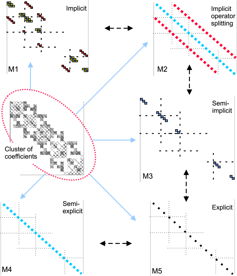
Figure 1: A schematic description of the hierarchical clustering of the coefficient matrix employed by the algorithm. Here, a cluster of coefficients is computed in the very early stage. The matrix-generator then selects the entries to be used for constructing the matrix coefficient appropriate for the solution procedure. Depending on the matrix used, the solution method may range from purely explicit to fully implicit. Interchange between solution methods is possible, as modifying, adding or removing entries is directly maintainable.

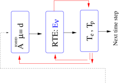
Figure 2: A schematic description of the hierarchical structure of the algorithm. Stage I corresponds to the implicit operator splitting approach (IOS), which is most appropriate for following the early time-dependent phases of the flow. The solutions obtained can then be used as initial conditions for Stage II, where the hydro-equations are solved as a single coupled system, followed by the magneto component, which is again solved as a single coupled system. Here, high spatial and temporal accuracies in combination with the prolongation/restriction strategy may be used. Similarly, the solutions obtained in this stage may be used as starting solutions for Stage III, where steady solutions for the fully coupled set of equations consisting of the zero moment of the radiation field and the MHD equations are sought. In this stage, pre–conditioned Krylov sub–space iterative methods are considered to be robust and efficient. The very last stage, Stage IV, corresponds to the case where solutions for the internal energy equations weakly coupled with the 5D radiative transfer equation are sought.

4 The hierarchical solution strategy - HSS

The set of hydrodynamical equations are solved within the context of the hierarchical solution strategy (HSS, see Hujeirat (2005)). HSS is based on constructing a coefficient matrix $A$, which results from linearizing the complete set of equations in a fully implicit manner. Noting that the conservative formulation of the HD-equations yields a matrix coefficient that is highly sparse, it is reasonable to design a procedure which selects the entries for constructing the approximate matrix $\hat{A}$ most appropriate for the flow problem. Depending on the structure of $\hat{A}$, a suitable iterative method within the context of defect-correction method may be employed to assure consistency and convergence.

For example, if we want to simulate a two-dimensional weakly compressible, non-magnetized and non-radiating flow between two concentric spheres, then the above-mentioned procedure is set to select the entries from the cluster of coefficients that corresponding just to the equations to be solved (see Fig. 1), which are used then to construct the preconditioning $\hat{A}$.

To clarify the procedure, we re-write the set of equations in a conservative vector form:

$$\frac{\partial\vec{q}}{\partial t}+L_{\mathrm{r,rr}}\vec{F}+L_{\mathrm{\theta,\theta\theta}}\vec{G}=\vec{f},$$ (27)

where $\vec{F}$ and $\vec{G}$ are fluxes of $q$, and $L_{\mathrm{r,rr}},\,L_{\mathrm{\theta,\theta\theta}}$ are first and second order operators that describe the advection and diffusion of the vector variables $\vec{q}$ in $\mathrm{r}$ and $\theta$ directions. $\vec{f}$ corresponds to the vector of source functions.

In order to enhance the mathematical consistency and increase the spatial and temporal accuracies of the numerical scheme without a substantial increase of the computational costs, we adopt the so-called prediction-correction iteration procedure. Therefore, we re-write Eq. (27) in residual form: $R=\frac{\partial\vec{q}}{\partial t}+L_{\mathrm{r,rr}}\vec{F}+L_{\mathrm{\theta,\theta\theta}}\vec{G}-\vec{f}=0$, and adopting a five star staggered grid discretization, we may apply the Newton-linearization to calculate the Jacobian, $J_{\mathrm{m1,n1}}\doteq\frac{\partial R_{\mathrm{m1}}}{\partial q_{\mathrm{n1}}}$, where $\mathrm{m1,n1}$ are integers that run over the number of equations and variables. The solution can be obtained then as follows:

$$\vec{q}^{i+1}=\vec{q}^{i}-J^{-1}_{\mathrm{m1,n1}}R^{i},$$

where $i$ is the iteration level. By inspection of the Jacobian J, it can be easily verified that it has the following block matrix structure:

$$\frac{{\delta q}_{\mathrm{j,k}}}{\delta t}+\underline{S}^{\mathrm{r}}{\delta q}_{\mathrm{j-1,k}}+{D}^{\mathrm{r}}{\delta q}_{\mathrm{j,k}}+\overline{S}^{\mathrm{r}}{\delta q}_{\mathrm{j+1,k}}$$

$$+\underline{S}^{\mathrm{\theta}}{\delta q}_{\mathrm{j,k-1}}+{D}^{\mathrm{\theta}}{\delta q}_{\mathrm{j,k}}+\overline{S}^{\mathrm{\theta}}{\delta q}_{\mathrm{j,k+1}}=RHS^{\mathrm{n}}_{\mathrm{j,k}},$$ (28)

where ${\delta q}=q^{i+1}-q^{i},$ and which, in the linear case, reduces to time-difference of $q$. The subscripts “j” and “k” denote the grid-numbering in the $\mathrm{r}$ and $\theta$ directions, respectively, and $RHS^{\mathrm{n}}=[\vec{f}-L_{\mathrm{r,rr}}\vec{F}-L_{\mathrm{\theta,\theta\theta}}\vec{G}]^{\mathrm{n}}$. $\underline{S}^{\mathrm{r,\theta}}$ and $\overline{S}^{\mathrm{r,\theta}}$ mark the sub-diagonal and super-diagonal block matrices, respectively. ${D}^{\mathrm{r,\theta}}$ corresponds to diagonal block matrices.
To outline the directional dependence of the block matrices, we re-write Eq. (27) in a more compact form:

$$\begin{array}[]{lll}&{\hskip 6.88889pt}\overline{S}^{\mathrm{\theta}}{\delta q}_{\mathrm{j,k+1}}&\\ +\underline{S}^{\mathrm{r}}{\delta q}_{\mathrm{j-1,k}}&+{D}_{\mathrm{mod}}{\delta q}_{\mathrm{j,k}}&+\overline{S}^{\mathrm{r}}{\delta q}_{\mathrm{j+1,k}}=RHS^{\mathrm{n}}_{\mathrm{j,k}}\\ &+\underline{S}^{\mathrm{\theta}}{\delta q}_{\mathrm{j,k-1}},&\end{array}$$ (29)

where ${D}_{\mathrm{mod}}=I/{\delta t}+{D}^{\mathrm{r}}+{D}^{\mathrm{\theta}}.$
This equation gives rise to at least four different types of solution procedures:

1. Classical explicit methods are very special cases in which the sub- and super-diagonal block matrices together with ${D}^{\mathrm{r}}$ and ${D}^{\mathrm{\theta}}$ are neglected. The only matrix to be retained here is $(1/{\delta t})\,\times\,$(the identity matrix), i.e., the first term on the LHS of Eq. (28). This yields the vector equation (see M5/Fig. 1):

   $$[\frac{I}{\delta t}]{\delta q}_{\mathrm{j,k}}=RHS^{\mathrm{n}}_{\mathrm{j,k}}.$$ (30)

2. Semi-explicit methods are obtained by preserving the diagonal entries, $d_{\mathrm{j,k}},$ of the block diagonal matrix ${D}_{\mathrm{mod}}$ (see M4/Fig. 1). This method has been verified to be numerically stable even when large Courant-Friedrichs-Levy (CFL) numbers are used. In particular, this method is absolutely stable if the flow is viscous-dominated.

3. Semi-implicit methods are recovered when neglecting the sub- and super-diagonal block matrices only, but retaining the block diagonal matrices (see M3/Fig. 1). In this case the matrix equation reads:

   $${D}_{\mathrm{mod}}{\delta q}_{\mathrm{j,k}}=RHS^{\mathrm{n}}_{\mathrm{j,k}}.$$ (31)

   We note that inverting ${D}_{\mathrm{mod}}$ is a straightforward procedure, which can be maintained analytically or numerically.

4. A fully implicit solution procedure requires retaining all the block matrices on the LHS of Eq. (28). This yields a global matrix that is highly sparse (M1/Fig. 1). In this case, semi-direct methods such as the “Approximate Factorization Method” (AFM: Beam, Warming, 1978) and the “Line Gauss-Seidel Relaxation Method” (-LGS: MacCormack, 1989) are considered to be efficient preconditioners for solving the set of radiative MHD-equations within the context of defect-correction iteration method (see Hujeirat (2005) and the references therein). Furthermore, Krylov sub-iterative methods may prove to be more efficient and robust than the above-mentioned semi-direct methods.

In the case that only stationary solutions are sought, convergence to steady state can be accelerated by adopting the so-called “Residual Smoothing Method” (Hujeirat, 2005) This method is based on associating a time step size with the local CFL-number at each grid point. While this strategy is efficient at providing quasi-stationary solutions within a reasonable number of iterations, it is incapable at providing physically meaningful time scales for features that possess quasi-stationary behaviour. Here we suggest to use the obtained quasi-stationary solutions as initial configuration and re-start the calculations using a uniform and physically relevant time step.

5 Numerical techniques

In this section we briefly describe several algorithmic steps for solving the continuity equation and the generalization procedure.

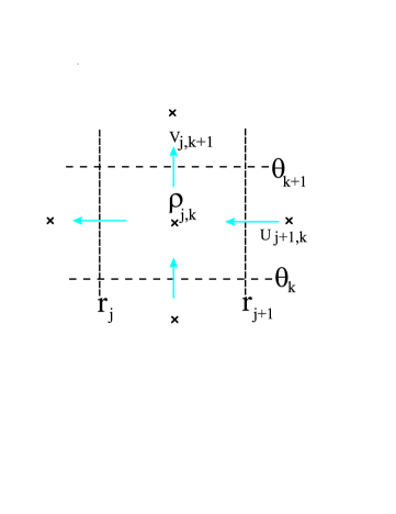
Figure 3: The location of the variables using the staggered grid discretization.

1. The continuity equation is discretized using the staggered grid strategy within the context of finite volume philosophy (Fig. 3).

   $$\frac{1}{\sqrt{-g}}\frac{\partial}{\partial r}\left.\left(\sqrt{-g/g_{rr}}DU\right)\right|_{\mathrm{j,k}}$$

   $$\Rightarrow\left.\frac{[\sqrt{{-g}/{g_{rr}}}\,U\overrightarrow{D^{r}}]^{r_{j+1}}_{r_{j}}}{[\int{\sqrt{-g}dr}]^{r_{j+1}}_{r_{j}}}\right|_{\mathrm{k}}=\left.\frac{[\sqrt{{-g}/{g_{rr}}}\,U\overrightarrow{D^{r}}]_{r=r_{j+1}}-[\sqrt{{-g}/{g_{rr}}}\,U\overrightarrow{D^{r}}]_{r=r_{j}}}{[\int{\sqrt{-g}dr}]^{r_{j+1}}_{r_{j}}}\right|_{\mathrm{k}},$$ (32)

   $$\frac{1}{\sqrt{-g}}\frac{\partial}{\partial\theta}\left.\left(\sqrt{-g/g_{\theta\theta}}\right)DV\right|_{\mathrm{j,k}}$$

   $$\Rightarrow\left.\frac{[\sqrt{-g/g_{\theta\theta}}V\overrightarrow{D^{\theta}}]^{\theta_{k+1}}_{\theta_{k}}}{[\int{\sqrt{-g/g_{\theta\theta}}d\theta}]^{\theta_{k+1}}_{\theta_{k}}}\right|_{\mathrm{j}}=\left.\frac{[\sqrt{-g/g_{\theta\theta}}V\overrightarrow{D^{\theta}}]_{\theta_{k+1}}-[\sqrt{-g/g_{\theta\theta}}V\overrightarrow{D^{\theta}}]_{\theta_{k}}}{[\int{\sqrt{-g}d\theta}]^{\theta_{k+1}}_{\theta_{k}}}\right|_{\mathrm{j}},$$ (33)

   where

   $$\overrightarrow{D^{r}}_{j,k}=\left\{\begin{array}[]{ll}D_{j,k}+f^{r}_{j,k}&\textrm{if}\,\,U_{j,k}<0\\ D_{j-1,k}+f^{r}_{j-1,k}&\textrm{if}\,\,U_{j,k}\geq 0\end{array}\right.\,;\,\overrightarrow{D^{\theta}}_{j,k}=\left\{\begin{array}[]{ll}D_{j,k}+f^{\theta}_{j,k}&\textrm{if}\,\,V_{j,k}<0\\ D_{j,k-1}+f^{\theta}_{j,k-1}&\textrm{if}\,\,V_{j,k}\geq 0\end{array}\right.$$ (34)

   The functions $f^{r}\textrm{ and }f^{\theta}$ are corrections for maintaining higher order spatial accuracies.

2. In order to obtain second order temporal accuracy, we write the continuity equation as follows:

   $$\frac{\delta D}{\delta t}+\vartheta L1^{n+1}(D)+(1-\vartheta)L1^{n}(D)=0,$$ (35)

   where $\vartheta$ denotes the parameter of the stabilized Crank-Nicolson method for achieving second order temporal accuracy. $L1_{h}$ resembles the advection operator at the new time level (n+1) and the old time level (n) and $\delta D=D^{n+1}-D^{n}.$ Taylor-expanding the variable $D^{n+1}$ in time and considering first order terms only, the continuity equation gets the following form:

   $$\frac{\delta D}{\delta t}+\vartheta L1^{n+1}(\delta D)+L1^{n}(D)=0,$$ (36)

3. Define the defect $d_{\mathrm{j,k}}$ at every grid point:

   $$d_{\mathrm{j,k}}=-\frac{\delta D}{\delta t}-\vartheta L1^{n+1}_{\mathrm{high}}(D)-(1-\vartheta)L1^{n}_{\mathrm{high}}(D)|_{j,k},$$ (37)

   where the subscript ”high” means that the transport operators are evaluated using a spatially accurate advection scheme.
   

4. Define at each grid point the following operator:

   $$LD=-\frac{\delta D}{\delta t}-\vartheta L1^{n+1}_{\mathrm{low}}(D)-(1-\vartheta)L1^{n}_{\mathrm{high}}(D)|_{j,k}.$$ (38)

   Compute the following entries at each grid point:

   $$\underline{S}^{r}_{j,k}=\frac{\partial LD}{\partial D_{j-1,k}},\,\,\mathcal{D}_{j,k}=\frac{\partial LD}{\partial D_{j,k}},\,\,\overline{S}^{r}_{j,k}=\frac{\partial LD}{\partial D_{j+1,k}},$$

   $$\underline{S}^{z}_{j,k}=\frac{\partial LD}{\partial D_{j,k-1}},\,\,\overline{S}^{z}_{j,k}=\frac{\partial LD}{\partial D_{j,k+1}}$$ (39)

5. In the one-dimensional case, the following matrix equation should be solved at each grid point:

   $$\left(\begin{array}[]{ccc}\underline{S}_{j,k},&\mathcal{D}_{j,k},&\overline{S}_{j,k}\end{array}\right)\left(\begin{array}[]{l}\delta D_{j-1,k}\\ \delta D_{j,k}\\ \delta D_{j+1,k}\\ \end{array}\right)=\left(\begin{array}[]{l}d_{j-1,k}\\ d_{j,k}\\ d_{j+1,k}\\ \end{array}\right),\textrm{ where j=1, J, and k= const.}$$ (40)

   For J number of grid points in the radial direction, this yields the tri-diagonal matrix equation:

   $$\left(\begin{array}[]{ccccc}{\mathcal{D}_{1}}&{{\overline{S}}_{1}}&&&\\ {{\underline{S}}_{2}}&{\mathcal{D}_{2}}&{{\overline{S}}_{2}}&&\\ &\ddots&\ddots&\ddots&\\ &&{{\underline{S}}_{J}}&{\mathcal{D}_{J}}&\\ \end{array}\right)\left(\begin{array}[]{c}{\delta D_{1}}\\ {\delta D_{2}}\\ \vdots\\ {\delta D_{N}}\\ \end{array}\right)=\left(\begin{array}[]{c}{d_{1}}\\ {d_{2}}\\ \vdots\\ {d_{N}}\\ \end{array}\right)~{}~{}~{}~{}\textrm{ for constant k}$$ (41)

   Although this matrix equation is linear in D, it should be solved iteratively to recover the high spatial accuracy on the right hand side.
   

   Similarly, if the continuity and the radial momentum equation are to be solved in one dimension as a coupled system, we may obtain the following relation at each grid point:

   $$\left(\begin{array}[]{|cc|cc|cc|}{L11_{j-1}}&{L12_{j-1}}&{L11_{j}}&{L12_{j}}&{L11_{j+1}}&{L12_{j+1}}\\ {L21_{j-1}}&{L22_{j-1}}&{L21_{j}}&{L22_{j}}&{L21_{j+1}}&{L22_{j+1}}\\ \end{array}\right)\left(\begin{array}[]{l}\left\{\begin{array}[]{l}{\delta D}\\ {\delta M}\\ \end{array}\right\}_{\mathrm{j-1}}\\ \left\{\begin{array}[]{l}{\delta D}\\ {\delta M}\\ \end{array}\right\}_{\mathrm{j}}\\ \left\{\begin{array}[]{l}{\delta D}\\ {\delta M}\\ \end{array}\right\}_{\mathrm{j+1}}\end{array}\right)=\left(\begin{array}[]{l}\left\{\begin{array}[]{l}{d^{\mathrm{D}}}\\ {d^{\mathrm{M}}}\\ \end{array}\right\}_{\mathrm{j-1}}\\ \left\{\begin{array}[]{l}{d^{\mathrm{D}}}\\ {d^{\mathrm{M}}}\\ \end{array}\right\}_{\mathrm{j}}\\ \left\{\begin{array}[]{l}{d^{\mathrm{D}}}\\ {d^{\mathrm{M}}}\\ \end{array}\right\}_{\mathrm{j+1}}\end{array}\right)$$ (42)

      for j = 1, J and k = const.,

   where $Lmn_{l}=\frac{\partial Lm}{\partial q_{n}}|_{j=l}.$ Specifically, L1 is the density equation and L2 the momentum equation.
   For J number of points this yields a tri-diagonal block matrix, in which each block has the dimension $2\times 2.$
   For a given set of equations in one dimension, we have just to replace the above $2\times 2$ block matrix by a square block matrix whose dimensions are $N_{\mathrm{eq}}\times N_{\mathrm{eq}}$, where $N_{\mathrm{eq}}$ is the number of unknown variables:

   $$\left(\begin{array}[]{cccc}{{\square}}&{{\square}}&&\\ {{\square}}&{{\square}}&{{\square}}&\\ &\ddots&\ddots&\ddots\\ &&{{\square}}&{{\square}}\\ \end{array}\right)\left(\begin{array}[]{l}{\delta\overline{q}_{1}}\\ {\delta\overline{q}_{2}}\\ \vdots\\ {\delta\overline{q}_{J}}\\ \end{array}\right)=\left(\begin{array}[]{c}{\overline{d}_{1}}\\ {\overline{d}_{2}}\\ \vdots\\ {\overline{d}_{J}}\\ \end{array}\right).$$ (43)

   $\overline{q}$ here is a vector of $N_{\mathrm{eq}}$ entries.
   

   The extension into two-dimensions gives rise to a matrix equation of the following form:

   $$\tilde{A}\left(\begin{array}[]{l}{\delta\overline{q}_{1,1}}\\ \vdots\\ {\delta\overline{q}_{J,1}}\\ {\delta\overline{q}_{1,2}}\\ \vdots\\ {\delta\overline{q}_{J,K}}\\ \end{array}\right)=\left(\begin{array}[]{l}{\overline{d}_{1,1}}\\ \vdots\\ {\overline{d}_{J,1}}\\ {\overline{d}_{1,2}}\\ \vdots\\ {\overline{d}_{J,K}}.\\ \end{array}\right)$$ (44)

   The matrix $\tilde{A}$ has a similar structure as M1 in Fig. 1. This matrix equation is solved iteratively, using a non-direct inversion procedure.

6 Test calculations

The verification tests of the Newtonian version of the present algorithm have been presented in a series of papers (see Hujeirat (2005) and the references therein). Nevertheless the modifications made here are serious and deserve appropriate test calculations to ensure bug-free runs as well as a consistent re-production of the results in the Newtonian regime.
In the following we briefly mention several of the test calculations performed:

• The shock tube problem - STP
  In the case of low fluid-velocities, the modification made should enable capturing of shocks propagating at sub-relativistic speeds, irrespective of the accuracies used. Therefore, we have applied the algorithm to the well-known Sod-problem (see Hujeirat (1995) and the references therein). Fig. 4 shows that the algorithm is indeed capable of re-producing Sod’s solution with high accuracy.

• The ultra-relativistic shock tube problem
  The speed of the shocks in the Sod’s problem can be made arbitrary large, depending on the initial ratio of the pressure in the tube. While non-relativistic solvers may produce propagating velocities that exceeds the speed of light, a conservative and accurate relativistic solver should produce velocities that can be extremely close to but never exceed the speed of light.
  In Fig. 5 the one-dimensional profiles of the density, velocity, temperature and Lorentz factor $u^{\mathrm{t}}$ are displayed. These profiles agree qualitatively with the analytical solution of the relativistic STP provided by Marti and Müller (2003). In a forthcoming paper, we intend to quantitatively compare the profiles for extremely large Lorentz factors.

  Fig. 5 demonstrates the strong robustness of the algorithm and its capability to capture the propagation of extreme ultra-relativistic shocks in which the Lorentz factor is of order 1000. Such robustness is essential to enable modeling jetted Gamma-Ray bursts, where the Lorentz factors are in the excess of several hundreds.

  

  Figure 4: The classical non-relativistic shock tube problem. The profiles of the density, velocity, temperature and pressure are displayed. The advection scheme used here is second order in time and third order in space. 200 uniformly distributed finite volume cells are used.

  

  Figure 5: The ultra-relativistic shock tube problem. The radial distributions of the density, radial velocity, temperature and the modified Lorentz factor $U^{t}$ are shown. The accuracy of the scheme and the number of points are identical to those in Fig. 4. This calculation shows that shocks propagating with Lorentz factors of order 1000 can be safely treated with our algorithm.

• Relativistic Bondi accretion onto Schwarzschild black holes
  This problem is appropriate for testing the capability of the solver at treating transonic stationary accretion flows onto Schwarzschild black holes, assuming perfect spherical symmetry. This problem has been investigated by several authors (see Michel (1972), also see Hawley et al. (1984a, b) for a comprehensive description of the numerical treatment). In this problem, a constant flux of an ideal gas is said to be accreted by a non-rotating black hole. Depending on location of the outer boundary and on the temperature of the flow, the initially subsonic inflow should make a transition into the super-sonic regime at a specific radius, which appears to be determined entirely by the constant of motion. On the other hand, the Lorentz factor of the flow as it crosses the inner boundary should approach the speed of light, depending on how close the inner radius is to the event horizon. In Fig. 6 we display the radial distributions of the velocity, density, temperature, Lorentz factor and the Mach number, which clearly well-agree with the known analytical solutions. In obtaining these results we used a pseudo time-stepping scheme to enhance convergence. The very last time step size in this calculations corresponds to Courant number 2000, approximately.

  

  Figure 6: The Bondi accretion problem onto a Schwarzschild black hole. The profiles of the radial velocity, the relativistic density, temperature, the Lorentz factor $U^{t}$ and the radial Mach number. In the lower-right panel profiles of the Courant number (solid line) and the corresponding residual (dashed line) versus the iteration number are displayed. Although the problem is spherically symmetric, the calculations have been carried out using 200 grid points in the radial and 30 in the horizontal-direction. The accuracy of the advection scheme is set to be first order in time and third order in space. This test enables us to examine the capability of the algorithm at capturing steady solutions that are essentially one-dimensional using a 2D numerical scheme. We have verified that the 30-profiles in the radial direction obtained at different $\theta$ are identical to machine- accuracy.

• Standing shocks around black holes
  The purpose of this test is mainly to examine the capability of the algorithm at re-producing the formation of the two-dimensional curved standing shocks around a Schwarzschild black hole that have been obtained using the Newtonian version of the algorithm.

  This problem is similar to the forward facing step in computational fluid dynamics. Here a cold and dense disk has been placed in the innermost equatorial region: $[1\leq r\leq 10]\times[-0.3\leq\theta\leq 0.3]$ (see Figures 7 and 8). Vanishing in- and out-flow conditions have been imposed at the boundaries of the cold disk. The gas surrounding the disk is taken to be inviscid, thin, hot and non-rotating. The cold disk here serves as a two-dimensional barrier that disturbs the gas from otherwise a spherically symmetric freely falling flow onto a Schwarzschild black hole and, instead, it forces the inflow to form a curved shock which eclipses the cold disk.

  In solving the HD-equations, an advection scheme of third order spatial accuracy and of first order accuracy in time has been used.

  Hence the scheme is taken to be highly diffusive in time in order to damp oscillations and to accelerate convergence into steady-state. The domain of calculation is sub-divided into 200 strongly-stretched finite volume cells in the radial and 60 in the horizontal direction. In Fig. 8 the 1D radial and horizontal profiles, the 2D configuration of the density, temperature and the velocity field are shown. Indeed, the algorithm shows that it is numerically stable and capable of capturing steady-state shocks with complicated shock structures even for large CFL-numbers.

  

  

  

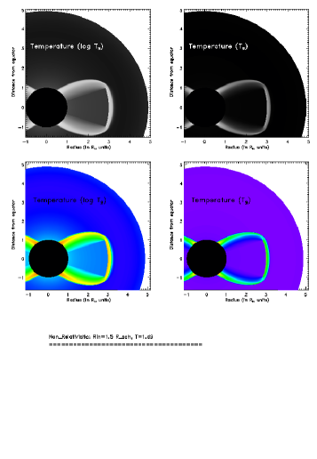
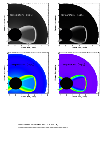
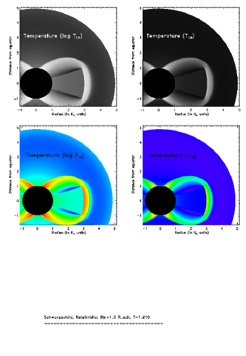
  Figure 7: The 2D distribution of the temperature (in units of $10^{9}$K) of a freely falling non-relativistic gas onto a Schwarzschild black hole surrounded by a static cold disk (top panel). In this figure, color gradients run as follows: red color corresponds to large temperature-values, green to intermediate and blue to low values. The distribution in the second and third panels have been obtained using the general relativistic version of the algorithm. Here the inflowing matter across the outer boundary has the temperatures $10^{9}$K (middle) and $10^{10}$K (bottom).

  

  

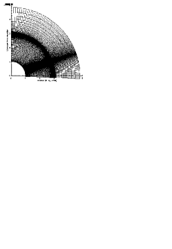
  Figure 8: Distribution of the grid points used in the calculations. A strong non-uniform distribution of the grid points has been constructed to enable accurate capturing of standing shocks surrounding the cold disk. The tensor-product mesh consists of 275 finite volume cells in the radial and 130 in the horizontal direction, respectively. In the lower panel the profiles of the density, temperature, radial and vertical velocities along the equator and horizontal along the constant radius $r=2.5$ are shown.

7 Summary

In this paper we have extended the previous Newtonian implicit algorithm to enable solving the hydrodynamical equations in general relativity. The 3D axi-symmetric hydrodynamical equations have been presented in the background of a Kerr metric of a black hole using the Boyer-Lindquist coordinates. The equations have been formulated in conservative form and subsequently solved numerically, using the finite volume formulation. The new extension can be well accommodated within the hierarchical solution scenario, in which the degree of implicitness can be made dynamical, depending on the hydrodynamical problem in hand. In particular, for modeling strongly time-dependent astrophysical flows, such as moving shocks, the pre-conditioners used are tri-diagonal matrices that are solved successively. Although the computational costs per time step may be one order of magnitude larger than their explicit counterparts, this can be compensated through a reduction of the overall number of time steps required to recover a physically reliable time scale.

On the other hand, the efficiency and robustness of the HSS are superior, if the solutions sought are stationary or quasi-stationary, irrespective of whether the flow is dissipative or not.

Finally, a unification scheme for various numerical methods has been presented. In particular, the HSS algorithm enables the construction of a large variety of solvers, in which the degree of implicitness may range from purely explicit up to strongly implicit, depending on the physical properties of the underlying flow problem. Thus, the HSS is actually a unified algorithm for treating weakly compressible, incompressible, time-dependent, time-independent, radiative, magnetized non-dissipative or strongly dissipative flows. As a consequence, using the HSS algorithm, we are able to save a large number of working hours which otherwise would go in designing different solvers for different physical problems.
In a subsequent paper, we intend to discuss and describe the inclusion of the magnetohydrodynamical equations in general relativity into the present solver.

Acknowledgment A.H. thanks Prof. J. Dušek for reading the manuscript and for the hospitality during his visit to the Institut de mechanique des fluides et des solides, CNRS and the Louis Pasteur University in Strasbourg. This work has been partially supported by the Klaus-Tschira Stiftung under the project number 00.099.2006.

References

- Alay et al. (1999) Aloy, M.-A., Ibanez, J.M., Mart, J.M., Müller, E., 1999, ApJS, 122, 151 (GENESIS)
- Anninos, Fragile (2003) Anninos, P., Fragile, P. C., 2003, ApJ. Suppl. Ser., 144, Iss. 2, 243-257
- Anninos et al. (2005) Anninos, P., Fragile, P. C., Salmonson, J.D., 2005, ApJ, 635, 723
- Baiotti et al. (2003) Baiotti, L., Hawke, I., Montero, P.J., Rezzolla, L., 2003, MSAIS, 1, 210
- Banyuls et al. (1997) Banyuls, F., Font, J. A.,Ibáñez, J. M., Martí, J. M., Miralles, J. A., 1997, ApJ, 476, 221
- Beam, Warming (1978) Beam, R.M., Warming, R.F., 1978, AIAA, 16, 393
- Bodenheimer et al. (1978) Bodenheimer, P., Tohline, J. E., Black, D. C., 1978, BAAS, 10, 655
- Böhmer, Stetter (1984) Böhmer, K., Stetter H. J., 1984, “Defect Correction Methods: Theory and Applications”, Springer–Verlag, Wien-New York
- Clarke (1996) Clarke, D.A., 1996, APJ, 457, 291
- Del Zanna, Bucciantini (2002) Del Zanna, L., Bucciantini, N., 2002, A&A, 390, 1177-1186
- Del Zanna et al. (2007) Del Zanna, L., Zanotti, O., et al., 2007, A&A, 473, 11
- De Villiers, Hawley (2003) De Villiers, J.-P., Hawley, J.F., 2003, ApJ, 589, 458
- Enander (1997) Enander, R., 1997, SIAM J. Sc. Comp., 18, 5, 1243
- Eulderink, Mellema (1995) Eulderink, F., Mellema, G., 1995, Astron. Astophys. Suppl. Ser., 110, 587
- Falle (2003) Falle, S.A.E.G., 2003, astro-ph/0308396
- Fletcher (1988) Fletcher, C.A.J., 1988, ”Computational Techniques for Fluid Dynamics”, Vol. I, II, Springer-Verlag, London
- Font et al. (2000) Font, J.A., Miller, M., Suen, W., Tobias, M., 2000, Phys. Rev. D, 61, 044011
- Font (2003) Font, J.A., 2003, LRR, 6, 4
- Fryxell et al. (2000) Fryxell, B. et al., 2000, ApJS, 131, 273-334 (FLASH)
- Gammie et al. (2003) Gammie, C. F., McKinney, J. C., Tóth, G., 2003, ApJ, 589, 444-457 (HARM)
- Gardiner, Stone (2006) Gardiner, T.A., Stone, J.M., 2006, ASPC, 359, 143
- Hackbusch (1994) Hackbusch, W., 1994, “Iterative Solution of Large Sparse Systems of Equations”, Springer–Verlag, New York-Berlin-Heidelberg
- Hirsch (1988) Hirsch, C., 1988, ”Numerical Computation of Internal and External Flows”, Vol. I, II, John Wiley & Sons, New York
- Hujeirat (1995) Hujeirat, A., 1995, A&A,295, 268
- Hujeirat, Rannacher (2001) Hujeirat, A., Rannacher, R., 2001, New Ast. Reviews, 45, 425
- Hujeirat (2005) Hujeirat, A., 2005, CoPhC, 168, 1
- Hawley et al. (1984a) Hawley, J. F., Smarr, L. L., Wilson, J. R., 1984a, ApJ, 277, 296-311
- Hawley et al. (1984b) Hawley, J. F., Smarr, L. L., Wilson, J. R., 1984b, ApJS, 55, 211-246
- Koide et al. (1999) Koide, S., Shibata K., Kudoh, T., 1999, ApJ, 522, 727
- Komissarov (2004) Komissarov, S.S., 2004, MNRAS, 350, 1431
- Liebendörfer et al. (2002) Liebendörfer, M., Rosswog, S., Thielemann, F.-K., 2002, ApJS, 141, 229L
- MacCormack (1989) MacCormack, R., 1989, Computers and Fluids, 17, 135
- Marti and Müller (2003) Marti, J.M., Müller, E., 2003, LRR, 6, 7
- Michel (1972) Michel, F.C., 1972, Ap&SS, 15, 163
- Mignone, Bodo (2003) Mignone, A., Bodo, G., 2003, NewAR, 47, 581
- Mignone et al. (2007) Mignone, A., Bodo, G., Massaglia, S., Matsakos, T., Tesileanu, O., Zanni, C., Ferrari, A., 2007, ApJS, 170, 228-242 (PLUTO)
- Meliani et al. (2007) Meliani, Z., Keppens, R., et al., 2007, MNRAS, 376, 1189
- Mizuno et al. (2006) Mizuno, Y., Nishikawa, J.-I., et al., 2006, astro-ph/0609004 (RAISHIN)
- Nagel et al. (2006) Nagel, W.E., Jäger, W., Resch, M. (Eds.), 2006, ”High Performance Computing in Science and Engineering ’06”, Springer, Berlin, Heidelberg, New York, 2006
- O’Shea et al. (2004) O’Shea, B.W., Bryan, G., Bordner, J., Norman, M. L., Abel, T., Harkness, R., Kritsuk, A., 2004, astro-ph/0403044 (ENZO)
- Richtmyer, Morton (1967) Richtmyer, R.D., Morton, K.W., 1967, ”Difference methods for initial value problems”, 2nd ed., Interscience, New York
- Shibata, Sekiguchi (2005) Shibata, M., Sekiguchi, Y., 2005, PhRvD, 72, 4, 044014
- Spindeldreher (2002) Spindeldreher, S., PhD thesis, 2002, Ruperto-Carola University of Heidelberg, Germany
- Stetter (1978) Stetter, H.J., 1978, Numer. Math., 29, 425–443
- Stone, Norman (1992) Stone, J.M., Norman, M.L., 1992, ApJS, 80, 753
- Swanson, Turkel (1997) Swanson, R.C., Turkel, E., 1997, NASA,TP-3631, 81
- Swesty (1995) Swesty, F.D., 1995, ApJ, 445, 811
- Tassoul (1978) Tassoul, J.-L., “Theory of rotating stars”, PUP, Priceton
- Tóth et al. (1998) Tóth, G., Keppens, R., Botchev M.A., 1998, A&A, 332, 1159 (VAC)
- Wang et al. (2007) Wang, P., Abel, T., Zhang, W., 2007, astro-ph/0703742 (ENZO)
- Wilson (1972) Wilson, J. R., 1972, ApJ, 173,431
- Wuchterl (1990) Wuchterl, G., 1990, A&A, 238, 83
- Zhang, MacFadyen (2006) Zhang, W., MacFadyen, A. I., 2006, ApJS, 164, 255-279 (RAM)
- Ziegler (1998) Ziegler, U., 1998, Comp. Phys. Comm., 109, 111 (NIRVANA)