Long-time electron spin storage via dynamical suppression of
hyperfine-induced decoherence in a quantum dot

Abstract

The coherence time of an electron spin decohered by the nuclear spin environment in a quantum dot can be substantially increased by subjecting the electron to suitable dynamical decoupling sequences. We analyze the performance of high-level decoupling protocols by using a combination of analytical and exact numerical methods, and by paying special attention to the regimes of large inter-pulse delays and long-time dynamics, which are outside the reach of standard average Hamiltonian theory descriptions. We demonstrate that dynamical decoupling can remain efficient far beyond its formal domain of applicability, and find that a protocol exploiting concatenated design provides best performance for this system in the relevant parameter range. In situations where the initial electron state is known, protocols able to completely freeze decoherence at long times are constructed and characterized. The impact of system and control non-idealities is also assessed, including the effect of intra-bath dipolar interaction, magnetic field bias and bath polarization, as well as systematic pulse imperfections. While small bias field and small bath polarization degrade the decoupling fidelity, enhanced performance and temporal modulation result from strong applied fields and high polarizations. Overall, we find that if the relative errors of the control parameters do not exceed 5$\%$, decoupling protocols can still prolong the coherence time by up to two orders of magnitude.

I Introduction

Electron and nuclear spin degrees of freedom are promising candidates for a variety of quantum information processing (QIP) devices DiVincenzo (1995); AwschalomSciAm02 ; Baugh07 . While the wide range of existing microfabrication techniques make solid-state architectures extremely appealing in terms of large-scale integration, such an advantage is seriously hampered by the noisy environments which are typical of solid-state systems, and are responsible for unwanted rapid decoherence. For an electron spin localized in a GaAs quantum dot (QD) Loss and DiVincenzo (1998), for instance, the relevant coherence time is extremely short: at typical experimental temperatures (T $\sim 100$ mK) and sub-Tesla magnetic fields, the electron free induction decay (FID) time $T_{2}^{*}\sim 10$ ns Petta et al. (2005); Johnson et al. (2005); Koppens et al. (2005), the dominant decoherence mechanism being the hyperfine coupling to the surrounding bath of Ga and As nuclear spins. Although efforts for achieving faster gating times may contribute to alleviate the problem, it remains both highly desirable and presently more practical to extend the coherence time of the central system (the electron spin) in the presence of the spin bath.

Several proposals have been recently put forward to meet this challenge. A first strategy is to manipulate the spin bath. Polarizing the nuclear spins, for instance, may significantly increase the coherence time Burkard et al. (1999); Deng and Hu (2006), provided that nuclear-spin polarization $\gtrsim 99\%$ may be achieved. This, however, remains well beyond the current experimental capabilities. Another suggestive possibility, based on narrowing the distribution of nuclear spin states Coish04 ; Stepanenko et al. (2006); Klauser06 , has been predicted to enhance electron coherence by up to a factor of hundred, upon repeatedly measuring and pumping the electron into an auxiliary excited trion state – which also appears very challenging at present.

As an alternative approach, direct manipulation of the central spin by means of electron spin resonance (ESR) Gerstein and Dybowski (1985) and dynamical decoupling (DD) Haeberlen (1976); Slichter (1992); Viola and Lloyd (1998); Viola et al. (1999) techniques appears ideally suited to hyperfine-induced decoherence suppression, in view of the long correlation time and non-Markovian behavior which distinguish the nuclear spin reservoir. A single-pulse Hahn-echo protocol has been implemented recently in a double-QD device Petta et al. (2005), increasing the coherence time by two orders of magnitude. Significant potential of more elaborated pulse sequences, such as the multi-pulse Carr-Purcell-Meiboom-Gill (CPMG) protocol Witzel and Sarma (2007) and concatenated DD (CDD) Khodjasteh and Lidar (2005, ); Bergli and Glazman ; Yao et al. (2007), has been established theoretically for a single QD subjected to a strong external bias field, whereby the electron effectively undergoes a purely dephasing process. The DD problem for the more complex situation of a zero or low bias fields, where pure dephasing and relaxation compete, has been recently examined in Refs. Zhang et al., 2007a, . Having established the existence of highly effective DD schemes for electron spin storage, the purpose of this work is twofold: first, to gain a deeper understanding of the factors influencing DD performance and the range of applicability of conclusions based on analytical average Hamiltonian theory (AHT) approaches; and second, to assess the influence of various factors which may cause the system and/or control Hamiltonians to differ from the idealized starting point chosen for analysis.

Aside from its prospective practical significance, developing and benchmarking strategies for decoherence suppression in various spin nanosystems is interesting from the broader perspective of quantum control theory. In particular, standard theoretical tools usually employed for the analysis of DD performance, such as AHT and the Magnus Expansion (ME), have very restrictive formal requirements of applicability (very fast control time scales, bounded environments, etc), which may be hard to meet in realistic systems. Thus, in-depth studies of physically motivated examples are essential to understand how to go beyond the formal error bounds sufficient for convergence, and to identify more realistic necessary criteria for DD efficiency. In this sense, a QD system, described by the central spin model (a central spin-$1/2$ interacting with a bath of $N$ external spins Gaudin (1976); Prokof’ev and Stamp (2000)) both provides a natural testbed for detailed DD analysis, and paves the way to understanding more complex many-spin central systems.

In this work, we present a quantitative investigation of DD as a strategy for robust long-time electron spin storage in a QD. The content of the paper is organized as follows. In Sec. II, we lay out the relevant control setting, by describing the underlying QD model as well as the deterministic and randomized DD protocols under consideration. Among periodic schemes, special emphasis is devoted to the concatenated protocol (PCDD₂), which was identified as the best performer for this system in Ref. Zhang et al., 2007a. Exact AHT results are obtained up to second-order corrections in the cycle time, which allow additional physical insight on the underlying averaging and on DD-induced bath renormalization to be gained. Details on the methodologies followed to assess the quality of DD and to effect exact numerical simulations of the central spin coupled to up to $N=25$ bath spins are also included in Sec. II.

In Sec. III, numerical results on best- and worst-case performance of DD protocols for short evolution times are presented and compared with analytical predictions from AHT/ME under convergence conditions – in particular, $\omega_{c}\tau\ll 1$, where $\omega_{c}$ and $\tau$ are the upper cutoff frequency of the total system-plus-bath spectrum, and the time interval between (nearly instantaneous) consecutive control operations, respectively. Evolution times as long as $\sim 1000T_{2}^{*}$ for $\tau\lesssim T_{2}^{*}$ are able to be investigated numerically, other decoherence mechanisms becoming relevant for yet longer times. In the best-case scenario, where decoherence of a known initial state may be frozen under appropriate cyclic DD protocols Zhang et al. (2007a), the dependence of the attainable asymptotic coherence value on $\tau$ is elucidated in the small $\tau$ region. Sec. IV is devoted to further investigating the effect of experimentally relevant system features and/or non-idealities, such as the presence of residual dipolar couplings between the nuclear spins, the influence of an applied bias magnetic field, and the role of initial bath polarization. In Sec. V, the effect of systematic control imperfections such as finite width of pulses and rotation angle errors is quantitatively assessed. We present conclusions in Sec. VI.

II System and control assumptions

In this section we describe the model spin-Hamiltonian for a typical semiconductor QD, and typical picture of the decoherence dynamics of an electron spin in a QD. We present the DD methods used to suppress the electron spin decoherence and the metrics for DD performance, followed by numerical methods we employed.

II.1 QD model Hamiltonian

The decoherence dynamics of an electron spin $\bf S$ localized in a QD and coupled to a mesoscopic bath consisting of $N$ nuclear spins ${\bf I}_{k}$, $k=1,\dots N$, may be accurately described by the effective spin Hamiltonian Dobrovitski and De Raedt (2003); Al-Hassanieh et al. (2006); Zhang et al. (2006); Taylor et al. ; Zhang et al. (2007a, )

$$H=H_{S}+H_{B}+H_{SB},$$ (1)

where, in units $\hbar=1$,

$$H_{S} = \omega_{0}S_{z},$$ (2)

$$H_{B} = \sum_{k=1}^{N}\sum_{\ell<k=1}^{N}\Gamma_{k\ell}({\bf I}_{k}\cdot{\bf I}_{\ell}-3I^{z}_{k}I^{z}_{\ell}),$$ (3)

$$H_{SB} = \sum_{k=1}^{N}A_{k}{\bf S}\cdot{\bf I}_{k},$$ (4)

Here, the Hamiltonian $H_{S}$ describes the electron spin, $\omega_{0}=g_{e}^{*}\mu_{B}B_{0}$ being the Zeeman splitting in an external magnetic field $B_{0}$, $g_{e}^{*}$ is the effective Landé factor of the electron spin, and $\mu_{B}$ is the Bohr’s magneton. The Hamiltonian $H_{B}$ is the bath Hamiltonian, describing dipolar interactions with strength $\Gamma_{k\ell}$ between nuclear spin $k$ and $\ell$. For our analysis, a nearest-neighbor approximation to $H_{B}$ is adequate, with $\Gamma_{k\ell}$ taken as random numbers uniformly distributed between $[-\Gamma_{0},\Gamma_{0}]$, so that the parameter $\Gamma_{0}$ upper-bounds the strength of intra-bath couplings. The relevant system-bath coupling Hamiltonian $H_{SB}$ accounts for the Fermi contact hyperfine interaction, the coupling parameter $A_{k}=(8\pi/3)g_{e}^{*}\mu_{B}g_{n}\mu_{n}u^{2}({\mathbf{x}}_{k})$ being determined by the electron density $u^{2}({\mathbf{x}}_{k})$ at the $k$-th nuclear spin site ${\mathbf{x}}_{k}$ and by the Landé factor of the nuclei $g_{n}$. Other small contributions to the total QD Hamiltonian, such as the Zeeman splitting of the nuclear spins and anisotropic electron-nuclear couplings, may be neglected for the current purposes Zhang et al. (2006); Taylor et al. (see, however, Ref. Hodges07, for recent developments on controllability in the presence of anisotropic hyperfine couplings).

Upon tracing over the nuclear-spin reservoir, the electron spin described by Eq. (1) undergoes fast decoherence with a characteristic FID time of

$$T_{2}^{*}\simeq\frac{1}{A}\sqrt{\frac{8}{N}\frac{3}{4I(I+1)}},\;\;\;\;A=\sqrt{\frac{\sum_{k}A_{k}^{2}}{N}},$$

where $A\approx 10^{-4}\mu$eV for typical GaAs QDs with $N=10^{6}$ $I_{k}=I=3/2$ nuclear spins Paget et al. (1977); Zhang et al. (2006). This results in a $T_{2}^{*}$ value of about $10$ ns Johnson et al. (2005); Koppens et al. (2005); Petta et al. (2005); Taylor et al. , which is too short for QIP applications. In simulations, we shall neglect the $I$-dependence of the FID time and simply set the nuclear spin value to $I_{k}=1/2$ for all $k$. The FID time also turns out to depend very weakly on the applied bias field $B_{0}$ as long as $B_{0}$ is smaller than or comparable to the Overhauser field of the unpolarized nuclear spins Zhang et al. (2006). A similar conclusion holds for a weakly polarized nuclear spin bath, with polarization $p\ll 1$. Throughout this paper, energies shall be expressed in units of $A$, and time shall be expressed in units of $1/A$. Since $\Gamma_{0}\ll A_{k}$ for typical GaAs QDs Taylor et al. , we shall take $\Gamma_{0}=0$ (hence $H_{B}=0$) unless explicitly stated.

II.2 QD decoupling protocols

Compared to other decoherence control strategies, DD has many attractive features: it is a purely open-loop control method which, as such, avoids the need of measurements and/or feedback; it does not rely on a particular initial state which might be hard to prepare; its design and implementation may significantly benefit from the extensive expertise available from nuclear magnetic resonance (NMR) and ESR techniques.

We shall first assume to have access to ideal control resources, and defer the discussion of control limitations to Sec. V. In this idealized setting, DD of the electron spin is implemented by subjecting it to a sequence of bang-bang $\pi_{\hat{\bm{n}}}$ pulses Viola and Lloyd (1998), each instantaneously rotating the spin ${\mathbf{S}}$ along a given control axis $\hat{\bm{n}}$ by an angle $\pi$. Consecutive pulses are separated by a time interval $\tau$, resulting in a total time-dependent Hamiltonian of the form

$$H_{tot}(t) = H_{c}(t)+H,$$

$$H_{c}(t) = \sum_{\ell}\pi({\bf S}\cdot{\hat{\bm{n}}_{\ell}})\delta(t-\ell\tau),$$ (5)

where $\delta(\cdot)$ is the delta function, $\ell=1,2,\dots$ labels the applied pulses, and $H$ is given by Eq. (1). The evolution of the coupled electron-nuclear system in the physical frame is then described by the unitary propagator

$$U(t) = {\mathcal{T}}\exp\left[-i\int_{0}^{t}H_{tot}(s)ds\right],$$ (6)

where $\mathcal{T}$ denotes as usual temporal ordering.

II.2.1 Deterministic single-axis DD

DD protocols involving control rotations of the central spin about a fixed axis achieve selective averaging of spin components perpendicular to the rotation axis. Such sequences are effective when a preferred direction is present either in the underlying physical Hamiltonian or in the initial quantum state to preserve. For instance, in the presence of a strong static bias field, $B_{0}\gtrsim 1$ T, electron spin flips are energetically suppressed, and pure dephasing in the transverse direction is the dominant decoherence source Shenvi et al. (2005); de Sousa et al. (2005); Khodjasteh and Lidar ; Witzel and Sarma (2007). In such a situation, the interaction Hamiltonian Eq. (4) simplifies to

$$H_{\rm eff}=S_{z}\sum_{k}A^{\prime}_{k}I_{k}^{z},$$ (7)

with renormalized coupling constants $A^{\prime}_{k}$. The $z$-component of the central spin remains constant, while the transverse component $s_{\perp}=\sqrt{\langle S_{x}\rangle^{2}+\langle S_{y}\rangle^{2}}$ undergoes Gaussian FID with time constant $T_{2}^{*}$. By applying a $\pi_{x}$ pulse at times $t=\tau$ and $2\tau$ (the so-called Hahn echo, for brevity denoted as [$\tau X\tau X$]), the electron spin is refocused completely Slichter (1992) at time $T=2\tau$,

$$U(2\tau) = e^{-i\pi S_{x}}e^{-iH_{\rm eff}\tau}e^{-i\pi S_{x}}e^{-iH_{\rm eff}\tau}=-{\mathbf{1}},$$

$$S_{x,y}(2\tau) = U^{\dagger}(2\tau)S_{x,y}U(2\tau)=S_{x,y}(0).$$ (8)

A protocol consisting of repeated spin-echoes shall be referred to as CPMG henceforth. In the case of zero or small bias field where the full Fermi contact interaction is relevant (see Sec. IV.3 for more discussion on the case of a nonzero bias field), selective DD no longer removes the effect of the hyperfine coupling on a generic initial electron state. Rather, to lowest order in $\tau$, the control has the effect of symmetrizing the system-bath Hamiltonian according to the direction of the applied pulses Viola et al. (1999); Zanardi99 . The presence of such a control-induced approximate symmetrization is essential to understand the possibility of decoherence freezing Zhang et al. (2007a), to be further discussed in Sec. III.1 as well as in the Appendix.

II.2.2 Deterministic two-axis DD

In the absence of a bias field ($B_{0}=0$), relaxation in the longitudinal direction is as important as dephasing. Thus, removing the effect of the nuclear reservoir on the electron spin is only possible by using a control protocol which achieves non-selective (or universal) DD. Several sequences have been constructed for finite-dimensional systems by assuming control over a basic set of unitary operations forming a discrete group ${\cal G}=\{g_{j}\}$, $j=0,1,\ldots,|{\cal G}|-1$ (DD group) Viola and Lloyd (1998); Viola et al. (1999); Khodjasteh and Lidar (2005). In the simplest case of cyclic DD, the control propagator is sequentially steered through the DD group in a predetermined order, the change from $g_{i}$ to $g_{j}$ being effected through the application of a bang-bang pulse $P_{i,j}=g_{j}g_{i}^{\dagger}$ – for instance, ${\cal G}=\{I,X\}$ in the above-mentioned CPMG protocol, $I$ denoting the identity operation. Thanks to the inherent periodicity of the control action, with cycle time $T_{c}=|{\cal G}|\tau$, the DD analysis can be naturally carried out within the AHT by invoking the ME Haeberlen (1976); Gerstein and Dybowski (1985); Slichter (1992),

$$U(T_{c})=\exp(-i\overline{\cal H}T_{c}),\;\;\;\overline{\cal H}=\sum_{k=0}^{\infty}\overline{\cal H}^{(k)},$$ (9)

where $\overline{\cal H}$ denotes the AHT. In principle, arbitrary high-order contributions $\overline{\cal H}^{(k)}$ may be explicitly evaluated by knowing the applied control sequence tree . A DD scheme for an open-system Hamiltonian of the form (1) is said to be of order $m$ if $\overline{\cal H}^{(0)}=H_{B}$ and the first non-zero contribution to $\overline{\cal H}$ arises from $\overline{\cal H}^{(m)}$, thereby being of order ${\mathcal{O}}(T_{c}^{m})$ in the expansion parameter $T_{c}$. Estimates of the convergence radius for the ME depend sensitively on how the strength of $H$ is quantified, which may be especially delicate for mesoscopic- and infinite-dimensional environments KLV ; Oteo01 ; Khodjasteh and Lidar . A conservative convergence bound arises by assuming that a finite upper spectral cutoff may be identified, $||H||\sim\omega_{c}<\infty$, and the condition $\omega_{c}T_{c}<1$ is obeyed Maricq ; Oteo01 ; Viola and Knill (2005); Khodjasteh and Lidar . A more precise characterization of sufficient convergence conditions for the ME has been recently established in Ref. Casas, .

Periodic DD (PDD) is the simplest non-selective cyclic protocol, which ensures that the unwanted evolution is removed to first order in the ME at every $T_{n}=nT_{c}$, $n\in{\mathbb{N}}$, for sufficiently short $T_{c}$. For a single central spin, PDD is based on the irreducible Pauli group ${\cal G}_{P}=\{I,X,Y,Z\}$, where $X,Y,Z$ are Pauli matrices, up to irrelevant phase factors Viola and Lloyd (1998); Viola et al. (1999). A possible implementation, corresponding to the group path $(I,X,Z,Y)$, involves two-axis control sequences of the form

$$C_{1}=\mbox{PDD} = e^{-i\pi S_{z}}C_{0}e^{-i\pi S_{x}}C_{0}e^{-i\pi S_{z}}C_{0}e^{-i\pi S_{x}}C_{0}$$ (10)

$$= C_{0}XC_{0}ZC_{0}XC_{0}Z$$

with $C_{0}=\exp(-iH\tau)$ representing the operator of free evolution between pulses. Note that in the second line of Eq. (10), the time convention used for pulse sequence descriptions is followed, that is, time evolves from left to right. For such a sequence, the lowest-order ME reads

$$C_{1} = \exp\left[-iT_{c}(\overline{\cal H}^{(0)}+\overline{\cal H}^{(1)}+\cdots)\right]$$ (11)

with

$$\overline{\cal H}^{(0)} = \frac{1}{T_{c}}\left[H_{4}+H_{3}+H_{2}+H_{1}\right]\tau=H_{B},$$ (12)

$$\overline{\cal H}^{(1)} = -{\frac{i}{2T_{c}}}\sum_{j=1}^{4}\sum_{i=1}^{j}\left[H_{j},H_{i}\right]\tau^{2}$$ (13)

$$= -S_{y}{\frac{\tau}{4}}\sum_{k}\sum_{\ell}A_{k}A_{\ell}(I_{k}^{z}I_{\ell}^{x}+I_{k}^{x}I_{\ell}^{z}),$$

where $H_{1}=H$, $H_{2}=XHX$, $H_{3}=YHY$, and $H_{4}=ZHZ$, respectively. Thus, PDD achieves first-order DD, with the unwanted hyperfine coupling vanishing in the limit $\tau\to 0$, and $\overline{\cal H}^{(0)}=0$ for a non-dynamical bath. Note that the decoupling happens after completion of each cycle, so everywhere in the subsequent analysis of cyclic DD, we shall assume that the evolution is sampled stroboscopically at instants $t_{j}=jT_{c},j=1,2,\dots$

A simple strategy to improve over PDD averaging is based on exploiting time-symmetrization Haeberlen (1976); Viola et al. (1999) – leading to so-called symmetric DD (SDD). Corresponding to the above-defined PDD protocol, the SDD protocol relevant to our problem is defined by the control cycle

$$\mbox{SDD}=C_{0}XC_{0}ZC_{0}XC_{0}C_{0}XC_{0}ZC_{0}XC_{0}\,.$$ (14)

Symmetrization guarantees that the electron spin operators are cancelled in all the odd terms of the ME ($k$ odd), at the expense of making $T_{c}$ twice as long as in PDD. As long as the bath is non-dynamical, $H_{B}=0$, this also yields $\overline{\cal H}^{(1)}=0$. As one may verify by direct calculation, the lowest-order term containing the electron spin is

$$\overline{\cal H}^{(2)} = -{\frac{\tau^{3}}{6T_{c}}}\sum_{k=1}^{8}\sum_{j=1}^{k}\sum_{i=1}^{j}\Big{(}\left[H_{k},[H_{j},H_{i}]\right]+\left[[H_{k},H_{j}],H_{i}\right]\Big{)}$$ (15)

$$\propto S_{z}{{\tau}^{2}}.$$

A powerful method to enhance DD performance by systematically shrinking the norm of higher-order terms is to resort to concatenated design Khodjasteh and Lidar (2005). CDD relies on a temporal recursive structure, so that at level $\ell+1$ the protocol is defined recursively as $C_{\ell+1}=C_{\ell}XC_{\ell}ZC_{\ell}XC_{\ell}Z$, $C_{0}$ denoting as before free evolution under $H$. Building on the results of Ref. Zhang et al., 2007a, we focus in this work on a truncated version of CDD, whereby concatenation is stopped at a certain level and the resulting supercycle is repeated periodically afterwards. Such a protocol is referred to as PCDD_ℓ, with $T_{c}=4^{\ell}\tau$ (note that $\ell=1$ recovers PDD).

Specifically, a cycle of the PCDD₂ protocol consists of two identical half-cycles, and has a form

$$[C_{0}XC_{0}ZC_{0}XC_{0}YC_{0}XC_{0}ZC_{0}XC_{0}][\sf repeat],$$ (16)

where $[\cdot]$ denotes each half-cycle. This protocol leads to especially remarkable DD performance and averaging structure for the central-spin problem. First, because the protocol is time-symmetric, averaging is at least of second order, as in SDD that is, $\overline{\cal H}^{(0)}=0$, and $\overline{\cal H}^{(1)}=0$. However, in contrast to SDD, the second-order contribution $\overline{\cal H}^{(2)}$ turns out to be an effective pure bath term which renormalizes the bath Hamiltonian without directly contributing to the decoherence dynamics. Thus, operators mixing electron and nuclear spins can only appear at order $\overline{\cal H}^{(4)}$ and higher. The fact that a pure-bath contribution $\overline{\cal H}^{(2)}$ is generated to second-order in the ME, and that a particularly favorable scenario is to be expected for CDD convergence, was implied in Ref. Khodjasteh and Lidar, . Remarkably, two additional features emerge to second order in the controlled dynamics:

(i) The DD-induced bath Hamiltonian has a regular coupling structure,

$$\overline{\cal H}^{(2)} = -{\frac{\tau^{2}}{96}}\sum_{k=1}^{16}\sum_{j=1}^{k}\sum_{i=1}^{j}\Big{(}\left[H_{k},[H_{j},H_{i}]\right]+\left[[H_{k},H_{j}],H_{i}\right]\Big{)}$$ (17)

$$= \sum_{i=1}^{N}\sum_{j<i=1}^{N}{\Gamma^{\prime}}_{ij}\Big{(}{\mathbf{I}}_{i}\cdot{\mathbf{I}}_{j}-3I_{i}^{x}I_{j}^{x}\Big{)},$$

where

$${\Gamma^{\prime}}_{ij}=\tau^{2}{\frac{A_{i}A_{j}(A_{i}+A_{j})}{3}}.$$ (18)

That is, to second order in $\tau$, the hyperfine interaction between the electron and the nuclei is removed, and an effective dipolar Hamiltonian with control-renormalized couplings is induced on the nuclear spins – compare with the Hamiltonian in Eq. (3) Xremark .

(ii) To the same level of accuracy in $\tau$, it is possible to show that a similar averaging is achieved by a half-PCCD₂ protocol – that is, a protocol whose cycle consists of just the first half in (16). In practice, this may be useful to reduce the number of required pulses for a given desired accuracy.

II.2.3 Randomized DD

Randomized design offers another approach to improve DD performance, by both ensuring robust behavior in the presence of intrinsically time-varying open-system Hamiltonians and by minimizing the impact of coherent error accumulation at long evolution times Viola and Knill (2005); Kern and Alber (2005); Santos and Viola (2006); Santos06b . Unlike deterministic schemes, randomized DD is distinguished by the fact that the future control path is not fully known in advance. Analysis is most conveniently carried out in a logical frame that follows the applied control Viola and Knill (2005), and by tracking the applied sequence to ensure that appropriate frame compensation can be used to infer the evolution in the physical frame. Although loss of periodicity in the control Hamiltonian causes AHT not to be directly applicable, contributions of different orders in $\tau$ may still be identified in the effective Hamiltonian describing a given control sequence.

Among all randomized protocols Kern and Alber (2005); Santos and Viola (2006); Santos06b , we consider a few representative choices. Naive random DD (NRD) corresponds to changing the control propagator according to a path which is uniformly random with respect to the invariant Haar measure on ${\cal G}$. For our system, this means that a $X$, $Y$, $Z$ pulse, or a no-pulse is applied with equal probability at every instant $t_{j}=j\tau$, $j=0,1,\dots$. So-called random path DD (RPD) merges features from both pure random and cyclic design, by involving PDD cycles where the path to traverse ${\cal G}$ is each time chosen at random among the $|{\cal G}|!$ possible ones. For our system, we implement a simplified pseudo-RPD protocol by restricting to cycles which always begin with the identity – that is, at every instant $T_{n}=4n\tau$, $n=1,2,\ldots$, we randomly choose a sequence from the following set of $(|{\cal G}|-1)!$ possibilities:

$$\{C_{0}XC_{0}ZC_{0}XC_{0}Z,\>C_{0}ZC_{0}XC_{0}ZC_{0}X,$$

$$C_{0}XC_{0}YC_{0}XC_{0}Y,\>C_{0}YC_{0}XC_{0}YC_{0}X,$$

$$C_{0}YC_{0}ZC_{0}YC_{0}Z,\>C_{0}ZC_{0}YC_{0}ZC_{0}Y\}.$$

Unlike NRD, RPD guarantees that averaging of $H_{SB}$ is retained to lowest order over each control cycle. By enforcing symmetrization on the RPD protocol, symmetrized random path DD (SRPD) is obtained, whereby every sequence from the above set is augmented by its time-reversed counterpart. SRPD additionally ensures that all odd terms in the effective Hamiltonian which involve the electron spin operators disappear at $T_{p}=8p\tau$, $p=1,2,\ldots$.

II.3 DD performance metrics

In order to meaningfully compare different DD protocols for given control resources (in particular, finite $\tau$), an appropriate control metric should be identified. Different choices may best suit different control scenarios. Quantities such as pure-state input-output fidelity and purity, for instance, depend strongly on the initial state of the central system, thus being appropriate when preservation of a known electron initial state is the intended DD goal. Average input-output fidelity and gate entanglement fidelity do not rely on a particular initial state, however they depend on the probability distribution of the initial states and quantify typical performance Schumacher (1996); Nielsen (2002); Fortunato et al. (2002). Taking advantage of the small dimensionality of the central spin system, an accurate way for quantifying DD performance at preserving an arbitrary electron pure state is to evaluate both best-case and worst-case input-output fidelities.

For a given initial state $|\psi_{S}(0)\rangle$, recall that the input-output fidelity is defined as

$$F(t)={\rm Tr}[\rho_{S}(t)\rho_{S}(0)]=\langle\psi_{S}(0)|\rho_{S}(t)|\psi_{S}(0)\rangle,$$ (19)

where $\rho_{S}(t)$ is the reduced density matrix of the central spin $S$ at time $t$, $\rho_{S}(t)={\rm Tr}_{B}\rho(t)$, $\rho(t)$ and ${\rm Tr}_{B}$ denoting the total density operator at time $t$, and the partial trace over the bath degrees of freedom, respectively. $F(t)$ gives a measure of how far the central system has evolved away from its initial state. The best-case ($b$) and the worst-case ($w$) fidelities are then naturally defined as

$$F_{b}(t)=\mbox{max}_{|\psi_{S}\rangle}\{F(t)\},\;\;\;F_{w}(t)=\mbox{min}_{|\psi_{S}\rangle}\{F(t)\}.$$

II.4 Numerical methodology

Analytical bounds on the expected worst-case fidelity decay for various DD protocols have been obtained for sufficiently short evolution times based on either AHT and/or on additional simplifying assumptions Viola and Knill (2005); Kern and Alber (2005); Santos and Viola (2006); Khodjasteh and Lidar (2005); Santos06b ; Khodjasteh and Lidar . For cyclic schemes, the relevant error bounds assume convergence of the ME series, thus requiring, in particular, that $\omega_{c}T_{c}<1$, where in our problem $\omega_{c}$ is the highest frequency of the total (electron plus nuclei) spectrum. For a typical GaAs QD with $N\sim 10^{6}$ bath spins,

$$\omega_{c}\approx\sum_{k}\frac{|A_{k}|}{4}\sim\frac{NA}{4}\sim 20~{}\mbox{GHz},$$

thus strict convergence of the ME implies extremely short characteristic control time scales, $\tau\sim 10$ ps. Moreover, for ESR experiments under resonance conditions, $\omega_{c}\sim 20$ GHz is about $400$ times larger than currently available carrier pulse frequency Rim , and roughly $20$ times larger than attainable exchange-gating frequency Coish and Loss (2007); Petta et al. (2005).

In order to evade the strict convergence requirement and to study DD performance in regimes of more direct experimental relevance, numerical simulations are necessary. Specifically, we are interested in pulse separations of the order of $1/\sigma$, where

$$\sigma=\frac{1}{2}\sqrt{\sum_{k}A_{k}^{2}}=\frac{1}{2}\sqrt{N}A$$ (20)

is the characteristic half-width of the coupling spectrum, as opposed to the highest frequency $\omega_{c}$, with $\sigma$ being roughly $\sqrt{N}\sim 10^{3}$ times smaller than $\omega_{c}$. Thus, $T_{c}\geq 4\tau$ $\sim\sqrt{N}\omega_{c}^{-1}$, with typical inter-pulse delays values of the order of $10$ ns, which is not too far (within an order of magnitude) from current experimental capabilities Rim . Furthermore, in order to access DD in the long-time limit, we consider up to thousands of control cycles. Nuclear spin environments consisting of $N\leq 25$ spin-$1/2$ are investigated (with a corresponding Hilbert space dimension of $\sim 7\cdot 10^{7}$) – giving hope that our main conclusions may be extrapolated to real mesoscopic environments.

The initial state of the entire system is taken to be a direct product of the electron initial spin state $\rho_{S}(0)=|\psi_{S}(0)\rangle\langle\psi_{S}(0)|$ and the bath initial spin state $\rho_{B}(0)$. In most cases, we assume an unpolarized spin bath, described by the thermal equilibrium density operator $\rho_{B}(0)=2^{-N}I_{2^{N}\times 2^{N}}$, where $I_{2^{N}\times 2^{N}}$ is the $2^{N}$-dimensional identity matrix (polarized initial bath states shall be considered in Sec. IV.3). Such a maximally mixed spin state reflects the fact that for typical experimental dilution-refrigerator temperatures (T $\sim 100$ mK), the thermal energy is much larger than the energy scale of the intra-bath spin interactions. For a small number of bath spins ($N\leq 8$), we directly simulate the evolution of the total system’s density operator, followed by a partial trace over $B$. For larger $N$, this approach is not computationally efficient, and we perform simulations by assuming that the total system is in a pure state Zhang et al. (2006, 2007b, 2007a, ). In this case, $\rho_{B}(0)$ is approximated as a uniformly random superposition of environment product states, $|\psi_{B}(0)\rangle=\sum_{i=1}^{2^{N}}c_{i}|\phi_{i}\rangle$ of all possible tensor products of the form $|\phi\rangle=|\uparrow\rangle_{1}\otimes|\downarrow\rangle_{2}\otimes|\downarrow\rangle_{3}\otimes\ldots\otimes|\uparrow\rangle_{N}$, where $c_{i}$ are uniformly distributed random numbers Zhang et al. (2006, 2007b); Popescu et al. ; Zhang et al. (2007a, ), subject to $\sum_{i}|c_{i}|^{2}=1$. Thanks to concentration of measure on the space of random pure states, such an approximation has an exponentially small error, of the order of $2^{-N/2}$, with respect to using the identity state – that is, $\sim 0.5$% for $N=15$.

The desired best/worst case fidelity $F_{b/w}$ is evaluated by invoking quantum process tomography Nielsen and Chuang (2000). Four different initial states of the electron are considered,

$$|\psi_{z}\rangle = |\uparrow\rangle,$$

$$|\psi_{\bar{z}}\rangle = |\downarrow\rangle,$$

$$|\psi_{x}\rangle = \frac{1}{\sqrt{2}}\left(|\uparrow\rangle+|\downarrow\rangle\right),$$

$$|\psi_{y}\rangle = \frac{1}{\sqrt{2}}\left(|\uparrow\rangle+i|\downarrow\rangle\right)$$

and for each such state the time-dependent Schrödinger equation of the total system subjected to DD is solved, by employing the Chebyshev polynomial expansion method to calculate the evolution operator Dobrovitski and De Raedt (2003); Zhang et al. (2007b). At the final evolution time $T$, the four reduced density matrices (obtained upon partial trace over $B$) are used to compute the superoperator matrix $\chi_{mn}(T)$ which describes the electron spin dynamics according to the linear map

$$\tilde{\rho}_{S}(T)=\sum_{m=0}^{3}\sum_{n=0}^{3}K_{m}\rho_{S}(0)K_{n}^{\dagger}\,\chi_{mn}(T)\,,$$

where $K_{0}=I$, $K_{1}=X$, $K_{2}=-iY$, $K_{3}=Z$, and $\tilde{\rho}_{S}$ specifies evolution in the logical frame, with $\tilde{\rho}_{S}(0)={\rho}_{S}(0)$. Since an arbitrary initial pure state of $S$ on the Bloch sphere may be parameterized as

$$|\psi_{S}(0)\rangle=\cos(\theta/2)|\uparrow\rangle+\sin(\theta/2)e^{i\varphi}|\downarrow\rangle,$$

with $\theta\in[0,\pi]$ and $\varphi\in[0,2\pi]$, $F_{b/w}(T)$ simplifies to

$$F_{b/w}(T)=\mbox{max/min}_{(\theta,\varphi)}\,\langle\psi_{S}(0)|\tilde{\rho}_{S}(T)|\psi_{S}(0)\rangle\,.$$

In practice, after determining the matrix $\chi$, we obtain $F_{b/w}(T)$ by numerical optimization, using a statistically meaningful set of initial guesses for $(\theta,\varphi)$.

III Results on DD performance

In this section we summarize results on best- and worst-case performance of deterministic DD protocols relevant to the QD problem, including analytical estimates at short times. The discussion of randomized protocols is postponed to Sec. III.2, as there is little difference between best and worst case.

III.1 Best-case performance and decoherence freezing

Investigation of best-case performance both provides an upper bound on the attainable DD fidelity, and reveals a remarkable phenomenon of single-qubit deterministic DD: the optimal performance bound is reached for initial states of the electron, which depend on the geometry of the control protocol and cause the long-time fidelity to freeze at a non-zero value determined by the DD rate Zhang et al. (2007a, ).

III.1.1 Short-time behavior

In order to bridge analytical and numerical results, we begin by considering the performance of a single DD cycle, in the limit where the inter-pulse delay $\tau$ is small enough to justify the application of AHT and the ME. Clearly, perfect (stroboscopic) preservation would be ensured for an initial electron spin state which is an eigenstate of the full AHT $\overline{\cal H}$. For finite DD accuracy, the best-case scenario still corresponds to initializing the electron in an eigenstate of the lowest-order term of the ME, so that the fidelity decay after one cycle is determined by the next-lowest-order contribution to $\overline{\cal H}$.

Let the total cycle propagator be expanded as

$$U(T_{c}) = \exp[-iT_{c}(\overline{\cal H}^{(0)}+\overline{\cal H}^{(1)}+\overline{\cal H}^{(2)}+...)],\;\;\;$$ (21)

and consider, to begin with, the simplest $[C_{0}ZC_{0}Z]$ CPMG protocol. Then $\overline{\cal H}^{(0)}=S_{z}\otimes\sum_{k}A_{k}I_{k}^{z}$, and the next dominant contribution arises from $\overline{\cal H}^{(1)}$. By using Eq. (19), and by assuming that $|\psi_{S}(0)\rangle$ is invariant under $\overline{\cal H}^{(0)}$ for best-case performance, one finds

$$F_{b}(T_{c})^{\mbox{\small CPMG}} \approx 1-T_{c}^{2}\mbox{Tr}_{B}\Big{[}\rho_{B}(0)\left(\Delta\overline{\cal H}^{(1)}\right)^{2}_{|\psi_{S}(0)\rangle}\Big{]}$$ (22)

$$\approx 1-\alpha T_{c}^{2}\tau^{2}+{\mathcal{O}}(T_{c}^{4}\tau^{2}),$$

where

$$\Big{(}\Delta\overline{\cal H}^{(k)}\Big{)}^{2}_{|\psi_{S}\rangle}=\langle\psi_{S}|(\overline{\cal H}^{(k)})^{2}|\psi_{S}\rangle-\langle\psi_{S}|\overline{\cal H}^{(k)}|\psi_{S}\rangle^{2}$$

denotes the partial variance of the dominant correction $\overline{\cal H}^{(k)}$ in the initial electron state $|\psi_{S}\rangle$, and $\alpha\tau^{2}$, $\alpha\in{\mathbb{R}}$, gives the expectation of such variance operator over the initial bath state. Thus, $\alpha$ is clearly protocol- and bath-state dependent. By a similar calculation, the best-case fidelities for PDD and SDD may be expressed as:

$$F_{b}(T_{c})^{\mbox{\small PDD}} \approx 1-T_{c}^{2}\mbox{Tr}_{B}\Big{[}\rho_{B}(0)\left(\Delta\overline{\cal H}^{(2)}\right)^{2}_{|\psi_{S}(0)\rangle}\Big{]}$$ (23)

$$\approx 1-\beta T_{c}^{2}\tau^{4}+{\mathcal{O}}(T_{c}^{4}\tau^{6}),$$

$$F_{b}(T_{c})^{\mbox{\small SDD}} \approx 1-T_{c}^{2}\mbox{Tr}_{B}\Big{[}\rho_{B}(0)\left(\Delta\overline{\cal H}^{(4)}\right)^{2}_{|\psi_{S}(0)\rangle}\Big{]}$$ (24)

$$\approx 1-\gamma\,T_{c}^{2}\tau^{8}+{\mathcal{O}}(T_{c}^{4}\tau^{12}),$$

for suitable real parameters $\beta,\gamma$. Thus, $k=2,4$ for PDD and SDD, respectively.

Beside the above analytical determination, the relevant fidelity decay terms may also be obtained symbolically – by Taylor-expanding the exact evolution operator $U(T_{c})=\prod_{j}e^{-iH_{j}\tau}$ for the appropriate transformed Hamiltonians $H_{j}$, and collecting coefficients of order $\tau^{n}$, so that the lowest two contributions to $\overline{\cal H}$ may be isolated. This approach is required, in particular, to extract the best-case leading decoherence order for PCDD₂, which we could not calculate analytically Nremark . The single-cycle results are presented in Table 1; an excellent agreement is seen between analytical and symbolic results, as reported in the second and third row, respectively (see also Appendix A for yet another analytical derivation of the coefficient $\alpha$ and the leading decoherence order $n$ for CPMG, which agrees well with the results given by the other methods).

Table 1: Fitting parameters of the best-case cycle performance $F_{b}(T_{c})=1-\kappa\,(\omega_{c}\tau)^{n}T_{c}^{2}$, $\kappa\in{\mathbb{R}}$, for a single DD cycle under CPMG, PDD, SDD, and PCDD₂ in the small $\tau$ region where $\omega_{c}T_{c}\lesssim 1$. Bath size $N=5$. Also presented are ME predictions by analytical method, $n({\rm ME})$, and symbolic Taylor expansion, $n({\rm Sym})$. The same agreement holds for $N=3$ and $N=7$.

	CPMG	PDD	SDD	PCDD2
$n({\rm Fit})$	2.00	4.02	7.93	11.80
$n({\rm ME})$	2	4	8	-
$n({\rm Sym})$	2	4	8	12

An alternative way for determining $F_{b}(T_{c})$ is provided by direct numerical simulation of the total evolution, followed by the process tomography procedure described in Sec. II.4. By restricting the simulations to short $\tau$, and fitting $1-F_{b}(T_{c})$ to a power-law function of $\tau$, it is then possible to independently determine the leading decoherence orders in the ME series. Fig. 1, for instance, shows the dependence upon $\tau$ of $F_{b}(T_{c})$ for $N=5$. The initial region in Fig. 1, where $1-F_{b}(T_{c})$ has a power-law dependence on $\tau$, indicates the region of validity for AHT/ME, the slope of the curve determining the order of the best-case decoherence term. The first line of Table 1 shows the leading ME order, $n$(ME), obtained in this way, which is in excellent agreement with the available analytical estimates obtained from AHT/ME. In particular, these simulations confirm that $\overline{\cal H}^{(6)}$ is the leading decoherence term for PCDD₂ in the best-case scenario.

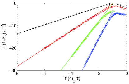
Figure 1: (Color online) Best-case performance for single-cycle DD under the CPMG (plus signs), PDD (circles), SDD (upward pointing triangles), and PCDD₂ (downward pointing triangles) protocol in the small $\tau$ region. Bath size $N=5$. Solid lines are linear fits, with fitting parameters given in Tab. 1.

Table 1 and Fig. 1 clearly demonstrate how DD performance improves as we go from PDD to SDD and to PCDD₂. Even though, as already remarked, the CPMG protocol $[C_{0}ZC_{0}Z]$ does not achieve maximal DD for zero bias field, the existence of an approximate integral of motion, $S_{z}$, still makes it possible to decouple with high fidelity provided that the initial electron spin state is a $S_{z}$-eigenstate. For two-axis cyclic DD, a preferred direction for initialization may still be identified. The PDD protocol $[C_{0}XC_{0}ZC_{0}XC_{0}Z]$, for instance, conserves $S_{y}$ in the limit $\tau\to 0$ (because $Z\,X\sim Y$, which coincides with the half-cycle direction); this establishes a $S_{y}$-eigenstate as the best-case state for PDD. When several DD cycles are implemented, the existence of approximate control-induced symmetries is responsible for the decoherence freezing phenomenon which we address next.

III.1.2 Long-time behavior

At long times, none of the above-mentioned analytical or symbolic methods is applicable, thus numerical simulation is required.

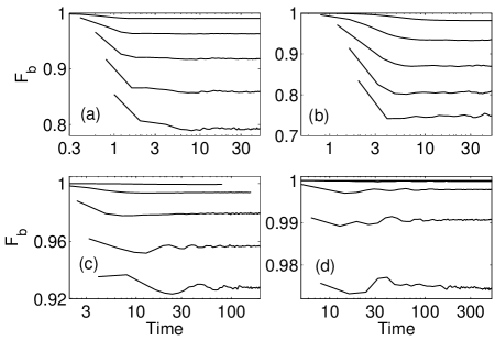
Figure 2: Best-case performance of (a) CPMG, (b) PDD, (c) SDD, and (d) PCDD₂ starting from an initial state along the half-cycle direction ($z$ for (a) and (c); $y$ for (b) and (d), respectively). Bath size: $N=15$. $\tau=0.1$, $0.2$, $0.3$, $0.4$, $0.5$, from top to bottom in all panels (in panel (d), the curves for $\tau=0.1$ and $0.2$ are indistinguishable). Decoherence freezes at sufficiently long time.

Fig. 2 shows the long-time best-case performance for the deterministic control protocols discussed so far. Decoherence freezing is clearly seen as a plateau of $F_{b}$ at sufficiently long evolution times Viola and Lloyd ; Zhang et al. (2007a), the corresponding saturation value increasing as the pulse delay $\tau$ decreases. From a control standpoint, decoherence freezing may be thought of as signaling the dynamical generation of a stable one-dimensional decoherence free subspace via DD Viola et al. (2000); Wu and Lidar (2002). In NMR language, the resulting saturation is reminiscent of the “pedestals” seen in the long-time magnetization signal under pulsed spin-locking conditions Haeberlen (1976); Suwelack and Waugh (1980); Ladd et al. (2005). Physically, one may think that an effective magnetic field is created by the DD pulses, and that proper alignment of the initial spin prevents the electron from precessing around this direction – thereby experiencing fully frozen nuclear spin fluctuations. (See also Ref. Oulton07, for a recent demonstration of a similar-in-spirit stabilization effect at zero applied field, leading to a long-lived nuclear-spin polaron state via optical pumping with polarized light). In practice, decoherence freezing may be exploited to optimally preserve a known initial electron spin state, through appropriate design of a DD protocol with the desired quasi-integral of motion. While a similar effect could be achieved by applying a strong static bias field, one advantage of DD stabilization is that better storage may be ensured by simply rearranging the pulse sequence, so that it implements a higher-level protocol (from PDD to PCDD₂, for example).

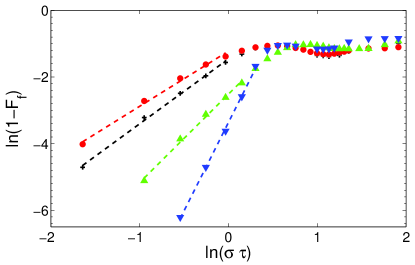
Figure 3: (Color online) Dependence of the coherence saturation value on pulse delay for CPMG (plus signs), PDD (circles), SDD (upward pointing triangles), and PCDD₂ (downward pointing triangles). Dashed lines are linear fittings at small $\tau$.

While asymptotic saturation behavior has been reported for purely dephasing spin-boson models with arbitrary initial spin states Viola and Lloyd (1998); Viola et al. (1999); Viola and Lloyd ; Shiokawa and Lidar (2004); Santos and Viola (2005), saturation effects for a spin bath have only received attention very recently Yao et al. (2007); Zhang et al. (2007a, ). Thanks to its inherent simplicity, the CPMG protocol makes it possible to gain analytical insight under the assumption that a simplified coupling Hamiltonian is appropriate:

$$H^{QSA}_{SB} = A{\mathbf{S}}\cdot\sum_{k=1}^{N}{\mathbf{I}}_{k}.$$ (25)

This corresponds to assuming a uniform electron density in the QD, allowing one to regard the total nuclear spin as a constant. For our purposes, because of the large number of spins in the bath, this is also equivalent to describing the nuclear spin reservoir under the so-called Quasi-Static Approximation (QSA), which treats the Overhauser nuclear field as a classical random static field Taylor et al. . While in principle the QSA is valid for short evolution times Taylor et al. ; Zhang et al. (2006), it is important to realize that the domain of validity of the QSA is extended in the presence of DD pulses, similarly to what happens for an external bias field Taylor et al. , and consistent with the fact that the nuclear field becomes progressively more static relative to the electron dynamics as the electron-nuclear coupling is suppressed.

By following the steps illustrated in Appendix A, the freezing value reported in Ref. Zhang et al., 2007a is obtained:

$$F_{f}^{\mbox{\small CPMG}}\approx 1-\frac{\tau^{2}}{2T_{2}^{*2}},$$

for sufficiently small $\tau$. Interestingly, the leading power of $\tau$, $n=2$, does not explicitly depend on the number $N$ of bath spins. For other protocols in the same range of $\tau$, numerical results (see Fig. 3) suggest a similar dependence of the asymptotic coherence value,

$$F_{f}\approx 1-a(\sigma\tau)^{n},\;\;\;a\in{\mathbb{R}},$$

with the relevant values of $n$ being given in Table 2. Note that the characteristic values of $\tau$ considered here are of order of $1/\sigma$, that is, $\omega_{c}\tau\gg 1$ in the simulations, thereby well beyond the convergence region of AHT/ME.

Table 2: Fitting parameters of the decoherence freezing value $F_{f}=1-a(\sigma\tau)^{n}$ for CPMG, PDD, SDD, and PCDD₂ at small $\tau$, where $\sigma\tau\lesssim 1$ but $\omega_{c}\tau\gg 1$.

	CPMG	PDD	SDD	PCDD2
$n({\rm Fit})$	2.0	1.7	2.7	5.3

III.2 Worst-case performance and arbitrary state preservation

As evidenced by the best-case considerations presented above, for sufficiently small $\tau$, initial electron spin states which are (approximate) eigenstates of the decoupled evolution are stable at long times, whereas the spin components perpendicular to the decoherence-free axis are lost in the long-time regime. In such a picture, the worst case scenario for a given cyclic protocol corresponds to initial spin states which are perpendicular to the effective half-cycle control axis. Clearly, worst-case performance lower-bounds the fidelity of storage achievable for an arbitrary (possibly unknown) initial state, as required for an electron-spin quantum memory.

III.2.1 Short-time behavior

In order to quantitatively assess worst-case DD fidelities, we begin, as in the previous Section, by examining single-cycle performance. Again, the order of the leading decoherence term is determined using three methods: (i) exact numerical simulation; (ii) analytical predictions based on AHT/ME; and (iii) symbolic Taylor expansion. Fig. 4 shows the exact $\tau$-dependence of the worst-case fidelity for single-cycle DD. Similar to the best case, $F_{w}(T_{c})$ depends on $\tau$ according to a power-law, when $\tau$ is sufficiently small to ensure that $\omega_{c}T_{c}\lesssim 1$ and that the AHT/ME approach is valid. Table 3 (first line) gives the leading decoherence term orders extracted from Fig. 4, which are in excellent agreement with the analytical and symbolic predictions (last two lines). Note that CPMG, which is not a universal decoupling sequence, is not useful in the worst-case scenario, thus we do not consider it further.

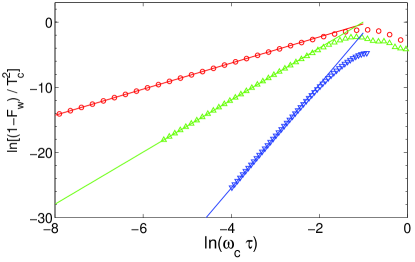
Figure 4: (Color online) Worst-case single-cycle performance for PDD (circles), SDD (upward pointing triangles), and PCDD₂ (downward pointing triangles) in the small $\tau$ region. Bath size: $N=5$. Solid lines are linear fittings, with fitting parameters given in Tab. 3.

Table 3: Fitting parameters of worst-case single-cycle performance $F_{w}(T_{c})=1-\kappa(\omega_{c}\tau)^{n}T_{c}^{2}$, $\kappa\in{\mathbb{R}}$, for PDD, SDD, and PCDD₂ in the small $\tau$ region where $\omega_{c}\tau\lesssim 1$.

	PDD	SDD	PCDD2
$n({\rm Fit})$	2.00	3.99	7.94
$n$(ME)	2	4	8
$n$(Sym)	2	4	8

III.2.2 Long-time behavior and randomized DD

For long evolution times, the worst-case performance $F_{w}(T)$ of six DD protocols (three deterministic and three randomized) are summarized in Fig. 5. All schemes lead to substantial enhancement of the electron spin coherence, some of them by more than a factor of 1000, with PCDD₂ showing the most dramatic improvement Zhang et al. (2007a). According to the ME, the leading order term for the FID signal is $\overline{\cal H}^{(0)}$, whereas it is $\overline{\cal H}^{(1)}$ for PDD, $\overline{\cal H}^{(2)}$ for SDD, and $\overline{\cal H}^{(4)}$ for PCDD₂, as discussed in Sec. II.2.2. For randomized protocols, lack of periodicity prevents the definition of a time-independent average Hamiltonian, thus AHT is not applicable. However, for a given evolution time, an effective Hamiltonian and the corresponding leading orders to coherence decay may still be defined directly in terms of the unitary logical-frame propagator Santos and Viola (2006); Santos06b .

In general, protocols with higher leading order tend to give superior performance. However, such a conclusion does not necessarily hold if a randomized protocol is compared to a deterministic one. For example, RPD has a lower-order leading term than SDD, so that SDD may outperform RPD at short times. However, Fig. 5 shows that at long times RPD outperforms SDD, which demonstrates the advantage of randomization in suppressing coherent error accumulation. The poor performance of NRD is expected, since the advantages of this low-level DD scheme may emerge only when ${\cal G}$ is large, and cyclic DD is inefficient. In a closed system Santos and Viola (2006), SRPD has been found superior to PCDD₂ at long times, but for the QD model considered here SRPD does not match PCDD₂, confirming the fact that irreducible DD groups and slow baths are especially favorable for concatenated control Khodjasteh and Lidar (2005). However, it is worth emphasizing that increase in the concatenation level for fixed pulse separation does not necessarily improve the protocol performance: As shown in Ref. Zhang et al., 2007a, PCDD₄ may deliver worse fidelity than PCDD₂ if $\tau$ becomes sufficiently large. A possible explanation may be rooted in the DD-induced renormalization of the pure-bath terms discussed in Sec. II.2.2, which for large $\tau$ may become important enough to offset the benefits associated with a more elaborated DD cycle.

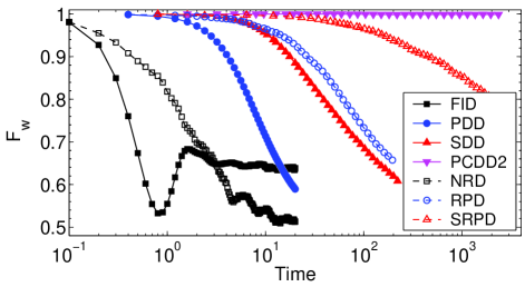
Figure 5: (Color online) Worst-case DD performance in the logical frame Viola and Knill (2005); Santos06b , with $\tau=0.1$. Hamiltonian parameters are: $\omega_{0}=0$, $\Gamma_{0}=0$ and $N=15$. For deterministic DD, data points are acquired at the completion of each cycle, while for NRD and FID this is done after every $\tau$, for RPD after every $4\tau$, and for SRPD after every $8\tau$. Random protocols are averaged over 100 control realizations.

IV Real-system considerations

In realistic scenarios, several factors beyond the simplified treatment considered thus far will unavoidably affect DD performance. Among those related to the underlying QD model Hamiltonian, the most important are the influence of spin-bath dynamics, external bias fields, and nuclear spin polarization. We shall address these factors one by one, by primarily focusing on the worst-case fidelity of the PCDD₂ protocol, which has emerged as the best performer for the problem under exam.

IV.1 Bath size

In our simulations, the number of bath spins is moderately large, $N\leq 25$, thus it is essential to assess to what extent our numerical results might be applicable to real QD devices with $N\sim 10^{4}$–$10^{6}$. In order to verify this, PCDD₂ simulations have been carried out for baths with $N$ varying from $15$ to $25$, their corresponding spectral width being characterized by $\sigma=\sqrt{N}A/2$ as in Eq. (20). Fig. 6 illustrates, for different $N$, the instant of time $T_{0.9}$ where $F_{w}(T)$ for PCDD₂ reaches a threshold value of $0.9$ – as a function of the dimensionless parameter $1/(2\sigma\tau)$. It is seen how, by correctly rescaling $\tau$ (that is, by measuring $\tau$ in units of $1/\sigma$), the curves corresponding to different bath size tend to fall on top of each other, especially as $N$ increases. This provides strong evidence that our results should be applicable to realistic mesoscopic spin environments upon appropriate parameter scaling.

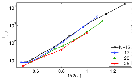
Figure 6: (Color online) Bath size effect. $T_{0.9}$ vs. $1/(2\sigma\tau)$ for PCDD₂ with different bath sizes $N=15$ (black squares), $17$ (blue circles), 20 (green upward pointing triangles), and $25$ (red downward pointing triangles).

It is also interesting to stress that $T_{0.9}$ increases extremely rapidly as the product $\sigma\tau$ decreases and the region of very fast DD is entered (note the logarithmic scale of the $y$-axis in Fig. 6). This rapid increase has been analyzed earlier Zhang et al. . We remark here that a naive extrapolation from the ME, $T_{0.9}\propto 1/\tau^{4}$, which could be expected to hold in the limit $\tau\rightarrow 0$, strongly disagrees with our data in the long-time parameter range of Fig. 6, and that a Zeno-type analysis as invoked in Ref. Zhang et al., appears more appropriate to explain the observed $\tau$-dependence.

IV.2 Intrabath interaction

The effect of the internal bath Hamiltonian $H_{B}$, Eq. (3), may become important once the electron coherence time becomes longer than the characteristic time scale of the corresponding bath evolution. As remarked, this effect may be enhanced in principle by the PCDD₂-induced pure-bath dipolar contribution, given in Eq. (17). In order to assess at which point DD performance start to be significantly affected by nuclear spin dynamics, we have performed numerical simulations by choosing $\Gamma_{kl}$ as uniformly random numbers in $[-\Gamma_{0},\Gamma_{0}]$, and by manually increasing $\Gamma_{0}$ up to values comparable to $0.1A_{k}$, to keep the simulation time reasonably short. In this way, in view of Eq. (18), we cause the effects of $H_{B}$ to be at least a factor of $3$ larger than the ones due to $\overline{H}^{(2)}$ for the maximum values of $\Gamma_{0}$ explored.

The results are summarized in Fig. 7, where a two-dimensional $4\times 5$ QD with nearest neighbor-intrabath coupling is considered. On one hand, the performance of PCDD₂ is affected only slightly for sufficiently small $\tau$ and $\Gamma_{0}$, as expected. Note that for a standard GaAs QD, the characteristic time scale for the nuclear spin dynamics is $\sim 100\mu$s, implying that $\Gamma_{0}\ll 0.01$ in our model. Thus, results obtained for $\Gamma_{0}=0$ are applicable to typical GaAs QDs. On the other hand, as it is also clear from Fig. 7, the long-time PCDD₂ fidelity deteriorates significantly in the presence of a sufficiently fast bath, especially for larger pulse delay $\tau$. Based on the spin-chain results of Ref. Santos and Viola, 2006, randomized protocols such as SRPD are capable to be, on average, more robust to the effects of the underlying bath evolution.

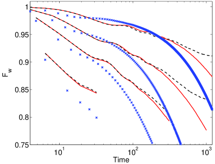
Figure 7: (Color online) Bath dynamics effect for PCDD₂ with $\Gamma_{0}=0$ (black dashed lines), $0.01$ (red solid lines), and $0.1$ (blue crosses). The parameters are $N=20$ and $\tau=0.2$, $0.25$, $0.3$, and $0.4$ from top to bottom.

IV.3 Magnetic bias field and initial bath polarization

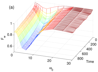
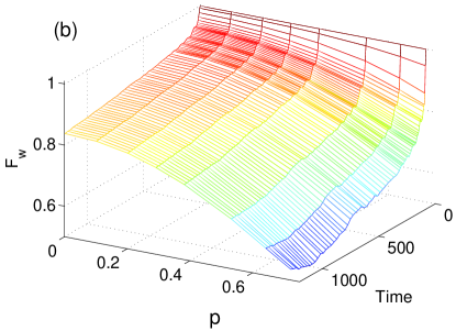
Figure 8: (Color online) Effect of bias magnetic field for different evolution times (top) and effect of initial bath polarization for (bottom) on the worst-case performance of PCDD₂. Parameters are $\tau=0.3$ and $N=15$. All energies are measured in units of $A$.

In practice, a non-zero Zeeman splitting in Eq. (2) might either be desirable in order to impose a controllable quantization axis on the electron spin and/or in any case result from residual magnetic fields in the device. As numerical results show (see Fig. 8(a)), the dependence of the PCDD₂ worst-case performance is non-monotonic with $B_{0}$, by decreasing with small magnetic fields and improving for large magnetic fields – this effect being more prominent for long evolution times. While this behavior is qualitatively consistent with the emergence of a predominantly pure-dephasing process in the presence of a strong bias field, the latter also leads, in general, to temporal modulation of the fidelity, similar to the effect of electron spin echo envelope modulation Rowan et al. (1965).

Interestingly, a non-zero initial polarization of the bath spins acts in a similar manner, see Fig. 8(b). In these simulations, we assumed that the initial state of the bath is described by a density matrix of the form

$$\rho_{B}(0)=\frac{1}{Z_{\beta}}e^{-\beta\sum_{k=1}^{N}I_{k}^{z}},\;\;\;Z_{\beta}=[2\cosh(\beta/2)]^{N},$$

where $\beta$ denotes as usual the inverse temperature. Accordingly, the bath polarization is defined as the ratio

$$p=\frac{1}{(N/2)}\sum_{k=1}^{N}\langle I_{k}^{z}\rangle=-\tanh(\beta/2),$$

with $\langle\cdot\rangle$ denoting the expectation over the above bath spin state. It has been shown earlier Zhang et al. (2006) that for the free decoherence dynamics of an electron spin in a QD, a non-zero Overhauser field produced by a small nuclear-spin polarization is essentially equivalent to an external bias field. Here, a similar equivalence emerges for the worst-case performance of PCDD₂: the degradation trend of the PCDD₂ fidelity for small polarizations seen in Fig. 8(b) resembles that occurring for small bias magnetic fields, $\omega_{0}\lesssim 4$. This indicates that the effect of the Overhauser field of a weakly polarized bath is also equivalent to that of an external bias field in the presence of DD pulses. We are unable to further explore this equivalence for larger values of the initial polarization, due to the fact that exact simulations with a highly polarized spin bath require numerical techniques which are beyond our current capabilities Zhang et al. (2007b). On physical grounds, we expect that the degradation trend should stop, and improved performance should emerge as $p$ approaches $1$, since the fidelity should achieve 100$\%$ for a fully polarized initial bath state (even in the absence of control pulses, for appropriate electron spin alignment).

V Control Resources

We conclude our analysis by addressing the main simplifying assumptions and requirements implicit in the control capabilities invoked so far, with respect to relevant practical constraints.

V.1 Effect of pulse imperfections

In all simulations presented thus far, control pulses have been assumed to exactly achieve a rotation angle of $\phi=\pi$ in no time – corresponding to zero width and infinite strength. In reality, pulses are clearly finite in both strength and width, and the implemented rotation angle typically deviates from the intended value due to both systematic control faults and stochastic parameter fluctuations. While a fully accurate error modelling is necessarily dependent upon the details of the physical implementation, our aim in what follows is to gain a sense on how stable PCDD₂ performance is in the presence of different representative control errors.

The effect of a systematic error in the rotation angle may be modelled by assuming that $\phi=\pi(1-\varepsilon)$, while keeping the pulse instantaneous, and letting $\varepsilon\in[0,1]$ represent the relative flip-angle error. Figure 9 summarizes numerical results for various error strengths. The protocol performance is not very sensitive to this type of error, especially for small $\varepsilon$ (as expected). In fact, the electron coherence time is still two orders of magnitude longer than $T_{2}^{*}$ even for $\varepsilon=0.03$, which corresponds to $\sim 5.4^{\circ}$. With phase compensation techniques Slichter (1992); Haeberlen (1976), DD performance might be further improved.

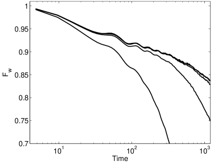
Figure 9: Effect of systematic rotation-angle errors on the worst-case PCDD₂ performance, with $\tau=0.3$ and $N=15$. The relative flip angle errors are $\varepsilon=0$, $0.001$ (indistinguishable from $\varepsilon=0$), $0.003$, $0.01$, $0.03$, from top to bottom.

The effect of finite pulse durations may be accounted for by assuming that each pulse is rectangular, with the width $w$ and the corresponding strength $\pi/w$ adjusted to represent an ideal $\pi$ pulse for an isolated spin. That is, the relevant control Hamiltonian becomes

$${H^{\prime}}_{c}(t)=\sum_{\ell}\frac{\pi}{w}({\bm{S}}\cdot\hat{\bm{n}}(t))[h(\ell\tau-t)-h(\ell\tau-t-w)],$$

where $h(\cdot)$ is the Heaviside step function. In simulations, we have considered the width of the pulse to be up to one third of the pulse delay, $w\leq\tau/3$. Figure 10 summarizes results on the worst-case PCDD₂ performance for different values of $w$: Clearly, DD performance depends quite sensitively on the pulse width. For a typical QD with decoherence time $T_{2}^{*}\sim 10$ ns, this means that pulse delays $\tau\sim 4$ ns and pulse widths no longer than $w=0.024$ (about $0.3$ ns) are required in order to extend $T_{2}^{*}$ by a factor of $\sim 100$ under PCDD₂.

Improved control design is needed to relax such stringent limitations, in particular to ensure that high-fidelity DD may be achieved with finite bandwidth. While further analysis along these lines is beyond our current scopes, preliminary results indicate how an approach based on Eulerian control Euler ; Viola (2004) may allow pulse widths as long as $\tau$ to be employed Taylor . A yet more sophisticated approach is to resort to numerical pulse shape optimization, for instance based on the recently proposed open-system gradient ascent pulse engineering algorithm Grape ; Wilhelm .

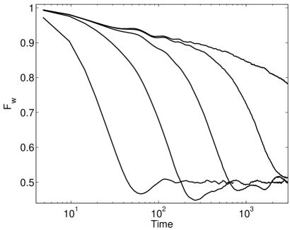
Figure 10: Effect of finite pulse width on the worst-case PCDD₂ performance, with $T_{c}=4.8=16\tau+20w$ and $N=15$. The pulse widths are $w=0$, $0.0024$, $0.008$, $0.024$, $0.08$, from top to bottom.

V.2 Feasibility considerations

From a practical standpoint, the main requirements for DD implementations are the ability to effect sufficiently fast single-spin rotations – along two orthogonal axes in an appropriate frame if storage of arbitrary electron spin states is sought. While this is a highly non-trivial task, single-spin rotations have by now been experimentally realized in both gate-defined radiofrequency-controlled GaAs double QDs Koppens et al. (2006) and self-assembled singly-charged (In,Ga)As/GaAs QDs Greilich et al. (2006); Dutt et al. (2006); Chen et al. (2004) – proposals for further improving rotation speed and gating time being actively investigated in parallel Emary and Sham (2007); Coish and Loss (2007). Likewise, multipulse CPMG protocols have been successfully implemented on single impurity centers in a solid-state matrix Fraval et al. (2005, 2004); Childress et al. (2006); HansonNV06 . In typical ESR settings, for instance, magnetic pulses as narrow as $20$ ns and gating times of the order of $100$ ns are currently attainable for typical GaAs QDs at dilution refrigerator temperatures Rim .

While the above-mentioned accomplishments and figures give hope that full-fledged DD experiments in QDs should become accessible in a near future, some additional remarks may be useful in connection with the prospective relevance of our results to different control implementations. Since, as remarked, our main focus has been on the zero-field limit ($\omega_{0}=0$), standard ESR techniques are not directly viable to effect the intended rotations. Rather, the control we are envisioning is based on direct magnetic switching, which may be accomplished in principle by having access to two independent inductances oriented along perpendicular axes. In order for the required control to be achievable via ESR or coherent Raman spectroscopy in the presence of a permanent static field, pulse widths and separations in the (sub)ns range would imply a resonance frequency $\omega_{0}\gtrsim 1$ GHz. In these conditions, as mentioned, the hyperfine decoherence process would be largely dephasing-dominated, and application of two-axis DD sequences such as PCDD₂ would result in even better performance than at zero field – similar to the conclusion reached in Sec. IV.3. As also noticed in Ref. Bergli and Glazman, , a potential advantage of control techniques not relying on the presence of an external field, however, is applicability over a wider range of parameters, along with the possibility to avoiding perturbations on the spin dynamics in between control operations. From this perspective, a more careful feasibility study of direct switching schemes in QD devices appears well-worth pursuing.

VI Conclusion

We have provided an in-depth quantitative analysis of the dynamical decoupling problem for a central spin system in the zero-field limit. While our main intended application has been long-time preservation of electron spin coherence in a quantum dot by suppression of hyperfine-induced coupling, we expect our main methods and conclusions to be relevant for control of nanospin systems described by a similar model Hamiltonian. Our main conclusions may be summarized as follows.

For short evolution times and inter-pulse delays $\tau$ which obey the condition $\omega_{c}\tau\lesssim 1$, $\omega_{c}$ being the spectral cut-off frequency of the total system, analytical results based on average Hamiltonian theory and the Magnus expansion are in excellent agreement with the results of exact numerical simulations. For longer evolution times and pulse separations, which are beyond the domain of applicability of analytical approaches, DD can still ensure high-fidelity preservation of arbitrary electron spin states, as long as typical control time scales are short with respect to the spectral width of the total system.

If knowledge of the initial electron state is available, cyclic DD protocols capable to completely freeze electron decoherence in the long-time limit may be designed – the attainable coherence value depending on both the protocol and the pulse delay.

By studying the effect of important experimental factors and control non-idealities – including the effect of intrabath interactions, external magnetic fields, and typical systematic pulse errors – we conclude that even imperfectly implemented decoupling protocols may still be able to significantly prolong the electron coherence time.

Appendix A Analytical Study of Decoherence Freezing Under CPMG Decoupling

The simplicity of the CPMG ($\tau Z\tau Z$) protocol allows for an analytical study of the saturation effect discussed in Sec. III.1. This will be done below via the QSA Taylor et al. ; Zhang et al. (2006), as well as based on a semiclassical random field model.

A.1 Quasi-Static Approximation

Within the QSA Taylor et al. ; Zhang et al. (2006), the Hamiltonian Eq. (1) reduces to $H_{A}$ Eq. (25). Let ${\mathbf{I}}=\sum_{k}{\mathbf{I}}_{k}$, and $M=I_{z}$. Due to the symmetry of $H_{A}$ and the CPMG protocol, ${\mathbf{I}}^{2}$ and $M+S_{z}$ are constants of motion. Let $|\Psi(0)\rangle=|\uparrow\rangle\otimes|I,M\rangle$ denote the the joint initial state, where the first ket-vector corresponds to the state of the electron spin and the second ket-vector denotes the state of the bath. Then the evolution of the controlled system only couples the pairs of levels $|\uparrow\rangle\otimes|I,M\rangle$ and $|\downarrow\rangle\otimes|I,M+1\rangle$. (Similar considerations apply to the case where the electron spin is down, initially).

After $n$ CPMG cycles, the evolution operator is

$$U(2n\tau) = \left(\begin{array}[]{cc}d_{1}&d_{2}^{*}\\ d_{2}&-d_{1}^{*}\end{array}\right)^{2n},$$

where we have defined

$$d_{1} = \cos{\Omega\frac{\tau}{2}}-i{\frac{B}{\Omega}}\sin{\Omega\frac{\tau}{2}},$$

$$d_{2} = -i{\frac{C}{\Omega}}\sin{\Omega\frac{\tau}{2}},$$

with $C=A\sqrt{(I-M)(I+M+1)}$, $B=A(M+1/2)$, and $\Omega^{2}=B^{2}+C^{2}$. In the best-case scenario, the overall system is initialized in the state

$$|\Psi(0)\rangle_{b}=|\uparrow\rangle\otimes|I,M\rangle,$$

whose survival probability is given by

$$|\langle\Psi(0)|\Psi(2n\tau)\rangle|^{2} = 1-{\frac{C^{2}}{B^{2}}}\tan^{2}\theta\cos^{2}2n\theta,$$

where $\tan\theta=d/\sqrt{1-d^{2}}$ with $d={\text{Im}}(d_{1})$.

The initial bath state is a completely mixed state and can be rewritten in the basis of $|I,M\rangle$ as

$$\rho_{B}(0) = \sum_{I,M}P(I,M)|I,M\rangle\langle I,M|,$$

with $P(I,M)\simeq(I/D\sqrt{2\pi D}\;)e^{-I^{2}/2D}$ for large $N$ and $D=N/4$ Melikidze et al. (2004). Averaging over the nuclear spin states, we obtain the survival probability, the input-output fidelity, at time $T=2n\tau$,

$$F(2n\tau) = 1-\int dIdMP(I,M){\frac{C^{2}}{B^{2}}}\tan^{2}\theta\cos^{2}2n\theta$$

$$= 1-\frac{1}{2}\int dIdMP(I,M){\frac{C^{2}}{B^{2}}}\tan^{2}\theta(1+\cos 4n\theta)$$

For $n$ large enough so that $4n\theta\gg 1$, we may safely neglect the contribution from rapidly oscillating part $\cos 4n\theta$. In these conditions, $F(2n\tau)$ becomes time-independent and decoherence is frozen,

$$F(2n\tau)\rightarrow F_{f} = 1-\frac{1}{2}\int dIdMP(I,M){\frac{C^{2}}{B^{2}}}\tan^{2}\theta.$$

In the limit of small $\tau$, this yields

$$F_{f}=1-\frac{1}{16}\tau^{2}A^{2}N=1-\frac{\tau^{2}}{2T_{2}^{*2}}.$$

For randomly distributed $A_{k}$, $A^{2}N\mapsto\sum_{k}A_{k}^{2}$.

For a single control cycle ($n=1$) as considered in Sec. III.1.1, and sufficiently small $\tau$ so that $\theta\ll 1$, it is straightforward to find that

$$F(T_{c}) = \frac{4}{5}-\frac{1}{15}\Big{[}(1-4D\tau^{2})e^{-2D\tau^{2}}$$

$$- 4(1-D\tau^{2})e^{-D\tau^{2}/2}\Big{]}$$

$$\approx 1-{\frac{D^{2}}{2}}\tau^{4}+{\mathcal{O}}(\tau^{6})=1-\kappa\tau^{2}T_{c}^{2}+{\mathcal{O}}(\tau^{4}T_{c}^{2}),$$

consistent with the result reported in the main text.

A.2 Classical Random Field Model

Yet another simple way to describe the saturation associated with the CPMG protocol at long times is as follows. In situations where the back-action effects from the system into the bath may be neglected, a plausible approximation is to treat the environment as a classical random field. This translates into rewriting the coupling Hamiltonian as

$$H=\vec{B}\cdot\vec{\sigma}\;,$$

where the effects of the randomly fluctuating field $\vec{B}$,

$$B_{x}=B\cos\theta\sin\phi,$$

$$B_{y}=B\sin\theta\sin\phi,$$

$$B_{z}=B\cos\phi,$$

are taken into account by averaging over the entire Bloch sphere of the system spin, $0\leq\phi\leq\pi$ and $0\leq\theta\leq 2\pi$.

Under CPMG, the unitary evolution after the completion of $n$ cycles may be written as

$$U(2n\tau) = \left(e^{-i(-B_{x}X-B_{y}Y+B_{z}Z)\tau}e^{-i(B_{x}X+B_{y}Y+B_{z}Z)\tau}\right)^{n}$$

$$= V\left(\begin{tabular}[]{cc}$e^{-i\lambda n}$&0\\ 0&$e^{i\lambda n}$\end{tabular}\right)V^{-1}\;,$$

where $V$ is the matrix of eigenvectors of $U(T_{c})$ and $\exp(\pm i\lambda)$, $\lambda\in{\mathbb{R}}$ denote the corresponding eigenvalues. For a particular initial state aligned with the dominant term of the AHT, that is $\overline{\cal H}^{(0)}=B_{z}Z$, the fidelity after $n$ cycles becomes

$$F_{b}(2n\tau)=\frac{\cos(B\tau)^{2}+\sin(B\tau)^{2}\sin(\phi)^{2}(1-\sin(n\lambda)^{2})}{\cos(B\tau)^{2}+\sin(B\tau)^{2}\sin(\phi)^{2}}\;.$$

In the long time limit, $n=t/(2\tau)\rightarrow\infty$, and upon averaging over $\theta$ and $\phi$, we finally obtain

$$F_{b}\rightarrow F_{f}=1-\frac{B^{2}\tau^{2}}{3}\;,$$

in agreement with the expression quoted in the main text.

Notice that the same result may also be obtained by restricting the analysis to the two dominant terms in the AHT (that is, $\overline{\cal H}^{(0)},\overline{\cal H}^{(1)}$) and by writing the propagator after $n$ cycles as

$$U(t=2n\tau)=e^{-i[B_{z}Zt+B_{z}(B_{x}Y-B_{y}X)t\tau]}.$$

While in principle no a priori reason exists to expect such AHT-based description to yield the correct answer, a similar treatment successfully describes long-time magnetization “pedestals” in NMR decoupling Haeberlen (1976).

References

- DiVincenzo (1995) D. P. DiVincenzo, Science 270, 255 (1995).
- (2) D. D. Awschalom, M. E. Flatté, N. Samarth, Scientific American 286, 66 (2002).
- (3) J. Baugh et al., e-print arXiv:quant-ph/0710.1447.
- Loss and DiVincenzo (1998) D. Loss and D. P. DiVincenzo, Phys. Rev. A 57, 120 (1998).
- Petta et al. (2005) J. R. Petta, A. C. Johnson, J. Taylor, E. A. Laird, A. Yacoby, M. D. Lukin, C. M. Marcus, M. P. Hanson, and A. C. Gossard, Science 309, 2180 (2005).
- Johnson et al. (2005) A. C. Johnson, J. R. Petta, J. M. Taylor, A. Yacoby, M. D. Lukin, C. M. Marcus, M. P. Hanson, and A. C. Gossard, Nature (London) 435, 925 (2005).
- Koppens et al. (2005) F. H. L. Koppens, J. A. Folk, J. M. Elzerman, R. Hanson, L. H. W. van Beveren, I. T. Vink, H. P. Tranitz, W. Wegscheider, L. P. Kouwenhoven, and L. M. K. Vandersypen, Science 309, 1346 (2005).
- Burkard et al. (1999) G. Burkard, D. Loss, and D. P. DiVincenzo, Phys. Rev. B 59, 2070 (1999).
- Deng and Hu (2006) C. Deng and X. Hu, Phys. Rev. B 73, 241303(R) (2006).
- (10) W. A. Coish and D. Loss, Phys. Rev. B 70, 195340 (2004).
- Stepanenko et al. (2006) D. Stepanenko, G. Burkard, G. Giedke, and A. Imamoglu, Phys. Rev. Lett. 96, 136401 (2006).
- (12) D. Klauser, W. A. Coish, and D. Loss, Phys. Rev. B 73, 205302 (2006).
- Gerstein and Dybowski (1985) B. C. Gerstein and C. R. Dybowski, Transient Techniques in NMR of Solids: An Introduction to Theory and Practice (Academic Press, Orlando, Florida, 1985).
- Haeberlen (1976) U. Haeberlen, High Resolution NMR in Solids: Selective Averaging (Academic Press, New York, 1976).
- Slichter (1992) C. P. Slichter, Principles of Magnetic Resonance (Springer-Verlag, New York, 1992).
- Viola and Lloyd (1998) L. Viola and S. Lloyd, Phys. Rev. A 58, 2733 (1998).
- Viola et al. (1999) L. Viola, E. Knill, and S. Lloyd, Phys. Rev. Lett. 82, 2417 (1999).
- Witzel and Sarma (2007) W. M. Witzel and S. Das Sarma, Phys. Rev. Lett. 98, 077601 (2007).
- Khodjasteh and Lidar (2005) K. Khodjasteh and D. A. Lidar, Phys. Rev. Lett. 95, 180501 (2005).
- (20) K. Khodjasteh and D. A. Lidar, Phys. Rev. A. 75, 062310 (2007).
- (21) J. Bergli and L. Glazman, Phys. Rev. B. 76, 064301 (2007).
- Yao et al. (2007) W. Yao, R.-B. Liu, and L. J. Sham, Phys. Rev. Lett. 98, 077602 (2007).
- Zhang et al. (2007a) W. Zhang, V. V. Dobrovitski, L. F. Santos, L. Viola, and B. N. Harmon, Phys. Rev. B 75, 201302(R) (2007a).
- (24) W. Zhang, V. V. Dobrovitski, L. F. Santos, L. Viola, and B. N. Harmon, J. Mod. Optics 54, 2629 (2007).
- Gaudin (1976) M. Gaudin, J. Phys. (Paris) 37, 1087 (1976).
- Prokof’ev and Stamp (2000) N. V. Prokof’ev and P. C. E. Stamp, Rep. Prog. Phys. 63, 669 (2000)
- Al-Hassanieh et al. (2006) K. A. Al-Hassanieh, V. V. Dobrovitski, E. Dagotto, and B. N. Harmon, Phys. Rev. Lett. 97, 037204 (2006).
- Dobrovitski and De Raedt (2003) V. V. Dobrovitski and H. A. De Raedt, Phys. Rev. E 67, 056702 (2003).
- Zhang et al. (2006) W. Zhang, V. V. Dobrovitski, K. A. Al-Hassanieh, E. Dagotto, and B. N. Harmon, Phys. Rev. B 74, 205313 (2006).
- (30) J. M. Taylor, J. R. Petta, A. C. Johnson, A. Yacoby, C. M. Marcus, and M. D. Lukin, Phys. Rev. B 76, 035315 (2007).
- (31) J. S. Hodges, J. C. Yang, C. Ramanathan, and D. G. Cory, arXiv:quant-ph/0707.2956.
- Paget et al. (1977) D. Paget, G. Lampel, B. Sapoval, and V. I. Safarov, Phys. Rev. B 15, 5780 (1977).
- Shenvi et al. (2005) N. Shenvi, R. de Sousa, and K. B. Whaley, Phys. Rev. B 71, 224411 (2005).
- de Sousa et al. (2005) R. de Sousa, N. Shenvi, and K. B. Whaley, Phys. Rev. B 72, 045330 (2005).
- (35) P. Zanardi, Phys. Lett. A 258, 77 (1999).
- (36) A. Iserleh and S. P. Norsett, Phil. Trans. R. Soc. A 357, 983 (1999); see also A. Iserleh, Notes of the AMS 49, 430 (2002).
- (37) E. Knill, R. Laflamme, and L. Viola, Phys. Rev. Lett. 84, 2525 (2000).
- (38) P. C. Moan and J. A. Oteo, J. Math. Phys. 42, 501 (2001).
- (39) M. M. Maricq, J. Chem. Phys. 86, 5647 (1987).
- Viola and Knill (2005) L. Viola and E. Knill, Phys. Rev. Lett. 94, 060502 (2005).
- (41) F. Casas, J. Phys. A 40, 15001 (2007).
- (42) The fact that the axis in preferred in the induced bath Hamiltonian (17) reflect the structure of the base sequence chosen for concatenation, which causes rotations to be comparatively more frequent, see Eq. (16).
- Kern and Alber (2005) O. Kern and G. Alber, Phys. Rev. Lett. 95, 250501 (2005).
- Santos and Viola (2006) L. F. Santos and L. Viola, Phys. Rev. Lett. 97, 150501 (2006).
- (45) L. Viola and L. F. Santos, J. Mod. Optics 53, 2559 (2006).
- Schumacher (1996) B. Schumacher, Phys. Rev. A 54, 2614 (1996).
- Nielsen (2002) M. A. Nielsen, Phys. Lett. A 303, 249 (2002).
- Fortunato et al. (2002) E. M. Fortunato, L. Viola, J. Hodges, G. Teklemariam, and D. G. Cory, New J. Phys. 4, 5 (2002).
- (49) A. J. Rimberg, Private comunication.
- Coish and Loss (2007) W. A. Coish and D. Loss, Phys. Rev. B 75, 161302(R) (2007).
- Zhang et al. (2007b) W. Zhang, N. P. Konstantinidis, K. A. Al-Hassanieh, and V. V. Dobrovitski, J. Phys.: Condens. Matter 19, 083202 (2007b).
- (52) S. Popescu, A. J. Short, and A. Winter, Nat. Phys. 2, 754 (2006).
- Nielsen and Chuang (2000) M. A. Nielsen and I. L. Chuang, Quantum Computations and Quantum Information (Cambridge University Press, Cambridge, 2000).
- (54) Since the order of the leading decoherence terms is independent of , we use the smallest possible bath size, , in implementing the expansion.
- Viola et al. (2000) L. Viola, E. Knill, and S. Lloyd, Phys. Rev. Lett. 85, 3520 (2000).
- Wu and Lidar (2002) L.-A. Wu and D. A. Lidar, Phys. Rev. Lett. 88, 207902 (2002).
- Suwelack and Waugh (1980) D. Suwelack and J. S. Waugh, Phys. Rev. B 22, 5110 (1980).
- Ladd et al. (2005) T. D. Ladd, D. Maryenko, Y. Yamamoto, E. Abe, and K. M. Itoh, Phys. Rev. B 71, 014401 (2005).
- (59) R. Oulton, A. Greilich, S. Yu. Verbin, R. V. Cherbunin, T. Auer, D. R. Yakovlev, M. Bayer, I. A. Merkulov, V. Stavarache, D. Reuter, and A. Wieck, Phys. Rev. Lett. 98, 107401 (2007).
- (60) L. Viola and S. Lloyd, e-print arXiv:quant-ph/9809058, in: Quantum Communication, Computing, and Measurement 2, P. Kumar, G. M. D’Ariano, and O. Hirota, Eds. (Plenum Publishing Co., New York, 2000), p. 59.
- Shiokawa and Lidar (2004) K. Shiokawa and D. A. Lidar, Phys. Rev. A 69, 030302(R) (2004).
- Santos and Viola (2005) L. F. Santos and L. Viola, Phys. Rev. A 72, 062303 (2005).
- Rowan et al. (1965) L. G. Rowan, E. L. Hahn, and W. B. Mims, Phys. Rev. 137, A61 (1965).
- (64) L. Viola and E. Knill, Phys. Rev. Lett. 90, 037901 (2003).
- Viola (2004) L. Viola, J. Mod. Opt. 51, 2357 (2004).
- (66) S. T. Smith, “Bounded-strength dynamical control of a single qubit based on Eulerian cycles,” Master Thesis, 2007 (unpublished).
- (67) T. Schulte-Herbrüggen, A. Spörl, N. Khaneja, and S. J. Glaser, e-print arXiv:quant-ph/0609037.
- (68) P. Rebentrost, I. Serban, T. Schulte-Herbrueggen, and F.K. Wilhelm, e-print arXiv:quant-ph/0612165.
- Koppens et al. (2006) F. H. L. Koppens, C. Buizert, K. J. Tielrooij, I. T. Vink, K. C. Nowack, T. Meunier, L. P. Kouwenhoven, and L. M. K. Vandersypen, Nature (London) 442, 766 (2006).
- Greilich et al. (2006) A. Greilich, R. Oulton, E. A. Zhukov, I. A. Yugova, D. R. Yakovlev, M. Bayer, A. Shabaev, A. L. Efros, I. A. Merkulov, V. Stavarache, et al., Phys. Rev. Lett. 96, 227401 (2006).
- Dutt et al. (2006) M. V. G. Dutt, J. Cheng, Y. Wu, X. Xu, D. G. Steel, A. S. Bracker, D. Gammon, S. E. Economou, R.-B. Liu, and L. J. Sham, Phys. Rev. B 74, 125306 (2006).
- Chen et al. (2004) P. Chen, C. Piermarocchi, L. J. Sham, D. Gammon, and D. G. Steel, Phys. Rev. B 69, 075320 (2004).
- Emary and Sham (2007) C. Emary and L. J. Sham, J. Phys.: Condens. Matter 19, 056203 (2007).
- Fraval et al. (2005) E. Fraval, M. J. Sellars, and J. J. Longdell, Phys. Rev. Lett. 95, 030506 (2005).
- Fraval et al. (2004) E. Fraval, M. J. Sellars, and J. J. Longdell, Phys. Rev. Lett. 92, 077601 (2004).
- Childress et al. (2006) L. Childress, M. V. G. Dutt, J. M. Taylor, A. S. Zibrov, F. Jelezko, J. Wrachtrup, P. R. Hemmer, and M. D. Lukin, Science 314, 281 (2006).
- (77) R. Hanson, F. M. Mendoza, R. J. Epstein, and D. D. Awschalom, Phys. Rev. Lett. 97, 087601 (2006).
- Melikidze et al. (2004) A. Melikidze, V. V. Dobrovitski, H. A. De Raedt, M. I. Katsnelson, and B. N. Harmon, Phys. Rev. B 70, 014435 (2004).