On the Linear Stability of Weakly-Ionized, Magnetized Planar Shear Flows

Abstract

We investigate the effects of ambipolar diffusion and the Hall effect on the stability of weakly-ionized, magnetized planar shear flows. Employing a local approach similar to the shearing-sheet approximation, we solve for the evolution of linear perturbations in both streamwise-symmetric and non-streamwise-symmetric geometries using WKB techniques and/or numerical methods. We find that instability arises from the combination of shear and non-ideal magnetohydrodynamic processes, and is a result of the ability of these processes to influence the free energy path between the perturbations and the shear. They turn what would be simple linear-in-time growth due to current and vortex stretching from shear into exponentially-growing instabilities. Our results aid in understanding previous work on the behaviour of weakly-ionized accretion discs. In particular, the recent finding that the Hall effect and ambipolar diffusion destabilize both positive and negative angular velocity gradients acquires a natural explanation in the more general context of this paper. We construct a simple toy model for these instabilities based upon transformation operators (shears, rotations, and projections) that captures both their qualitative and, in certain cases, exact quantitative behaviour.

1 Introduction

The importance of understanding the physics of shear flows has been appreciated for well over a century, starting with the pioneering work of von Helmholtz (1868) and Kelvin (1871). The stability of these flows in a wide variety of situations has been thoroughly studied and reviewed, most notably in Chandrasekhar’s (1961) classic text. Since that time, observations have revealed that shear flows are commonplace in astrophysical systems, playing likely roles in the stability and collimation of jets (e.g., Ferrari, Trussoni & Zaninetti, 1981; Fiedler & Jones, 1984; Begelman, Blandford & Rees, 1984), the solar corona (e.g., Karpen et al., 1993), bipolar outflows from young stellar objects (Pringle, 1989; Bachiller, 1996), rotating stars (Cowling, 1951; Goldreich & Schubert, 1967), accretion discs (Papaloizou & Lin, 1995; Balbus & Hawley, 1998), and even the Earth’s magnetopause (McKenzie, 1970). In nearly all of these systems, magnetic fields play a vital role in determining the structure and evolution. There are, however, systems where the importance of magnetic fields remain unclear, due to poor ionization and therefore weak coupling between the dominant ion and neutral species and the magnetic field. These include molecular clouds and their cores (Mouschovias & Ciolek, 1999), galactic molecular discs (Blaes & Balbus, 1994), protostellar accretion discs (Gammie, 1996; Hawley & Stone, 1998; Fromang, Terquem & Balbus, 2002), protostellar outflows and disc winds (Wardle & Königl, 1993), dwarf nova disks (Gammie & Menou, 1998; Sano & Stone, 2003), shock waves in dense molecular clouds (Wardle, 1991; Draine & McKee, 1993; Roberge & Ciolek, 2007), and protoplanetary discs (Sano & Miyama, 1999; Sano et al., 2000; Salmeron & Wardle, 2005; Chiang & Murray-Clay, 2007). In these systems, various non-ideal magnetohydrodynamic (MHD) effects may come into play. For example, the neutral particles may drift relative to the ions in a process referred to as ambipolar diffusion. If, on the other hand, the ions drift relative to the electrons (and thereby the magnetic field), then the Hall effect occurs.

Given the high occurrence of shear flows and low levels of ionization in various astrophysical environments, it is not surprising that examples can be found when the two coincide. Perhaps the most obvious examples are outflows from star-forming regions, where shear instabilities can occur at the interface between the jet and the ambient material (Watson et al., 2004). The resulting turbulent boundary layer can transfer linear momentum from the jet to the ambient medium, suggesting a possible mechanism for entrainment. Even at the launching point of these outflows, there may be differing velocity profiles in the ion and neutral fluids (see fig. 2 of Wardle & Königl 1993), conditions ripe for both ambipolar diffusion and shear. Another notable example concerns the interface between the magnetically-active and -inactive (‘dead’) regions in protoplanetary discs. It has been suggested that the well-coupled outer layers of protoplanetary discs will be subject to the magnetorotational instability (MRI; Balbus & Hawley 1991), while the shielded midplane layers will remain dormant (Gammie, 1996). In this situation, angular momentum can be effectively transported in the outer layers but not in the midplane, setting up a velocity profile in the vertical (away from the midplane) direction (Fleming & Stone, 2003; Fromang & Nelson, 2006).

Here we undertake a study of a magnetized, planar shear layer in the presence of ambipolar diffusion and the Hall effect, and find that instability arises when shear and non-ideal MHD effects act in concert. The instabilities are similar to those found by Wardle (1999), Balbus & Terquem (2001), Kunz & Balbus (2004), and Desch (2004) in the context of the MRI. Here we show that they are actually much more general. Our approach not only provides us with a clearer physical picture of the instabilities, free from the complications of rotation, but also brings qualitatively new results. In the case of ambipolar diffusion, instability arises from the combination of shear and the anisotropic nature of its wave damping. When the Hall effect is present, epicyclic-like motions set up by electromagnetic (whistler) waves couple to the background shear. When the handedness of these waves is opposite to that of the shear, instability occurs. It is notable that neither of these processes relies on rotational kinematics. In fact, these instabilities are neither versions of the Kelvin-Helmholtz instability (Watson et al., 2004), nor versions of the MRI (Balbus & Hawley, 1991, 1992b), despite their reliance on the presence of both shear and magnetic fields. The unstable modes are a result of the ability of non-ideal MHD processes to open new pathways for the fluid to tap into the free energy of shear.

An outline of the paper is as follows. In §2.1, we discuss the formulation of the problem and give the basic equations to be solved. We then consider the evolution of Eulerian perturbations to these equations in comoving, local Lagrangian coordinates (Goldreich & Lynden-Bell, 1965). After deriving two coupled equations for the evolution of the relevant magnetic field eigenvectors in §2.2, we solve them both analytically and numerically in several different situations. In §3, we first restrict our attention to the effects of ambipolar diffusion on the stability of the system. After a detailed analysis and discussion, we then examine the effects of Hall electromotive forces (HEMFs) in Section 4. Contact with prior work is emphasized. In §5, we construct and analyse a toy model that captures all the salient features of these instabilities. Section 6 summarizes our findings and conclusions.

2 Formulation of the Problem

2.1 Basic Equations

The equations describing a non-ideal MHD system, in the limit of negligible ion and electron inertia, are the continuity equation,

$$\frac{\partial\rho}{\partial t}+\mbox{\boldmath{$\nabla$}}\,\mbox{\boldmath{$\cdot$}}\,(\rho\mbox{\boldmath{$v$}})=0\,,$$ (1)

the force equation,

$$\frac{\partial\mbox{\boldmath{$v$}}}{\partial t}+\mbox{\boldmath{$v$}}\,\mbox{\boldmath{$\cdot$}}\,\mbox{\boldmath{$\nabla$}}\mbox{\boldmath{$v$}}=-\frac{1}{\rho}\mbox{\boldmath{$\nabla$}}P+\frac{\mbox{\boldmath{$j$}}\,\mbox{\boldmath{$\times$}}\,\mbox{\boldmath{$B$}}}{c\rho}\,,$$ (1)

the magnetic induction equation,

$$\frac{\partial\mbox{\boldmath{$B$}}}{\partial t}=\mbox{\boldmath{$\nabla$}}\,\mbox{\boldmath{$\times$}}\,\left[\mbox{\boldmath{$v$}}\,\mbox{\boldmath{$\times$}}\,\mbox{\boldmath{$B$}}-\frac{\mbox{\boldmath{$j$}}\,\mbox{\boldmath{$\times$}}\,\mbox{\boldmath{$B$}}}{en_{\rm e}}+\frac{(\mbox{\boldmath{$j$}}\,\mbox{\boldmath{$\times$}}\,\mbox{\boldmath{$B$}})\,\mbox{\boldmath{$\times$}}\,\mbox{\boldmath{$B$}}}{c\gamma\rho_{\rm i}\rho}\right]\,,$$ (1)

and Amperé’s law,

$$\mbox{\boldmath{$j$}}=\frac{c}{4\pi}\mbox{\boldmath{$\nabla$}}\,\mbox{\boldmath{$\times$}}\,\mbox{\boldmath{$B$}}\,.$$ (1)

Our notation is standard: $\rho$ is the mass density, $v$ is the velocity, $P$ is the gas pressure, $B$ is the magnetic field, and $j$ is the current density. The density, velocity, and pressure all refer to the dominant neutral species. The combination $\gamma\rho_{\rm i}$ is the neutral-ion collision frequency, with

$$\gamma=\frac{\langle\sigma w\rangle_{\rm in}}{m_{\rm i}+m_{\rm n}}$$

being the drag coefficient, and $n_{\rm e}$ the electron number density. The quantity $\langle\sigma w\rangle_{\rm in}$ is the average collisional rate between ions of mass $m_{\rm i}$ and neutrals of mass $m_{\rm n}$; it is equal to $1.69\times 10^{-9}\,(T/10\,{\rm K})^{1/2}$ cm³ s^-1 for HCO⁺-H₂ collisions, and is almost identical to this value for Na⁺-H₂ and Mg⁺-H₂ collisions (see McDaniel & Mason 1973).

The three terms on the right-side of Equation (1) represent induction, the Hall effect, and ambipolar diffusion, respectively. The difference between ion and electron velocities gives rise to the Hall effect, whereas the difference between ion and neutral velocities gives rise to ambipolar diffusion. Discussions of their relative magnitudes can be found in Balbus & Terquem (2001) and Sano & Stone (2002). For the sake of completeness, however, we repeat here the relative ratio of the ambipolar to Hall terms:

$$\frac{{\rm Am}}{{\rm Ha}}\sim\left(\frac{10^{13}\,{\rm cm}^{-3}}{n}\right)^{1/2}\,\left(\frac{T}{10^{3}\,{\rm K}}\right)^{1/2}\,\left(\frac{v_{\rm A}}{c_{\rm s}}\right)\,,$$ (2)

where $n$ is the number density of the neutrals and $c_{\rm s}$ is the isothermal sound speed. Assuming that the final two factors are each about 0.1, we see that a neutral density below about $10^{9}$ cm^-3 brings us safely into the ambipolar diffusion regime (see fig. 1 of Kunz & Balbus 2004). Since we are concerned here with the interplay between non-ideal MHD effects and shear, we ignore Ohmic dissipation, for which no shear instabilities are present. In writing Equation (1), we have implicitly assumed that the thermal-pressure force on the ions and electrons is negligible compared to the electromagnetic and collisional forces. This is an excellent approximation for the systems of interest. In addition, the inelastic momentum transfer by the ion and electron fluids due to attachment onto grains and neutralization is negligible compared to the momentum transfer due to elastic collisions, and it has been implicitly omitted from the induction equation. We have also ignored coupling via ionization and recombination, since these processes are slow compared to elastic processes.

Consider a flow in a stationary (‘lab’) Cartesian coordinate system along the $y$-axis, $\mbox{\boldmath{$v$}}=v(x)\hat{\mbox{\boldmath{$e$}}}_{y}$. Although we take the density and the magnetic field to be everywhere uniform, we put no restrictions on the $x$-dependance of the velocity field and the orientation of the magnetic field. Eulerian perturbations to this flow are allowed, denoted by a $\delta$. Keeping only terms linear in $\delta$ and working in the Boussinesq approximation, we find

$$\mbox{\boldmath{$\nabla$}}\,\mbox{\boldmath{$\cdot$}}\,\delta\mbox{\boldmath{$v$}}=0\,,$$ (3)

$$\frac{\partial\delta\mbox{\boldmath{$v$}}}{\partial t}+v(x)\frac{\partial\delta\mbox{\boldmath{$v$}}}{\partial y}+\hat{\mbox{\boldmath{$e$}}}_{y}\delta v_{x}\frac{dv(x)}{dx}=-\mbox{\boldmath{$\nabla$}}\left(\frac{\delta P}{\rho}+\frac{\mbox{\boldmath{$B$}}\,\mbox{\boldmath{$\cdot$}}\,\delta\mbox{\boldmath{$B$}}}{4\pi\rho}\right)+\frac{1}{4\pi\rho}(\mbox{\boldmath{$B$}}\,\mbox{\boldmath{$\cdot$}}\,\mbox{\boldmath{$\nabla$}})\delta\mbox{\boldmath{$B$}}\,,$$ (3)

$$\frac{\partial\delta\mbox{\boldmath{$B$}}}{\partial t}+v(x)\frac{\partial\delta\mbox{\boldmath{$B$}}}{\partial y}-\hat{\mbox{\boldmath{$e$}}}_{y}\delta B_{x}\frac{dv(x)}{dx}=(\mbox{\boldmath{$B$}}\,\mbox{\boldmath{$\cdot$}}\,\mbox{\boldmath{$\nabla$}})\delta\mbox{\boldmath{$v$}}-\left(\frac{c\mbox{\boldmath{$B$}}\,\mbox{\boldmath{$\cdot$}}\,\mbox{\boldmath{$\nabla$}}}{4\pi en_{\rm e}}\right)\,(\mbox{\boldmath{$\nabla$}}\,\mbox{\boldmath{$\times$}}\,\delta\mbox{\boldmath{$B$}})+\left(\frac{\mbox{\boldmath{$v_{\rm A}$}}\,\mbox{\boldmath{$\times$}}\,\mbox{\boldmath{$\nabla$}}}{\gamma\rho_{\rm i}}\right)\mbox{\boldmath{$\nabla$}}\,\mbox{\boldmath{$\cdot$}}\,(\mbox{\boldmath{$v_{\rm A}$}}\,\mbox{\boldmath{$\times$}}\,\delta\mbox{\boldmath{$B$}})+\frac{v^{2}_{\rm A}}{\gamma\rho_{\rm i}}\mbox{\boldmath{$\nabla$}}^{2}\delta\mbox{\boldmath{$B$}}\,,$$ (3)

where

$$\mbox{\boldmath{$v_{\rm A}$}}=\frac{\mbox{\boldmath{$B$}}}{(4\pi\rho)^{1/2}}$$

is the Alfvén velocity.

2.2 Shearing Sheet Formalism

The equations are first transformed from our lab-frame coordinate system to one comoving with the flow, centered at a fiducial location $(x_{0},y_{0},z_{0})$ moving at velocity $v(x_{0})=v_{0}$. We then consider a local neighborhood surrounding this point and Taylor expand the velocity field about $x_{0}$ to find

$$v(x)=v_{0}+(x-x_{0})\left.\frac{dv}{dx}\right|_{x_{0}}\,.$$

As is well known, a shearing background precludes simple plane wave solutions to the perturbation equations given in the previous section (Goldreich & Lynden-Bell, 1965). This difficulty is circumvented by adopting shearing coordinates, given by

$$x^{\prime}=x\,,$$ (4)

$$y^{\prime}=y-2Axt\,,$$ (4)

$$z^{\prime}=z\,,$$ (4)

$$t^{\prime}=t\,,$$ (4)

so that

$$\frac{\partial}{\partial x}=\frac{\partial}{\partial x^{\prime}}-2At^{\prime}\frac{\partial}{\partial y^{\prime}}\,,$$ (5)

$$\frac{\partial}{\partial y}=\frac{\partial}{\partial y^{\prime}}\,,$$ (5)

$$\frac{\partial}{\partial z}=\frac{\partial}{\partial z^{\prime}}\,,$$ (5)

$$\frac{\partial}{\partial t}=\frac{\partial}{\partial t^{\prime}}-2Ax^{\prime}\frac{\partial}{\partial y^{\prime}}\,,$$ (5)

where we have defined $2A\equiv(dv/dx)_{x_{0}}$. In this frame, the velocity field is $v(x^{\prime})=2Ax^{\prime}$. The benefit of this coordinate transformation is that a spatial dependence $\exp[i(k^{\prime}_{x}x^{\prime}+k^{\prime}_{y}y^{\prime}+k^{\prime}_{z}z^{\prime})]$ may be assumed for the perturbations, so long as we replace a fixed $x$ wavenumber with a shearing one:

$$k_{x}\leftarrow k_{x}(t)=k^{\prime}_{x}-2Ak^{\prime}_{y}t^{\prime}\,.$$ (6)

No modification of $y^{\prime}$ and $z^{\prime}$ variables are needed. Enacting this transformation and dropping the primes for ease of notation, our equations become

$$k_{x}\delta v_{x}+k_{y}\delta v_{y}+k_{z}\delta v_{z}=0\,,$$ (7)

$$\frac{d\delta v_{x}}{dt}+ik_{x}\left(\frac{\delta P}{\rho}+\frac{\mbox{\boldmath{$B$}}\,\mbox{\boldmath{$\cdot$}}\,\delta\mbox{\boldmath{$B$}}}{4\pi\rho}\right)-i\frac{\mbox{\boldmath{$k$}}\,\mbox{\boldmath{$\cdot$}}\,\mbox{\boldmath{$B$}}}{4\pi\rho}\,\delta B_{x}=0\,,$$ (7)

$$\frac{d\delta v_{y}}{dt}+2A\delta v_{x}+ik_{y}\left(\frac{\delta P}{\rho}+\frac{\mbox{\boldmath{$B$}}\,\mbox{\boldmath{$\cdot$}}\,\delta\mbox{\boldmath{$B$}}}{4\pi\rho}\right)-i\frac{\mbox{\boldmath{$k$}}\,\mbox{\boldmath{$\cdot$}}\,\mbox{\boldmath{$B$}}}{4\pi\rho}\,\delta B_{y}=0\,,$$ (7)

$$\frac{d\delta v_{z}}{dt}+ik_{z}\left(\frac{\delta P}{\rho}+\frac{\mbox{\boldmath{$B$}}\,\mbox{\boldmath{$\cdot$}}\,\delta\mbox{\boldmath{$B$}}}{4\pi\rho}\right)-i\frac{\mbox{\boldmath{$k$}}\,\mbox{\boldmath{$\cdot$}}\,\mbox{\boldmath{$B$}}}{4\pi\rho}\,\delta B_{z}=0\,,$$ (7)

$$\frac{d\delta B_{x}}{dt}-i(\mbox{\boldmath{$k$}}\,\mbox{\boldmath{$\cdot$}}\,\mbox{\boldmath{$B$}})\delta v_{x}-\frac{c(\mbox{\boldmath{$k$}}\,\mbox{\boldmath{$\cdot$}}\,\mbox{\boldmath{$B$}})}{4\pi en_{\rm e}}\,(\mbox{\boldmath{$k$}}\,\mbox{\boldmath{$\times$}}\,\delta\mbox{\boldmath{$B$}})_{x}+\frac{k^{2}v^{2}_{A}}{\gamma\rho_{\rm i}}\,\delta B_{x}-\frac{(\mbox{\boldmath{$k$}}\,\mbox{\boldmath{$\times$}}\,\mbox{\boldmath{$v_{\rm A}$}})_{x}}{\gamma\rho_{\rm i}}\,(\mbox{\boldmath{$k$}}\,\mbox{\boldmath{$\times$}}\,\mbox{\boldmath{$v_{\rm A}$}})\,\mbox{\boldmath{$\cdot$}}\,\delta\mbox{\boldmath{$B$}}=0\,,$$ (7)

$$\frac{d\delta B_{y}}{dt}-2A\delta B_{x}-i(\mbox{\boldmath{$k$}}\,\mbox{\boldmath{$\cdot$}}\,\mbox{\boldmath{$B$}})\delta v_{y}-\frac{c(\mbox{\boldmath{$k$}}\,\mbox{\boldmath{$\cdot$}}\,\mbox{\boldmath{$B$}})}{4\pi en_{\rm e}}\,(\mbox{\boldmath{$k$}}\,\mbox{\boldmath{$\times$}}\,\delta\mbox{\boldmath{$B$}})_{y}+\frac{k^{2}v^{2}_{A}}{\gamma\rho_{\rm i}}\,\delta B_{y}-\frac{(\mbox{\boldmath{$k$}}\,\mbox{\boldmath{$\times$}}\,\mbox{\boldmath{$v_{\rm A}$}})_{y}}{\gamma\rho_{\rm i}}\,(\mbox{\boldmath{$k$}}\,\mbox{\boldmath{$\times$}}\,\mbox{\boldmath{$v_{\rm A}$}})\,\mbox{\boldmath{$\cdot$}}\,\delta\mbox{\boldmath{$B$}}=0\,,$$ (7)

$$\frac{d\delta B_{z}}{dt}-i(\mbox{\boldmath{$k$}}\,\mbox{\boldmath{$\cdot$}}\,\mbox{\boldmath{$B$}})\delta v_{z}-\frac{c(\mbox{\boldmath{$k$}}\,\mbox{\boldmath{$\cdot$}}\,\mbox{\boldmath{$B$}})}{4\pi en_{\rm e}}\,(\mbox{\boldmath{$k$}}\,\mbox{\boldmath{$\times$}}\,\delta\mbox{\boldmath{$B$}})_{z}+\frac{k^{2}v^{2}_{A}}{\gamma\rho_{\rm i}}\,\delta B_{z}-\frac{(\mbox{\boldmath{$k$}}\,\mbox{\boldmath{$\times$}}\,\mbox{\boldmath{$v_{\rm A}$}})_{z}}{\gamma\rho_{\rm i}}\,(\mbox{\boldmath{$k$}}\,\mbox{\boldmath{$\times$}}\,\mbox{\boldmath{$v_{\rm A}$}})\,\mbox{\boldmath{$\cdot$}}\,\delta\mbox{\boldmath{$B$}}=0\,,$$ (7)

where the perturbations are now time-dependent Fourier amplitudes and we have suppressed the explicit time-dependent notation in $k_{x}$ and $k^{2}\equiv k^{2}_{x}+k^{2}_{y}+k^{2}_{z}$. Since $dk_{x}/dt=-2Ak_{y}$, Equations (7) - (7) together with Equation (7) guarantee the divergence free condition $d(\mbox{\boldmath{$k$}}\,\mbox{\boldmath{$\cdot$}}\,\delta\mbox{\boldmath{$B$}})/dt=0$.

In an attempt to keep the presentation as simple as possible, we first consider Equations (7) in the limit where ambipolar diffusion is the dominant non-ideal MHD process (§3), ignoring the Hall effect for the time being. Not only does this aid in our interpretation of the physics, but also the two processes generally act in distinct regions of parameter space. We then isolate the Hall effect in §4, neglecting ambipolar diffusion. The similarities and differences of the two resulting instabilities are discussed in Sections 5 and 6. Much of the formalism for understanding the Hall–shear instability is developed in the following section on ambipolar diffusion, and so it behooves us to encourage any readers primarily interested in Hall physics not to bypass the following section.

3 Ambipolar-Diffusion–Shear Instability

In this Section, we are concerned solely with the interplay of ambipolar diffusion and shear, and we neglect the Hall terms in Equations (7)-(7). Before we begin reducing these equations to a more manageable set, however, it is of interest to note that, while the presence of shear causes the $y$-component of the background magnetic field to grow linearly with time:

$$B_{y}(t)=B_{y}(0)+2AB_{x}t\,,$$

where $B_{y}(0)$ is the initial $y$ field, the combination $k$ $\cdot$ $B$ is constant with time, despite the fact that neither the Eulerian wavenumber $\mbox{\boldmath{$k$}}=[k_{x}(t),k_{y},k_{z}]$ nor the magnetic field vector $B$ is individually constant:

$$\mbox{\boldmath{$k$}}\,\mbox{\boldmath{$\cdot$}}\,\mbox{\boldmath{$B$}}=k^{\prime}_{x}B_{x}+k_{y}B_{y}(0)+k_{z}B_{z}\,.$$

Unfortunately, the same does not hold for the combination $k$ $\times$ $B$, and so the ambipolar diffusion terms in Equations (7)-(7) are intrinsically time-dependent. This complicates matters.

We simplify the set of Equations (7) as follows. Using $\mbox{\boldmath{$k$}}\,\mbox{\boldmath{$\cdot$}}\,\delta\mbox{\boldmath{$B$}}=0$, we first obtain

$$\delta B_{z}=-\frac{1}{k_{z}}\,\bigl{(}k_{x}\delta B_{x}+k_{y}\delta B_{y}\bigr{)}\,.$$ (8)

Then we may eliminate $\delta B_{z}$ from Equations (7) and (7) to find

$$\delta v_{x}=\frac{1}{i(\mbox{\boldmath{$k$}}\,\mbox{\boldmath{$\cdot$}}\,\mbox{\boldmath{$B$}})}\left[\left(\frac{d}{dt}+k^{2}\eta_{xx}\right)\delta B_{x}+k^{2}\eta_{xy}\delta B_{y}\right]\,,$$ (9)

$$\delta v_{y}=\frac{1}{i(\mbox{\boldmath{$k$}}\,\mbox{\boldmath{$\cdot$}}\,\mbox{\boldmath{$B$}})}\left[\left(\frac{d}{dt}+k^{2}\eta_{yy}\right)\delta B_{y}+\bigl{(}k^{2}\eta_{yx}-2A\bigr{)}\delta B_{x}\right]\,.$$ (9)

Here we have introduced the resistivity tensor $\eta$, whose elements are given by

$$\eta_{ij}=\frac{v^{2}_{\rm A}}{\gamma\rho_{\rm i}}\,\delta_{ij}-\frac{(\hat{\mbox{\boldmath{$k$}}}\,\mbox{\boldmath{$\times$}}\,\mbox{\boldmath{$v_{\rm A}$}})_{i}\,(\hat{\mbox{\boldmath{$k$}}}\,\mbox{\boldmath{$\times$}}\,\mbox{\boldmath{$v_{\rm A}$}})_{j}}{\gamma\rho_{\rm i}}+\frac{k_{j}}{k_{z}}\frac{(\hat{\mbox{\boldmath{$k$}}}\,\mbox{\boldmath{$\times$}}\,\mbox{\boldmath{$v_{\rm A}$}})_{i}\,(\hat{\mbox{\boldmath{$k$}}}\,\mbox{\boldmath{$\times$}}\,\mbox{\boldmath{$v_{\rm A}$}})_{z}}{\gamma\rho_{\rm i}}\,,$$ (10)

where $\delta_{ij}$ is the usual Kronecker delta function and $\hat{\mbox{\boldmath{$k$}}}$ is the unit wavevector. Next, we rearrange Equation (7):

$$\frac{\delta P}{\rho}+\frac{\mbox{\boldmath{$B$}}\,\mbox{\boldmath{$\cdot$}}\,\delta\mbox{\boldmath{$B$}}}{4\pi\rho}=\frac{1}{k_{y}(\mbox{\boldmath{$k$}}\,\mbox{\boldmath{$\cdot$}}\,\mbox{\boldmath{$B$}})}\left[\frac{d^{2}\delta B_{y}}{dt^{2}}+\frac{d}{dt}\bigl{(}k^{2}\eta_{yy}\delta B_{y}+k^{2}\eta_{yx}\delta B_{x}\bigr{)}+(\mbox{\boldmath{$k$}}\,\mbox{\boldmath{$\cdot$}}\,\mbox{\boldmath{$v_{\rm A}$}})^{2}\delta B_{y}+2A\bigl{(}k^{2}\eta_{xy}\delta B_{y}+k^{2}\eta_{xx}\delta B_{x}\bigr{)}\right]\,.$$ (11)

Inserting Equations (9) and (11) into Equation (7), we obtain

$$\frac{d^{2}\delta B_{x}}{dt^{2}}+\frac{d}{dt}\left(k^{2}\eta_{xx}\delta B_{x}-\frac{k_{x}}{k_{y}}k^{2}\eta_{yx}\delta B_{x}\right)+(\mbox{\boldmath{$k$}}\,\mbox{\boldmath{$\cdot$}}\,\mbox{\boldmath{$v_{\rm A}$}})^{2}\delta B_{x}-2A\frac{k_{x}}{k_{y}}\left(k^{2}\eta_{xx}+\frac{k_{y}}{k_{x}}k^{2}\eta_{yx}\right)\delta B_{x}$$ (12)

$$\mbox{}=\frac{k_{x}}{k_{y}}\left[\frac{d^{2}\delta B_{y}}{dt^{2}}+\frac{d}{dt}\left(k^{2}\eta_{yy}\delta B_{y}-\frac{k_{y}}{k_{x}}k^{2}\eta_{xy}\delta B_{y}\right)+(\mbox{\boldmath{$k$}}\,\mbox{\boldmath{$\cdot$}}\,\mbox{\boldmath{$v_{\rm A}$}})^{2}\delta B_{y}+2A\frac{k^{2}_{xy}}{k^{2}_{x}}k^{2}\eta_{xy}\delta B_{y}\right]\,.$$

For economy of notation, we have defined $k^{2}_{xy}\equiv k^{2}_{x}+k^{2}_{y}$. We need another independent differential equation coupling $\delta B_{x}$ and $\delta B_{y}$. Multiplying Equation (7) by $k_{z}$ and Equation (7) by $k_{y}$, then subtracting one from the other, we find

$$k_{z}\frac{d\delta v_{y}}{dt}+2Ak_{z}\delta v_{x}-k_{y}\frac{d\delta v_{z}}{dt}-ik_{z}\frac{\mbox{\boldmath{$k$}}\,\mbox{\boldmath{$\cdot$}}\,\mbox{\boldmath{$B$}}}{4\pi\rho}\,\delta B_{y}+ik_{y}\frac{\mbox{\boldmath{$k$}}\,\mbox{\boldmath{$\cdot$}}\,\mbox{\boldmath{$B$}}}{4\pi\rho}\,\delta B_{z}=0\,.$$ (13)

Using Equations (7), (8), and (9) in Equation (13) leads after some simplification to

$$\frac{d^{2}\delta B_{x}}{dt^{2}}+\frac{d}{dt}\left(k^{2}\eta_{xx}\delta B_{x}+\frac{k^{2}_{yz}}{k_{x}k_{y}}k^{2}\eta_{yx}\delta B_{x}\right)-4A\frac{k_{y}}{k_{x}}\frac{d\delta B_{x}}{dt}+(\mbox{\boldmath{$k$}}\,\mbox{\boldmath{$\cdot$}}\,\mbox{\boldmath{$v_{\rm A}$}})^{2}\delta B_{x}+2A\left(\frac{k^{2}_{z}-k^{2}_{y}}{k_{x}k_{y}}k^{2}\eta_{xx}-\frac{k^{2}_{yz}}{k^{2}_{x}}k^{2}\eta_{yx}\right)\delta B_{x}$$

$$\mbox{}=-\frac{k^{2}_{yz}}{k_{x}k_{y}}\left[\frac{d^{2}\delta B_{y}}{dt^{2}}+\frac{d}{dt}\left(k^{2}\eta_{yy}\delta B_{y}+\frac{k_{x}k_{y}}{k^{2}_{yz}}k^{2}\eta_{xy}\delta B_{y}\right)+(\mbox{\boldmath{$k$}}\,\mbox{\boldmath{$\cdot$}}\,\mbox{\boldmath{$v_{\rm A}$}})^{2}\delta B_{y}+2A\frac{k^{2}_{z}}{k^{2}_{yz}}k^{2}\eta_{xy}\delta B_{y}\right]\,.$$ (14)

Again, for economy of notation, we have defined $k^{2}_{yz}\equiv k^{2}_{y}+k^{2}_{z}$.

For numerical work, it is convenient to isolate the second-order time derivatives. Equations (12) and (3) may be recombined to yield

$$\frac{d^{2}\delta B_{x}}{dt^{2}}=-\frac{d}{dt}\bigl{(}k^{2}\eta_{xx}\delta B_{x}+k^{2}\eta_{xy}\delta B_{y}\bigr{)}+4A\frac{k_{x}k_{y}}{k^{2}}\frac{d\delta B_{x}}{dt}-(\mbox{\boldmath{$k$}}\,\mbox{\boldmath{$\cdot$}}\,\mbox{\boldmath{$v_{\rm A}$}})^{2}\delta B_{x}+4A\frac{k_{x}k_{y}}{k^{2}}\bigl{(}k^{2}\eta_{xx}\delta B_{x}+k^{2}\eta_{xy}\delta B_{y}\bigr{)}\,,$$ (15)

$$\frac{d^{2}\delta B_{y}}{dt^{2}}=-\frac{d}{dt}\bigl{(}k^{2}\eta_{yy}\delta B_{y}+k^{2}\eta_{yx}\delta B_{x}\bigr{)}+4A\frac{k^{2}_{y}}{k^{2}}\frac{d\delta B_{x}}{dt}-(\mbox{\boldmath{$k$}}\,\mbox{\boldmath{$\cdot$}}\,\mbox{\boldmath{$v_{\rm A}$}})^{2}\delta B_{y}-2A\frac{k^{2}_{xz}-k^{2}_{y}}{k^{2}}\bigl{(}k^{2}\eta_{xx}\delta B_{x}+k^{2}\eta_{xy}\delta B_{y}\bigr{)}\,.$$ (16)

Equations (15) and (16) are the two coupled differential equations in $\delta B_{x}$ and $\delta B_{y}$ that form the cornerstone of the analysis.

3.1 Qualitative Behavior

In a system where ambipolar diffusion and shear are absent, it is straightforward to show from Equations (15) and (16) that the perturbed magnetic field lines simply follow fluid elements, resulting in Doppler-shifted Alfvén waves propagating along the background magnetic field. The introduction of shear into the picture has two effects. The first effect is that vorticity is generated in the flow. The accompanying centrifugal force (associated with the resulting eddy) pushes on the shear interface, resulting in the growth of any deformation in the interface with time, provided that the vorticity is out of phase with the surface deformation. This is the essence of the Kelvin-Helmholtz instability. The second effect is that any $x$-displacement in the magnetic field becomes sheared out into an $y$-displacement. Thus, the perturbed magnetic field is effectively rotated until it becomes aligned with the shear interface.

In the presence of shear, any physical mechanism that conspires to rotate $\delta B_{y}$ back into $\delta B_{x}$ completes a feedback loop and results in growth. Ambipolar diffusion does just that. Since ambipolar diffusion only affects those currents flowing perpendicular to the background magnetic field, it tends to align magnetic field perturbations perpendicular to the background magnetic field. This manifests itself as an effective rotation of $\delta B_{y}$ into $\delta B_{x}$ (albeit with a decrease in $|\delta\mbox{\boldmath{$B$}}|$). In this case, ambipolar diffusion and shear conspire to stretch any perturbation in the magnetic field, resulting in an exponentially-growing instability. In a gas where either (1) the magnetic field is so strong that its tension effectively resists being stretched by the shear [i.e., $(\mbox{\boldmath{$k$}}\,\mbox{\boldmath{$\cdot$}}\,\mbox{\boldmath{$v_{\rm A}$}})^{2}\gg 4A^{2}$], or (2) the bulk neutral fluid is so poorly coupled to the magnetic field so that its velocity does not grow with it [i.e., $(\gamma\rho_{\rm i})\ll 2A$], this instability does not operate efficiently. We will show, however, that there still remains a great deal of unstable parameter space with which to work.

This route to instability has been seen before in the ambipolar-diffusion–modified MRI (Kunz & Balbus, 2004; Desch, 2004), where the role of shear is played by the differential rotation of an accretion disc [$v(x)=x\Omega(x)$, where $\Omega$ is the orbital frequency]. Here, however, we see that this destabilizing behaviour is part of a more general process, and in no way depends on rotational kinematics. The finding that ambipolar diffusion renders an accretion disc unstable (albeit weakly) for both inwardly- and outwardly-decreasing angular velocity profiles acquires a natural explanation in the more general context of this paper. Ambipolar diffusion can destabilize any shear flow profile, in very much the same way that the sign of $dv(x)/dx$ does not determine the outcome of the Kelvin-Helmholtz instability. In fact, we will show that the criterion for this ambipolar-diffusion shear instability is independent of the magnetic field strength, and is reliant only upon the ratio of the ion-neutral collision frequency $\gamma\rho_{\rm i}$ to the frequency implied by the shear of the flow, $2A$, and the geometry of the magnetic field.

3.2 The Case $k_{y}=B_{x}=0$: a Time-Independent Zero-Order State

The qualitative behaviour discussed above is most easily seen in the simple case of $k_{y}=B_{x}=0$. In this situation, the zero-order state is time-independent, and we may seek solutions to Equations (15) and (16) with time dependence $\exp(\sigma t)$. The resulting dispersion relation is

$$\sigma^{4}+\left[\frac{k^{2}v^{2}_{\rm A}+(\mbox{\boldmath{$k$}}\,\mbox{\boldmath{$\cdot$}}\,\mbox{\boldmath{$v_{\rm A}$}})^{2}}{\gamma\rho_{\rm i}}\right]\sigma^{3}+\mathcal{C}_{2}\sigma^{2}+(\mbox{\boldmath{$k$}}\,\mbox{\boldmath{$\cdot$}}\,\mbox{\boldmath{$v_{\rm A}$}})^{2}\left[\frac{k^{2}v^{2}_{\rm A}+(\mbox{\boldmath{$k$}}\,\mbox{\boldmath{$\cdot$}}\,\mbox{\boldmath{$v_{\rm A}$}})^{2}}{\gamma\rho_{\rm i}}\right]\sigma+\mathcal{C}_{0}=0\,,$$ (17)

where

$$\mathcal{C}_{2}=2(\mbox{\boldmath{$k$}}\,\mbox{\boldmath{$\cdot$}}\,\mbox{\boldmath{$v_{\rm A}$}})^{2}+\frac{k^{2}v^{2}_{\rm A}(\mbox{\boldmath{$k$}}\,\mbox{\boldmath{$\cdot$}}\,\mbox{\boldmath{$v_{\rm A}$}})^{2}}{(\gamma\rho_{\rm i})^{2}}-2A\,\frac{k_{x}B_{y}(\mbox{\boldmath{$k$}}\,\mbox{\boldmath{$\cdot$}}\,\mbox{\boldmath{$B$}})}{4\pi\gamma\rho_{\rm i}\rho}\,,$$ (18)

$$\mathcal{C}_{0}=(\mbox{\boldmath{$k$}}\,\mbox{\boldmath{$\cdot$}}\,\mbox{\boldmath{$v_{\rm A}$}})^{2}\left[(\mbox{\boldmath{$k$}}\,\mbox{\boldmath{$\cdot$}}\,\mbox{\boldmath{$v_{\rm A}$}})^{2}-2A\,\frac{k_{x}B_{y}(\mbox{\boldmath{$k$}}\,\mbox{\boldmath{$\cdot$}}\,\mbox{\boldmath{$B$}})}{4\pi\gamma\rho_{\rm i}\rho}\right]\,.$$ (18)

Before proceeding to obtain an instability criterion, let us note that Equation (17) may be written in the more compact form

$$\left[\sigma^{2}+\frac{k^{2}v^{2}_{\rm A}}{\gamma\rho_{\rm i}}\,\sigma+(\mbox{\boldmath{$k$}}\,\mbox{\boldmath{$\cdot$}}\,\mbox{\boldmath{$v_{\rm A}$}})^{2}\right]\,\left[\sigma^{2}+\frac{(\mbox{\boldmath{$k$}}\,\mbox{\boldmath{$\cdot$}}\,\mbox{\boldmath{$v_{\rm A}$}})^{2}}{\gamma\rho_{\rm i}}\,\sigma+(\mbox{\boldmath{$k$}}\,\mbox{\boldmath{$\cdot$}}\,\mbox{\boldmath{$v_{\rm A}$}})^{2}\right]=2A\,\frac{k_{x}B_{y}(\mbox{\boldmath{$k$}}\,\mbox{\boldmath{$\cdot$}}\,\mbox{\boldmath{$B$}})}{4\pi\gamma\rho_{\rm i}\rho}\bigl{[}\sigma^{2}+(\mbox{\boldmath{$k$}}\,\mbox{\boldmath{$\cdot$}}\,\mbox{\boldmath{$v_{\rm A}$}})^{2}\bigr{]}\,.$$ (19)

Consider the limit of vanishing shear. In this case, the right-hand side goes to zero and the two brackets on the left-hand side become decoupled from one another. The two solutions obtained by setting the left bracket to zero correspond to forward- and backward-propagating Alfvén waves with $\delta\mbox{\boldmath{$B$}}\,||\,\mbox{\boldmath{$B$}}$, which are damped at a rate $k^{2}v^{2}_{\rm A}/2\gamma\rho_{\rm i}$. The other two solutions obtained by setting the right bracket to zero correspond to forward- and backward-propagating Alfvén waves with $\delta\mbox{\boldmath{$B$}}\,||\,(\hat{\mbox{\boldmath{$k$}}}\,\mbox{\boldmath{$\times$}}\,\mbox{\boldmath{$B$}})$, which are damped at a rate $(\mbox{\boldmath{$k$}}\,\mbox{\boldmath{$\cdot$}}\,\mbox{\boldmath{$v_{\rm A}$}})^{2}/2\gamma\rho_{\rm i}$. One consequence of the difference in these damping rates is an effective rotation of $\delta\mbox{\boldmath{$B$}}\,\mbox{\boldmath{$\cdot$}}\,\mbox{\boldmath{$B$}}$ into $\delta\mbox{\boldmath{$B$}}\,\mbox{\boldmath{$\cdot$}}\,(\hat{\mbox{\boldmath{$k$}}}\,\mbox{\boldmath{$\times$}}\,\mbox{\boldmath{$B$}})$. As discussed in §3.1, this difference is at the heart of the ambipolar-diffusion–shear instability.

A sufficient condition for unstable solutions to exist in Equation (17) is $\mathcal{C}_{0}<0$, or

$$(\mbox{\boldmath{$k$}}\,\mbox{\boldmath{$\cdot$}}\,\mbox{\boldmath{$v_{\rm A}$}})^{2}-2A\,\frac{k_{x}B_{y}(\mbox{\boldmath{$k$}}\,\mbox{\boldmath{$\cdot$}}\,\mbox{\boldmath{$B$}})}{4\pi\gamma\rho_{\rm i}\rho}<0\,.$$ (20)

This is identical to the result in §4.2 of Kunz & Balbus (2004) in the limit of vanishing rotation frequency $\Omega$ (so that the epicyclic frequency $\kappa\rightarrow 0$), and is similar to the instability criterion for the ideal MRI (Balbus & Hawley, 1991):

$$(\mbox{\boldmath{$k$}}\,\mbox{\boldmath{$\cdot$}}\,\mbox{\boldmath{$v_{\rm A}$}})^{2}+\frac{k^{2}_{z}}{k^{2}}\frac{d\Omega^{2}}{d\ln R}<0\,.$$

Notice, however, that the stabilizing effects of ambipolar diffusion seen in the second term of equation (35) of Kunz & Balbus (2004) [which is $\propto\kappa^{2}(\mbox{\boldmath{$k$}}\,\mbox{\boldmath{$\cdot$}}\,\mbox{\boldmath{$v_{\rm A}$}})^{2}/(\gamma\rho_{\rm i})^{2}$] are absent here. This term represents epicyclic oscillations in the neutral fluid, an inherently stabilizing motion in Keplerian discs, being communicated to the (potentially) unstable ions through collisional coupling. In the limit $\gamma\rho_{\rm i}\rightarrow 0$ (i.e., infinite neutral-ion collision time-scale), it is clear that this term dominates and the bulk neutral fluid oscillates at the epicyclic frequency, unaffected by the presence of the magnetic field and the ions that are tied to it. In other words, if the neutrals can respond to magnetic forces on an epicyclic time-scale, the MRI will act on both fluids and will be effective in transporting angular momentum. Since it is rotation that gives birth to these stabilizing epicyclic oscillations, this term is absent in the dispersion relation given here. Evidentally, the situation investigated in both Kunz & Balbus (2004) and Desch (2004) was the superposition of two different, but related, instabilities acting in tandem: the MRI, whose magnetic ‘tether’ between fluid elements, essential to the transport of angular momentum, is undermined by the imperfect coupling between the ions and neutrals (leading to decreased growth rates); and an ambipolar-diffusion–shear instability, which results from the combination of shear and the anisotropic damping of ambipolar diffusion.

Further insight into the interpretation of Equation (20) is afforded by rewriting it in the form

$$\frac{2A}{\gamma\rho_{\rm i}}>\frac{k_{z}B_{z}}{k_{x}B_{y}}\,.$$ (21)

Note that the strength of the magnetic field is not at all relevant here; only the ratio of the shearing time-scale to the neutral-ion collision time-scale and the geometry of the magnetic field come into play. Furthermore, the freedom in choosing the sign of $k_{z}/k_{x}$ guarantees that any non-constant velocity profile can be destabilized, regardless of the sign of its derivative. Physically, this equation states that the time for a neutral particle to collide with an ion must be longer (by at least the factor given on the right-hand side) than the time it takes for a magnetic perturbation to grow by shear. If this condition is not met, the neutral fluid is well-coupled to the magnetic field, and we are left with simple linear-in-time growth due to shearing of the magnetic field perturbation.

Defining the dimensionless parameters,

$$X\equiv\frac{(\mbox{\boldmath{$k$}}\,\mbox{\boldmath{$\cdot$}}\,\mbox{\boldmath{$v_{\rm A}$}})^{2}}{4A^{2}}\quad\quad{\rm and}\quad\quad{\rm Am}\equiv\frac{|2A|}{\gamma\rho_{\rm i}}\,,$$ (22)

the dispersion relation may be written in dimensionless form and growth rates may be determined numerically. In Fig. 1, we give three-dimensional plots of growth rate in the $X$-$|k_{x}/k_{z}|$ plane (for ${\rm Am}=1$) and in the ${\rm Am}$-$|k_{x}/k_{z}|$ plane (for $X=1$). The signs of $k_{x}/k_{z}$ and $2A$ are chosen such that instability is possible, and $B_{y}/B_{z}$ is taken to be unity. Increasing $B_{y}/B_{z}$ does not significantly affect the growth rates, but rather opens the available unstable space to smaller values of ${\rm Am}$. Note that there is less unstable parameter space as one goes to small ${\rm Am}$ (the fluid becomes well-coupled to the magnetic field). The boundary separating stability from instability is given by Equation (21). The maximum growth rate ($\sim 0.1\,|2A|$; see Equation 33 below) is shown in Fig. 1c for the parameter space spanned by $X$ and ${\rm Am}$.

One final comment is worth mentioning concerning Equation (21). In a time-dependent zero-order state ($k_{y},B_{x}\neq 0$), the denominator of the right-hand side grows quadratic in time and the instability criterion will quickly become trivial to satisfy. It is therefore of interest to rigorously test whether this situation is realizable by performing an analysis of this more general case.

Figure 1: Counter-clockwise from top: ambipolar-diffusion–shear instability growth rates in (a) the $X$-$|k_{x}/k_{z}|$ plane with ${\rm Am}=1$ and (b) the ${\rm Am}$-$|k_{x}/k_{z}|$ plane with $X=1$; (c) maximum growth rates in the ${\rm Am}$-$X$ plane. All figures have $B_{y}/B_{z}=1$. Only regions of instability are shown, with the height being proportional to the growth rate. The maximum growth rate is $\sim 0.1\,|2A|$ (see Equation 33). Note that the boundary separating stability from instability is given by Equation (21).

3.3 The General Case

We now investigate the general case of mixed wavenumber and field geometry via two approaches. First, we employ a WKB technique. While this approach is strictly applicable only under special circumstances, it will aid in the interpretation of results from our second approach: a direct numerical solution of Equations (15) and (16).

3.3.1 WKB Analysis

Without loss of generality, one can express each perturbation variable in a WKB form:

$$\delta(t)\equiv\sum_{n=0}^{\infty}\delta^{(n)}(t)\exp\left(i\int\omega(t)dt\right)\,,$$ (23)

where the WKB phase has been expressed in terms of an integral over a slowly varying frequency. This is valid as long as $\delta^{(n+1)}\ll\delta^{(n)}$ and $d\ln\omega/dt\ll\omega$ (the adiabatic approximation). Both of these conditions are guaranteed if $k_{y}/k_{z}\ll 1$, and we may immediately identify the WKB parameter $k_{z}/k_{y}$. Physically, the WKB parameter represents the ratio of the time for $k$ to change significantly to the shearing time-scale. Expressing $\delta B_{x}$ and $\delta B_{y}$ in the form (23), taking the limit $k_{y}/k_{z}\rightarrow 0$, and defining $\sigma=i\omega$, the lowest-order terms from Equations (15) and (16) result in the following dispersion relation:

$$\sigma^{4}+k^{2}\,{\rm tr}(\mbox{\boldmath{$\eta$}})\sigma^{3}+\mathcal{C}_{2}\sigma^{2}+k^{2}\,{\rm tr}(\mbox{\boldmath{$\eta$}})\,(\mbox{\boldmath{$k$}}\,\mbox{\boldmath{$\cdot$}}\,\mbox{\boldmath{$v_{\rm A}$}})^{2}\sigma+\mathcal{C}_{0}=0\,,$$ (24)

where

$$\mathcal{C}_{2}=2(\mbox{\boldmath{$k$}}\,\mbox{\boldmath{$\cdot$}}\,\mbox{\boldmath{$v_{\rm A}$}})^{2}+k^{4}\det(\mbox{\boldmath{$\eta$}})+2Ak^{2}\eta_{xy}\,,$$ (25)

$$\mathcal{C}_{0}=(\mbox{\boldmath{$k$}}\,\mbox{\boldmath{$\cdot$}}\,\mbox{\boldmath{$v_{\rm A}$}})^{2}\bigl{[}(\mbox{\boldmath{$k$}}\,\mbox{\boldmath{$\cdot$}}\,\mbox{\boldmath{$v_{\rm A}$}})^{2}+2Ak^{2}\eta_{xy}\bigr{]}\,.$$ (25)

Here, ${\rm tr}(\mbox{\boldmath{$\eta$}})$ and $\det(\mbox{\boldmath{$\eta$}})$ denote the trace and determinant, respectively, of the resistivity tensor $\eta$. This is similar to the dispersion relation (17) in §3.2, and may be written in a form similar to that of Equation (19):

$$\left[\sigma^{2}+\sigma\Bigl{(}\;...\;\Bigr{)}_{+}+(\mbox{\boldmath{$k$}}\,\mbox{\boldmath{$\cdot$}}\,\mbox{\boldmath{$v_{\rm A}$}})^{2}\right]\left[\sigma^{2}+\sigma\Bigl{(}\;...\;\Bigr{)}_{-}+(\mbox{\boldmath{$k$}}\,\mbox{\boldmath{$\cdot$}}\,\mbox{\boldmath{$v_{\rm A}$}})^{2}\right]=-2Ak^{2}\eta_{xy}\bigl{[}\sigma^{2}+(\mbox{\boldmath{$k$}}\,\mbox{\boldmath{$\cdot$}}\,\mbox{\boldmath{$v_{\rm A}$}})^{2}\bigr{]}\,,$$ (26)

where

$$\Bigl{(}\;...\;\Bigr{)}_{\pm}=\frac{k^{2}{\rm tr}(\mbox{\boldmath{$\eta$}})}{2}\pm\left[\frac{k^{4}{\rm tr}^{2}(\mbox{\boldmath{$\eta$}})}{4}-k^{4}\det(\mbox{\boldmath{$\eta$}})\right]^{1/2}\,.$$ (26)

Evidently, the effect of shear is to couple different polarizations of Alfvén waves, which are damped at different rates. It is also of interest to calculate the associated eigenvectors. Defining

$$\tilde{\sigma}^{2}\equiv\sigma^{2}+k^{2}{\rm tr}(\mbox{\boldmath{$\eta$}})\sigma+k^{4}\det(\mbox{\boldmath{$\eta$}})+(\mbox{\boldmath{$k$}}\,\mbox{\boldmath{$\cdot$}}\,\mbox{\boldmath{$v_{\rm A}$}})^{2}+2Ak^{2}\eta_{xy}\,,$$ (27)

the (non-trivial) eigenvector components (in the limit $k_{y}/k_{z}\ll 1$) can be expressed as

$$\delta v_{y}=\frac{\delta v_{x}}{\sigma\tilde{\sigma}^{2}+k^{2}\eta_{xx}(\mbox{\boldmath{$k$}}\,\mbox{\boldmath{$\cdot$}}\,\mbox{\boldmath{$v_{\rm A}$}})^{2}}\,\bigl{[}-2A\tilde{\sigma}^{2}+(\mbox{\boldmath{$k$}}\,\mbox{\boldmath{$\cdot$}}\,\mbox{\boldmath{$v_{\rm A}$}})^{2}k^{2}\eta_{yx}\bigr{]}\,,$$ (28)

$$\delta B_{y}=\frac{-i(\mbox{\boldmath{$k$}}\,\mbox{\boldmath{$\cdot$}}\,\mbox{\boldmath{$B$}})\,\delta v_{x}}{\sigma\tilde{\sigma}^{2}+k^{2}\eta_{xx}(\mbox{\boldmath{$k$}}\,\mbox{\boldmath{$\cdot$}}\,\mbox{\boldmath{$v_{\rm A}$}})^{2}}\,\bigl{[}k^{2}\eta_{yx}\sigma+2Ak^{2}\eta_{xx}\bigr{]}\,,$$ (28)

$$\delta B_{x}=\frac{i(\mbox{\boldmath{$k$}}\,\mbox{\boldmath{$\cdot$}}\,\mbox{\boldmath{$B$}})\,\delta v_{x}}{\sigma\tilde{\sigma}^{2}+k^{2}\eta_{xx}(\mbox{\boldmath{$k$}}\,\mbox{\boldmath{$\cdot$}}\,\mbox{\boldmath{$v_{\rm A}$}})^{2}}\,\bigl{[}\sigma^{2}+k^{2}\eta_{yy}\sigma+(\mbox{\boldmath{$k$}}\,\mbox{\boldmath{$\cdot$}}\,\mbox{\boldmath{$v_{\rm A}$}})^{2}+2Ak^{2}\eta_{xy}\bigr{]}\,.$$ (28)

As in §3.2, a sufficient condition for instability is $\mathcal{C}_{0}<0$, or

$$(\mbox{\boldmath{$k$}}\,\mbox{\boldmath{$\cdot$}}\,\mbox{\boldmath{$v_{\rm A}$}})^{2}+2Ak^{2}\eta_{xy}<0\,.$$ (29)

This criterion depends on both $k_{x}(t)$ and $B_{y}(t)$, through $\eta_{xy}$. As a result, the destabilizing term will grow in amplitude, opening up more and more unstable parameter space as time progresses and increasing the growth rate.

If we view the dispersion relation (24) as an equation in $k^{2}$ and $(\mbox{\boldmath{$k$}}\,\mbox{\boldmath{$\cdot$}}\,\mbox{\boldmath{$v_{\rm A}$}})^{2}$, the maximum growth rate can be calculated for a given $\eta$. At the maximum growth rate $\sigma=\sigma_{\rm max}$, partial differentiation of Equation (24) with respect to $k^{2}$ and $(\mbox{\boldmath{$k$}}\,\mbox{\boldmath{$\cdot$}}\,\mbox{\boldmath{$v_{\rm A}$}})^{2}$ gives the two equations

$$k^{2}{\rm tr}(\mbox{\boldmath{$\eta$}})\sigma^{3}_{\rm max}+\bigl{[}2k^{4}\det(\mbox{\boldmath{$\eta$}})+2Ak^{2}\eta_{xy}\bigr{]}\sigma^{2}_{\rm max}+k^{2}{\rm tr}(\mbox{\boldmath{$\eta$}})\,(\mbox{\boldmath{$k$}}\,\mbox{\boldmath{$\cdot$}}\,\mbox{\boldmath{$v_{\rm A}$}})^{2}\sigma_{\rm max}+2Ak^{2}\eta_{xy}\,(\mbox{\boldmath{$k$}}\,\mbox{\boldmath{$\cdot$}}\,\mbox{\boldmath{$v_{\rm A}$}})^{2}=0\,,$$ (30)

$$2\sigma^{2}_{\rm max}+k^{2}{\rm tr}(\mbox{\boldmath{$\eta$}})\sigma_{\rm max}+2(\mbox{\boldmath{$k$}}\,\mbox{\boldmath{$\cdot$}}\,\mbox{\boldmath{$v_{\rm A}$}})^{2}+2Ak^{2}\eta_{xy}=0\,.$$ (31)

Eliminating $(\mbox{\boldmath{$k$}}\,\mbox{\boldmath{$\cdot$}}\,\mbox{\boldmath{$v_{\rm A}$}})^{2}$ between these two leads after regrouping to a surprisingly simple result,

$$\bigl{[}4\det(\mbox{\boldmath{$\eta$}})-{\rm tr}^{2}(\mbox{\boldmath{$\eta$}})\bigr{]}\sigma^{2}_{\rm max}-4A\eta_{xy}{\rm tr}(\mbox{\boldmath{$\eta$}})\sigma_{\rm max}-4A^{2}\eta^{2}_{xy}=0\,.$$ (32)

There are two solutions to this equation, corresponding to the extrema of the dispersion relation. Only one of these is a physically meaningful solution satisfying the dispersion relation (24); it is given by

$$\sigma_{\rm max}=|A|\,\left|\frac{\eta_{xy}}{\det^{1/2}(\mbox{\boldmath{$\eta$}})+\frac{1}{2}\,{\rm tr}(\mbox{\boldmath{$\eta$}})}\right|\,.$$ (33)

This is a remarkable result. Balbus & Hawley (1992a) conjectured that the maximum growth rate of any instability feeding off the differential rotation in a disc is given by the local Oort $A$ value, $\sigma_{\rm A}\equiv(1/2)|d\Omega/d\ln R|$, no matter the cause for instability. The reason is rooted in the dynamics of the differential rotation itself. In this paper, we are concerned with planar shear flows, and we arrive at a similar result, with the shear playing the role of the differential rotation. It is notable that Equation (33) is independent of the degree of ionization, depending only upon the geometry of the background magnetic field and the shearing rate $|2A|$.

The next order in a WKB expansion yields the time dependence of the slowly-varying amplitude. Provided we are able to compute this amplitude, the eigenvectors may be used to compute the wave energy and compare with the numerical results given in the next section. This has been done, e.g., by Johnson (2007) for the case of nonaxisymmetric shearing waves in differently-rotating disks. In a non-dissipative, continuous system, the amplitude may be computed from conservation of wave action. In the presence of ambipolar diffusion, however, wave action is not conserved, and retrieving the amplitude in this fashion is prohibitive. Instead, one must take the algebraically tedious approach of directly calculating the higher-order expansion for the modes. We have done this, finding an equation similar to that of equation (A5) of Johnson (2007). Unfortunately, once the eigenvectors (28) - (28) are substituted in, the result cannot be easily integrated and the slowly-varying amplitude cannot be calculated. Numerical solutions seem to be the most profitable approach.

3.3.2 Numerical Solution

Here we undertake a direct numerical solution of Equations (15) and (16). Following lines similar to those developed in Goldreich & Lynden-Bell (1965), we introduce a new independent time variable

$$\tau\equiv\frac{k_{x}(t)}{k_{z}}=\frac{k^{\prime}_{x}}{k_{z}}-2A\frac{k_{y}}{k_{z}}\,t\,,$$ (34)

so that $(k/k_{z})^{2}=\tau^{2}+(k_{y}/k_{z})^{2}+1$. Equations (15) and (16) may then be written in dimensionless form and numerically integrated. All that remains is to specify initial values for $\delta B_{x}$, $\delta B_{y}$, $\delta B_{z}$, and $B_{y}/B_{z}$. (The initial value of $\tau$ is determined from $\mbox{\boldmath{$k$}}\,\mbox{\boldmath{$\cdot$}}\,\delta\mbox{\boldmath{$B$}}=0$.) Unfortunately, we must also specify values for $k_{y}/k_{z}$ and $B_{x}/B_{z}$. However, we have undertaken a parameter study to see if varying these significantly influences the results, and have found that the qualitative behaviour is not affected. The results presented here have $\delta B_{x}(0)=0.3$, $\delta B_{y}(0)=\delta B_{z}(0)=0$, and $k_{y}/k_{z}=B_{x}/B_{z}=B_{y}(0)/B_{z}=1$.

In Fig. 2, we give the evolution of $\delta B_{x}$ (solid line) and $\delta B_{y}$ (dashed line) for (a) $(X,\,{\rm Am})=(1.0,\,1.0)$ , (b) $(X,\,{\rm Am})=(1.0,\,0.1)$, (c) $(X,\,{\rm Am})=(0.1,\,1.0)$, and (d) $(X,\,{\rm Am})=(0.1,\,0.1)$. Here, the sign of $2Ak^{\prime}_{x}/k_{z}$ is chosen to be negative so that the instability does not operate. The modes are damped due to ambipolar diffusion at a rate proportional to $2A/\gamma\rho_{\rm i}$ (i.e., a longer neutral-ion collision time-scale results in faster ambipolar diffusion). Decreasing $X$ results in a smaller damping rate (i.e., a longer Alfvén crossing time-scale allows more time for an ion to communicate the presence of the magnetic field to a neutral via collisions).

Figure 2: Evolution of the perturbed magnetic fields $\delta B_{x}$ (solid line) and $\delta B_{y}$ (dashed line) for (a) $(X,\,{\rm Am})=(1.0,\,1.0)$ , (b) $(X,\,{\rm Am})=(1.0,\,0.1)$, (c) $(X,\,{\rm Am})=(0.1,\,1.0)$, and (d) $(X,\,{\rm Am})=(0.1,\,0.1)$. The sign of $2Ak^{\prime}_{x}/k_{z}$ is chosen to be negative so that the flow is stable. The initial amplitudes are $\delta B_{x}=0.3$ and $\delta B_{y}=\delta B_{z}=0$, and $k_{y}/k_{z}=B_{x}/B_{z}=B_{y}(0)/B_{z}=1$. The initial value of $\tau=k^{\prime}_{x}/k_{z}$ is determined by $\mbox{\boldmath{$k$}}\,\mbox{\boldmath{$\cdot$}}\,\delta\mbox{\boldmath{$B$}}=0$.

Figure 3: Same as in Fig. 2, except that the sign of $2Ak^{\prime}_{x}/k_{z}$ is chosen to be positive so that the flow is unstable. Note that the ordinate value is $\ln|\delta B_{x}|$, rather than $\delta B_{x}$ as in Fig. 2. The evolution of $\delta B_{y}$ is similar and therefore not shown. There are, in general, two stages of evolution. Before the instability criterion is satisfied (i.e., $\tau=k_{x}(t)/k_{z}$ is too small) we have wave damping due to ambipolar diffusion. Once $\tau=k_{x}(t)/k_{z}$ reaches the value where Equation (29) is marginally satisfied, the growth phase begins.

In Fig. 3, we give the evolution of the corresponding unstable modes for the same parameters as in Fig. 2. The evolution of $\delta B_{y}$ in this case is similar to $\delta B_{x}$, and therefore is not given. Note that $\ln|\delta B_{x}|$ is plotted, rather than $\delta B_{x}$, so that the growth may be more clearly seen. There are, in general, two stages of evolution. Before the instability criterion is satisfied (i.e., $\tau=k_{x}(t)/k_{z}$ is too small) we have wave damping due to ambipolar diffusion (i.e., $\ln|\delta B_{x}|<0$). (The cusps on the plots correspond to the wave amplitude passing through zero and changing sign. For example, in Fig. 3b, the wave executes one full cycle before becoming unstable.) Once $\tau=k_{x}(t)/k_{z}$ reaches the value where Equation (29) is marginally satisfied, the growth phase begins (i.e., $\ln|\delta B_{x}|>0$).

Similar to investigations of other instabilities in the presence of a shearing time-dependent background (e.g., Balbus & Hawley 1992b, Balbus & Terquem 2001), we find that the evolution unfolds as a series of time-independent problems, whose analysis is aided by the existence of WKB solutions. Here, however, the analysis is complicated somewhat by the explicit time-dependence of the unstable terms. To keep things simple at first, consider the case $B_{x}=0$, so that the time-evolution of the destabilizing term is dependent only upon the wavenumber $k_{x}(t)(\,=k^{\prime}_{x}-2Ak_{y}t)$. In Fig. 4a we show the evolution of an initially leading wavenumber through the parameter space defined by ${\rm Am}$ and $|k_{x}/k_{z}|$ for $k_{y}/k_{z}=1$ and $B_{y}(\tau)=B_{y}(0)=0$. The wavevector evolution traces (and retraces) a horizontal line in the plane of Fig. 4a. In contrast to the nonaxisymmetric MRI (Balbus & Hawley, 1992b), the wavevector evolves towards stability, not away from it, and in principle spends only a finite amount of time in the stable region, that is, when $(\mbox{\boldmath{$k$}}\,\mbox{\boldmath{$\cdot$}}\,\mbox{\boldmath{$v_{\rm A}$}})^{2}>-2Ak^{2}\eta_{xy}$ is satisfied. In Fig. 4b, we relax our assumption of a vanishing $B_{x}$ and take $B_{x}/B_{z}=1$, so that $B_{y}$ is time-dependent. Recall that $k_{x}/k_{z}$ is our time parameter, so that $B_{y}$ increases with $k_{x}$. One modification to the picture presented in Fig. 4a is an extension of the unstable region at large $|k_{x}/k_{z}|$. This is due to the time-dependence of $B_{y}$ (and thereby, $\eta_{xy}$). Another important consequence is that, in principle, the growth rates will increase in time due to the fact that a strongly trailing (or leading) wavevector is trivially unstable. (These modes are well-localized in a WKB sense.) If the exponential growth phase goes unchecked by non-linear effects, it is conceivable that the growth rate will quickly surpass the shearing rate, or for that matter, any other dynamical rate in a system of interest.

Figure 4: (a) Regions of stability and instability in the ${\rm Am}$-$|k_{x}/k_{z}|$ plane for $B_{x}=0$. Initially, $|k_{x}/k_{z}|$ is large, and the point defining the wavevector moves to the left through the unstable region on a constant ${\rm Am}$ line. If $(\mbox{\boldmath{$k$}}\,\mbox{\boldmath{$\cdot$}}\,\mbox{\boldmath{$v_{\rm A}$}})^{2}>-2Ak^{2}\eta_{xy}$, then a finite portion of time is spent in the stable region. After attaining its minimum (i.e., $k_{x}/k_{z}=0$), the wavevector point retraces its path to the right, reentering the unstable region. (b) Same as in (a), but for $B_{x}/B_{z}=1$. See text for discussion.

One final issue remains: where does the energy come from to sustain this growth? The last term in Equation (29) introduces a novel form of coupling: in dyadic notation, it is

$$k^{2}\mbox{\boldmath{$\eta$}}\,\mbox{\boldmath{$:$}}\,\mbox{\boldmath{$\nabla$}}\,\mbox{\boldmath{$v$}}\,.$$

This suggests that ambipolar diffusion influences the free energy path between the velocity shear and the perturbations. In an ideal MHD shear flow, where ambipolar diffusion is absent, the link between the fluctuations and the free energy source is provided by vortex stretching. Magnetic fields modify this picture, of course, providing what amounts to an effective surface tension by resisting the shear. The effect of ambipolar diffusion may be most easily seen by using Equations (15) and (16) to derive an equation for

$$\delta J_{z}\equiv k_{x}\delta B_{y}-k_{y}\delta B_{x}\,,$$ (35)

which is proportional to the $z$-component of the perturbed current density:

$$\frac{1}{k_{x}}\left[\frac{d^{2}}{dt^{2}}+(\mbox{\boldmath{$k$}}\,\mbox{\boldmath{$\cdot$}}\,\mbox{\boldmath{$v_{\rm A}$}})^{2}\right]\delta J_{z}+\frac{4Ak_{y}}{k_{x}}\frac{d\delta B_{y}}{dt}$$ (36)

$$\mbox{}=-\frac{d}{dt}\bigl{(}k^{2}\eta_{yy}\delta B_{y}+k^{2}\eta_{yx}\delta B_{x}\bigr{)}+\frac{k_{y}}{k_{x}}\frac{d}{dt}\bigl{(}k^{2}\eta_{xx}\delta B_{x}+k^{2}\eta_{xy}\delta B_{y}\bigr{)}-2A\bigl{(}k^{2}\eta_{xx}\delta B_{x}+k^{2}\eta_{xy}\delta B_{y}\bigr{)}\,.$$

In the absence of ambipolar diffusion, the right-hand side vanishes, and we are left with a wave equation for $\delta J_{z}$ with the additional effect of shear acting as an amplitude modifier. The right-hand side is best approached piecemeal. The first two terms represent the damping of the current due to ambipolar diffusion. It is clear that different components of the perturbed current are damped differently. If ambipolar diffusion acted isotropically, with a resistivity $\eta\equiv\eta_{xx}=\eta_{yy}$, these terms would read

$$-\frac{1}{k_{x}}\frac{d}{dt}\,k^{2}\eta\delta J_{z}-\frac{2Ak_{y}}{k_{x}}\,k^{2}\eta\delta B_{y}\,,$$

which shows the effect of resistivity on the propagation of the wave, as well as the attempt to resist the stretching of the perturbed magnetic field by shear. The final term in Equation (36) is the key to instability. It becomes a source term when $k^{2}\mbox{\boldmath{$\eta$}}\,\mbox{\boldmath{$:$}}\,\mbox{\boldmath{$\nabla$}}\,\mbox{\boldmath{$v$}}<0$, extracting energy from the background velocity shear. In Fig. 5, we show the evolution of $\delta J_{z}$ for (a) $k^{2}\mbox{\boldmath{$\eta$}}\,\mbox{\boldmath{$:$}}\,\mbox{\boldmath{$\nabla$}}\,\mbox{\boldmath{$v$}}>0$ (stable), and (b) $k^{2}\mbox{\boldmath{$\eta$}}\,\mbox{\boldmath{$:$}}\,\mbox{\boldmath{$\nabla$}}\,\mbox{\boldmath{$v$}}<0$ (unstable). For the unstable case, the $z$-component of the vorticity ($\equiv k_{x}\delta v_{y}-k_{y}\delta v_{x}$) follows a similar evolution to the current.

Figure 5: Evolution of (a) $\delta J_{z}$ for $k^{2}\mbox{\boldmath{$\eta$}}\,\mbox{\boldmath{$:$}}\,\mbox{\boldmath{$\nabla$}}\,\mbox{\boldmath{$v$}}>0$ (stable), and (b) $\ln|\delta J_{z}|$ for $k^{2}\mbox{\boldmath{$\eta$}}\,\mbox{\boldmath{$:$}}\,\mbox{\boldmath{$\nabla$}}\,\mbox{\boldmath{$v$}}<0$ (unstable). Here, $(X,\,{\rm Am})=(1.0,\,1.0)$; initial values are as in Figures 2 and 3.

4 Hall–Shear Instability

We now consider the case where the Hall effect is the dominant non-ideal MHD process, corresponding to a neutral number density much in excess of $10^{13}$ cm^-3. The analysis follows the same course as in § 3, provided we redefine the resistivity tensor to be

$$k^{2}\mbox{\boldmath{$\eta$}}\rightarrow\frac{ck_{z}(\mbox{\boldmath{$k$}}\,\mbox{\boldmath{$\cdot$}}\,\mbox{\boldmath{$B$}})}{4\pi en_{\rm e}}\left(\begin{array}[]{rr}k_{x}k_{y}/k^{2}_{z}&k^{2}_{yz}/k^{2}_{z}\\ -k^{2}_{xz}/k^{2}_{z}&-k_{x}k_{y}/k^{2}_{z}\end{array}\right)\,.$$ (39)

Realizing that $k^{2}{\rm tr}(\mbox{\boldmath{$\eta$}})=0$ and $k^{4}\det(\mbox{\boldmath{$\eta$}})=c^{2}k^{2}(\mbox{\boldmath{$k$}}\,\mbox{\boldmath{$\cdot$}}\,\mbox{\boldmath{$B$}})^{2}/(4\pi en_{\rm e})^{2}$, the WKB dispersion relation (see §3.3.1) may immediately be written down:

$$\left[\sigma^{2}+i\,\sigma\frac{ck(\mbox{\boldmath{$k$}}\,\mbox{\boldmath{$\cdot$}}\,\mbox{\boldmath{$B$}})}{4\pi en_{\rm e}}+(\mbox{\boldmath{$k$}}\,\mbox{\boldmath{$\cdot$}}\,\mbox{\boldmath{$v_{\rm A}$}})^{2}\right]\left[\sigma^{2}-i\,\sigma\frac{ck(\mbox{\boldmath{$k$}}\,\mbox{\boldmath{$\cdot$}}\,\mbox{\boldmath{$B$}})}{4\pi en_{\rm e}}+(\mbox{\boldmath{$k$}}\,\mbox{\boldmath{$\cdot$}}\,\mbox{\boldmath{$v_{\rm A}$}})^{2}\right]=-2A\,\frac{ck_{z}(\mbox{\boldmath{$k$}}\,\mbox{\boldmath{$\cdot$}}\,\mbox{\boldmath{$B$}})}{4\pi en_{\rm e}}\bigl{[}\sigma^{2}+(\mbox{\boldmath{$k$}}\,\mbox{\boldmath{$\cdot$}}\,\mbox{\boldmath{$v_{\rm A}$}})^{2}\bigr{]}\,.$$ (40)

This is identical to equation (81) in Balbus & Terquem (2001) in the limit of vanishing rotation frequency $\Omega$ (and negligible Ohmic dissipation). Note that it is not necessary to assume $B_{y}/B_{x}\ll 1$, as in §3.3.1, since the only time-dependence is due to the wavenumber $k$ (recall that the combination $k$ $\cdot$ $B$ is a constant).

Before we proceed any further in analyzing Equation (40), it pays to examine the simple case of vanishing shear. The dispersion relation then becomes

$$\sigma^{2}\pm i\,\sigma\frac{ck(\mbox{\boldmath{$k$}}\,\mbox{\boldmath{$\cdot$}}\,\mbox{\boldmath{$B$}})}{4\pi en_{\rm e}}+(\mbox{\boldmath{$k$}}\,\mbox{\boldmath{$\cdot$}}\,\mbox{\boldmath{$v_{\rm A}$}})^{2}=0\,.$$ (41)

This is precisely the dispersion relation for a uniformly magnetized plasma with the displacement current and electron inertia ignored (see, e.g., Krall & Trivelpiece 1973); its positive frequency solutions are

$$\omega=-i\sigma=\mp\,\frac{ck(\mbox{\boldmath{$k$}}\,\mbox{\boldmath{$\cdot$}}\,\mbox{\boldmath{$B$}})}{8\pi en_{\rm e}}+\left[(\mbox{\boldmath{$k$}}\,\mbox{\boldmath{$\cdot$}}\,\mbox{\boldmath{$v_{\rm A}$}})^{2}+\frac{c^{2}k^{2}(\mbox{\boldmath{$k$}}\,\mbox{\boldmath{$\cdot$}}\,\mbox{\boldmath{$B$}})^{2}}{64\pi^{2}e^{2}n_{\rm e}^{2}}\right]^{1/2}\,.$$ (42)

For small wavenumbers (low frequencies), both of the above solutions reduce to Alfvén waves. At larger wavenumbers, however, right-handed waves (plus sign) go over to the high-frequency whistler wave branch, whereas large $k$ left-handed waves (minus sign) are cut off at a frequency

$$\omega_{\rm cutoff}=\frac{eB}{\mu c}\left(\frac{n_{\rm e}}{n}\right)\equiv\omega_{\rm c\mu}\left(\frac{n_{\rm e}}{n}\right)\,,$$ (43)

where $\mu$ is the mean mass per neutral particle. These modes arise due to the drift of the field lines with respect to the ion fluid as an Alfvén wave propagates through the lighter electron fluid, and are related to the so-called R- and L-waves of plasma physics.

Restoring the velocity shear, it is straightforward to show that instability proceeds through the point $\sigma=0$. The instability criterion is therefore

$$(\mbox{\boldmath{$k$}}\,\mbox{\boldmath{$\cdot$}}\,\mbox{\boldmath{$v_{\rm A}$}})^{2}+2A\,\frac{ck_{z}(\mbox{\boldmath{$k$}}\,\mbox{\boldmath{$\cdot$}}\,\mbox{\boldmath{$B$}})}{4\pi en_{\rm e}}<0\,.$$ (44)

This may be written in a more physically transparent form:

$$\frac{2A}{\omega_{\rm c\mu}}<-\frac{\mbox{\boldmath{$k$}}\,\mbox{\boldmath{$\cdot$}}\,\mbox{\boldmath{$B$}}}{k_{z}B}\left(\frac{n_{\rm e}}{n}\right)\,.$$ (45)

In other words, the time required for an ion to execute one orbital gyration around a magnetic field line must be longer (by at least the factor given on the right-hand side) than the time it takes for a magnetic perturbation to grow by shear. If this condition is not met, the ions are well-coupled to the electrons (and thereby the magnetic field), and we are left with simple linear-in-time growth due to shearing of the magnetic field perturbation. The freedom in choosing the sign of $k_{z}(\mbox{\boldmath{$k$}}\,\mbox{\boldmath{$\cdot$}}\,\mbox{\boldmath{$B$}})$ guarantees that any sign of shear can be destabilized, similar to the result in §3.2 involving ambipolar diffusion.

The maximum growth rate of this instability may be calculated directly from Equation (33):

$$\sigma_{\rm max}=|A|\,,$$ (46)

which occurs when $\mbox{\boldmath{$k$}}=k_{z}\hat{\mbox{\boldmath{$e$}}}_{z}$. This is in agreement with the findings of Balbus & Terquem (2001), despite our neglect of rotation. Defining the dimensionless parameters,

$$X\equiv\frac{(\mbox{\boldmath{$k$}}\,\mbox{\boldmath{$\cdot$}}\,\mbox{\boldmath{$v_{\rm A}$}})^{2}}{4A^{2}}\quad\quad{\rm and}\quad\quad{\rm Ha}\equiv\frac{1}{|2A|}\frac{ck_{z}(\mbox{\boldmath{$k$}}\,\mbox{\boldmath{$\cdot$}}\,\mbox{\boldmath{$B$}})}{4\pi en_{\rm e}}\,,$$ (47)

the dispersion relation may be written in dimensionless form and growth rates may be determined numerically. In Fig. 6, we give three-dimensional plots of growth rate in the $X$-$|k/k_{z}|$ plane (for $|{\rm Ha}|=2$) and in the $|{\rm Ha}|$-$|k/k_{z}|$ plane (for $X=1$). The signs of $k_{z}(\mbox{\boldmath{$k$}}\,\mbox{\boldmath{$\cdot$}}\,\mbox{\boldmath{$B$}})$ and $2A$ are chosen such that instability is possible, and $k_{y}$ is set to zero. Note that there is less unstable parameter space as one goes to small $|{\rm Ha}|$ (the ion-neutral fluid becomes well-coupled to the magnetic field). The maximum growth rate is shown in Fig. 6c for the parameter space spanned by $X$ and $|{\rm Ha}|$. It is important to notice that if a strongly-leading (or -trailing) wavevector ($|k/k_{z}|\gg 1$) begins its life in the unstable regime, it will always be unstable. By contrast, a stable wavevector will remain stable.

Figure 6: Counter-clockwise from top: hall–shear instability growth rates in (a) the $X$-$|k/k_{z}|$ plane with $|{\rm Ha}|=2$ and (b) the $|{\rm Ha}|$-$|k/k_{z}|$ plane with $X=1$; (c) maximum growth in the $X$-$|{\rm Ha}|$ plane. Only regions of instability are shown, with the height being proportional to the growth rate. The maximum growth rate is $|A|$.

We had argued earlier (see §3.1) that, in the presence of shear, any physical mechanism that conspires to rotate $\delta B_{y}$ back into $\delta B_{x}$ completes a feedback loop and results in growth. HEMFs accomplish this task not by preferential current damping, as in the case of the ambipolar-diffusion–shear instability, but rather by current generation. Consider the case of a purely vertical ($z$) wavenumber and magnetic field. The effect of shear on the background magnetic field and the coordinate system vanishes, and we may write down the linearized induction Equations (7) and (7) in the form

$$\frac{d\delta B_{x}}{dt}+\frac{ck_{z}(\mbox{\boldmath{$k$}}\,\mbox{\boldmath{$\cdot$}}\,\mbox{\boldmath{$B$}})}{4\pi en_{\rm e}}\,\delta B_{y}=i(\mbox{\boldmath{$k$}}\,\mbox{\boldmath{$\cdot$}}\,\mbox{\boldmath{$B$}})\delta v_{x}\,,$$ (48)

$$\frac{d\delta B_{y}}{dt}-\left[\frac{ck_{z}(\mbox{\boldmath{$k$}}\,\mbox{\boldmath{$\cdot$}}\,\mbox{\boldmath{$B$}})}{4\pi en_{\rm e}}+2A\right]\delta B_{x}=i(\mbox{\boldmath{$k$}}\,\mbox{\boldmath{$\cdot$}}\,\mbox{\boldmath{$B$}})\delta v_{y}\,.$$ (48)

We assume that instability is possible, i.e., that the Hall and shear terms in Equation (48) have opposite signs. It is clear from Equation (48) that shear uses $\delta B_{x}$ to generate a $\delta B_{y}$. The Hall terms, on the other hand, generate $\delta B_{x}$ at the expense of $\delta B_{y}$. This effect is actually present in the absence of shear, and arises because the $y$-component of the perturbed electron velocity differs from the ion-neutral velocity (recall that ambipolar diffusion is ignored here) by a term involving $\delta J_{y}(\equiv k_{z}\delta B_{x}-k_{x}\delta B_{z})$. The induced magnetic field is sheared further, leading to runaway. This behaviour can be seen differently by viewing the Hall terms as ‘Coriolis’ terms in the magnetic field equations. These give birth to magnetic ‘epicycles’, i.e., circularly-polarized electromagnetic waves. When the sign of the rotation imparted by the shear is opposite to that of the handedness of these waves, a struggle ensues over control of the direction of the perturbed magnetic field vector. For every bit of field line stretching in the $y$ direction due to shear, Hall forces rotate this increased field back into the $x$ direction, only to be stretched further by shear. The compromise of this struggle is an exponentially-growing instability.

This route to instability has been seen before in the Hall-modified MRI (Wardle, 1999; Balbus & Terquem, 2001), where the role of shear is played by the differential rotation of an accretion disc [$v(x)=x\Omega(x)$, where $\Omega$ is the orbital frequency]. In that case, however, the behaviour of the Hall terms is complicated by rotation, which influences the magnetic epicycles by introducing a sense of helicity (see section 3 of Balbus & Terquem 2001 for a discussion). The finding that HEMFs render an accretion disc unstable for both inwardly- and outwardly-decreasing angular velocity profiles does not depend on rotational kinematics. Rather, it is a simple result of the influence of shear on the propagation of circularly-polarized electromagnetic waves.

At this point a few questions naturally emerge. First, why does the Hall–shear instability require a vertical $(z)$ wavenumber in order to operate, whereas the ambipolar-diffusion–shear instability does not? Simply put, the interaction between shear and the Hall effect is strongest when the motions implied by the shear lie in the same plane as the magnetic “epicycles” induced by the Hall effect. In other words, instability is maximized when the vorticity $\mbox{\boldmath{$\Gamma$}}\equiv\mbox{\boldmath{$\nabla$}}\,\mbox{\boldmath{$\times$}}\,\mbox{\boldmath{$v$}}$, the wavevector $k$, and the magnetic field $B$ all share a mutual axis. Translated mathematically, this implies that the relevant Hall term is $(\mbox{\boldmath{$k$}}\,\mbox{\boldmath{$\cdot$}}\,\mbox{\boldmath{$B$}})(\mbox{\boldmath{$k$}}\,\mbox{\boldmath{$\cdot$}}\,\mbox{\boldmath{$\Gamma$}})$; it must be negative for destabilization. This is distinct from the findings of Wardle (1999) and Balbus & Terquem (2001), who found that the relevant coupling parameter is, respectively, $(\mbox{\boldmath{$\Omega$}}\,\mbox{\boldmath{$\cdot$}}\,\mbox{\boldmath{$B$}})$ or $(\mbox{\boldmath{$k$}}\,\mbox{\boldmath{$\cdot$}}\,\mbox{\boldmath{$B$}})(\mbox{\boldmath{$k$}}\,\mbox{\boldmath{$\cdot$}}\,\mbox{\boldmath{$\Omega$}})$ where $\Omega$ is the rotation vector. This corroborates our finding that the Hall instability is not a result of differential rotation per se, but rather of any source of shear. Our coupling parameter matches theirs when the vorticity shares the same axis as the rotation, a situation typical for disc systems. Second, why is the growth rate for the Hall–shear instability typically so much greater than for the ambipolar-diffusion–shear instability? Both processes involve extraction of free energy from the background shear flow. The reason lies in the fact that the Hall effect employs a conservative process (cyclotron gyrations) rather than a dissipative process (ambipolar diffusion) to rotate $\delta B_{y}$ back into $\delta B_{x}$. Not surprisingly, the difference in the growth rates is related to the rate at which the gas is heated due to ion-neutral friction.

5 Discussion: Shears, Rotations, and Projections

Despite the impression one may get from the abundance of mathematical manipulations in the preceding sections, the instabilities themselves are actually quite simple. They are the result of combinations of shears, rotations (in the case of the Hall effect), and projections (in the case of ambipolar diffusion). Much in the way that the MRI may be understood by two orbiting masses connected by a spring (Balbus & Hawley, 1992a), there exists an equally intuitive toy model that captures the essence of the shear instabilities examined in this paper. Through simple matrix multiplication, several main results can be recovered without recourse to the lengthy mathematical manipulations undertaken in the preceding sections. All we require is some linear algebra.

Consider the following abstract problem, in which a position vector $|r_{0}\rangle=|x_{0},y_{0}\rangle$ (in Dirac notation), having the coordinates $[x_{0},y_{0}]$ in a two-dimensional $x$-$y$ Cartesian coordinate system, is subjected to various shear, rotation, and projection operators given by

$$\mbox{\boldmath{$\mathsf{S}$}}\equiv\left[\begin{array}[]{cc}1&0\\ \varepsilon&1\\ \end{array}\right]\,,\qquad\mbox{\boldmath{$\mathsf{R}$}}\equiv\left[\begin{array}[]{rr}\cos\theta&-\sin\theta\\ \sin\theta&\cos\theta\\ \end{array}\right]\,,\qquad{\rm and}\qquad\mbox{\boldmath{$\mathsf{P}$}}\equiv\left[\begin{array}[]{cc}\sin^{2}\phi&-\sin\phi\cos\phi\\ -\sin\phi\cos\phi&\cos^{2}\phi\\ \end{array}\right]\,,$$ (49)

respectively. We denote by the column vector $|r_{n}\rangle=|x_{n},y_{n}\rangle$ the position vector $|r\rangle$ after $n$ transformations have been applied to $|r_{0}\rangle$. To be precise, the combination $\mbox{\boldmath{$\mathsf{S}$}}|r\rangle$ results in a shearing of $|r\rangle$ along the $y$-axis by a distance $\varepsilon x$; $\mbox{\boldmath{$\mathsf{R}$}}|r\rangle$ results in a counter-clockwise rotation of $|r\rangle$ through an angle $\theta$; and, $\mbox{\boldmath{$\mathsf{P}$}}|r\rangle$ projects $|r\rangle$ onto the unit vector $|-\sin\phi,\cos\phi\rangle$. These will be put in a physical context below.

We first turn our attention to the shear and projection operators. Applying the combination $\mathsf{S}$$\mathsf{P}$ (a projection followed by shear) to the initial state vector $|r_{0}\rangle$ advances it to $|r_{1}\rangle$:

$$|r_{1}\rangle=\mbox{\boldmath{$\mathsf{SP}$}}|r_{0}\rangle=(x_{0}\sin\phi-y_{0}\cos\phi)\left[\begin{array}[]{c}\sin\phi\\ \varepsilon\sin\phi-\cos\phi\\ \end{array}\right]\,.$$ (50)

A graphical depiction of this process is given in Fig. 7. While $|r_{0}\rangle$ is clearly not an eigenvector of the operator $\mathsf{SP}$, it is straightforward to show that $|r_{1}\rangle$ is an eigenvector, with eigenvalue $(1-\varepsilon\sin\phi\cos\phi)$. It is then trivial to write down the result for general $n\geq 1$:

$$|r_{n}\rangle=(1-\varepsilon\sin\phi\cos\phi)\,|r_{n-1}\rangle=(1-\varepsilon\sin\phi\cos\phi)^{n-1}\,|r_{1}\rangle\,.$$ (51)

Put differently, after this transformation has been performed just once, all subsequent applications simply stretch (or contract) the vector along $|r_{1}\rangle$ by a factor equal to the associated eigenvalue. Note that in order for any evolution to occur, $\phi\neq m\pi/2$ with $m$ an integer. For growth, we require

$$\varepsilon\sin\phi\cos\phi<0\,.$$ (52)

We now place these results in the context of the ambipolar-diffusion–shear instability. With $\varepsilon=2A\Delta t$ and $|r\rangle=\delta\mbox{\boldmath{$B$}}$, our shear operator corresponds physically to the production of $\delta B_{y}$ due to the shearing of $\delta B_{x}$ in a time $\Delta t$. When $\phi$ is taken to be the angle between a background magnetic field and the $x$-axis, the projection operator embodies ambipolar diffusion acting on the vector $|r\rangle=\delta\mbox{\boldmath{$B$}}$. Their combination leads precisely to the behaviour described in §3.1. In fact, it embodies the exact solution for the case $\mbox{\boldmath{$k$}}=k_{z}\hat{\mbox{\boldmath{$e$}}}_{z}$ and $\mbox{\boldmath{$B$}}=B\cos\phi\hat{\mbox{\boldmath{$e$}}}_{x}+B\sin\phi\hat{\mbox{\boldmath{$e$}}}_{y}$, as can be readily verified by taking the limit $\Delta t\rightarrow 0$ in Equation (51) to arrive at the differential equation:

$$\frac{dr}{dt}=-A\sin(2\phi)\,r\,.$$ (53)

If $A\sin(2\phi)<0$, we have exponential growth. The growth rate is $A\sin(2\phi)$, which has its maximum at precisely the Oort $A$ value. That the maximum growth rate occurs at $\phi=\pi/4$ is in accord with the well-known “$\sin\,2l$” law (e.g., Mihalas & Binney 1981), a result of particular significance; we refer the reader to §2.4 of Balbus & Hawley (1992a) for a full discussion of this topic.

Next we turn our attention to the shear and rotation operators. Applying the combination $\mathsf{S}$$\mathsf{R}$ (a rotation followed by shear) to the initial state vector $|r_{0}\rangle$ advances it to $|r_{1}\rangle$:

$$|r_{1}\rangle=\mbox{\boldmath{$\mathsf{SR}$}}|r_{0}\rangle=(x_{0}\sin\theta-y_{0}\cos\theta)\left[\begin{array}[]{c}1\\ \varepsilon\\ \end{array}\right]+(x_{0}\sin\theta+y_{0}\cos\theta)\left[\begin{array}[]{c}0\\ 1\\ \end{array}\right]\,.$$ (54)

A graphical depiction of this process is given in Fig. 8. For $n\geq 2$, it is possible to show that a recursion relation exists between successive state vectors:

$$|r_{n}\rangle-(2\cos\theta-\varepsilon\sin\theta)|r_{n-1}\rangle+|r_{n-2}\rangle=0\,.$$ (55)

This equation has the general solution:

$$|r_{n}\rangle=\left(\frac{\lambda^{n}_{+}-\lambda^{n}_{-}}{\lambda_{+}-\lambda_{-}}\right)\,|r_{1}\rangle-\left(\frac{\lambda^{n-1}_{+}-\lambda^{n-1}_{-}}{\lambda_{+}-\lambda_{-}}\right)\,|r_{0}\rangle\,,$$ (56)

where

$$\lambda_{\pm}=\left(\cos\theta-\frac{\varepsilon}{2}\sin\theta\right)\pm\left[\left(\cos\theta-\frac{\varepsilon}{2}\sin\theta\right)^{2}-1\right]^{1/2}$$ (57)

are the characteristic roots of Equation (55). With $\theta=\omega\Delta t$ and $|r\rangle=\delta\mbox{\boldmath{$B$}}$, this transformation corresponds to the physical behaviour described in §4 concerning the evolution circularly-polarized electromagnetic waves (with frequency $\omega$) in the presence of shear; namely, in a time $\Delta t$, the perturbed magnetic field vector is rotated by $\mathsf{R}$ through an angle $\omega\Delta t$ and sheared by $\mathsf{S}$ along the $y$-axis. Taking the $\Delta t\rightarrow 0$ limit of Equation (55) gives the differential equation

$$\frac{d^{2}r}{dt^{2}}=-\omega(\omega+2A)\,r\,,$$ (58)

whose solutions are exponentially growing if

$$\frac{2A}{\omega}<-1\,.$$ (59)

The similarity between this instability criterion and Equation (45) is striking. When $|A/\omega|$ equates to unity, the growth rate attains its maximum value: precisely the Oort $A$ constant. This simple model captures all the salient features of the Hall–shear instability.

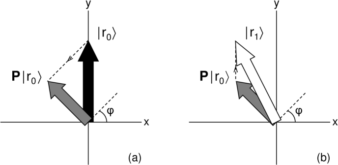
Figure 7: Evolution of the initial state vector $|r_{0}\rangle$ (solid arrow) under the transformation $\mathsf{SP}$. (a) A projection is applied to $|r_{0}\rangle$ that retains only its component lying along the unit normal $|-\sin\phi,\cos\phi\rangle$. The result is $\mbox{\boldmath{$\mathsf{P}$}}|r_{0}\rangle$ (grey arrow). (b) This vector is then sheared along the $y$-axis into $|r_{1}\rangle$ (open arrow). This process represents the ambipolar-diffusion–shear instability (see text for details). Figure is drawn to scale for comparison with Fig. 8.

Figure 8: Evolution of the initial state vector $|r_{0}\rangle$ (solid arrow) under the transformation $\mathsf{SR}$. (a) A counter-clockwise rotation by $\theta$ is applied to $|r_{0}\rangle$, taking it into $\mbox{\boldmath{$\mathsf{R}$}}|r_{0}\rangle$ (grey arrow). (b) This vector is then sheared along the $y$-axis into $|r_{1}\rangle$ (open arrow). The process represents the Hall–shear instabiliy (see text for details). Figure is drawn to scale for comparison with Fig. 7.

6 Summary

In this paper, we have investigated the stability of weakly-ionized, magnetized planar shear flows to linear disturbances. Employing a local approach similar to the shearing-sheet approximation of Goldreich & Lynden-Bell (1965), we have derived two coupled differential equations governing the evolution of magnetic field perturbations in the presence of either ambipolar diffusion or the Hall effect. Solutions are found by WKB methods and by direct numerical integration. We find that instability arises from the combination of shear and non-ideal MHD processes, and is a result of the ability of these processes to open new pathways for the fluid to feed off the free energy of shear. They turn what would be simple linear-in-time growth due to current and vortex stretching from shear into exponential instabilities. We have also constructed a simple toy model based on transformation operators that not only captures all the qualitative results of this paper, but also matches the exact quantitative solution in some specific instances.

In the case of ambipolar diffusion, anisotropic damping leads to the generation of magnetic field perturbations perpendicular to the background magnetic field. What ensues is a competition between ambipolar diffusion and shear, which is trying desperately to stretch the magnetic field along the stream-wise direction. In the end they both win, and the perturbations grow in a direction somewhere between the two that depends upon the geometry of the magnetic field and the ratio of the neutral-ion collision time-scale to the shearing time-scale. The resulting growth rates are on the order of $0.1\,|2A|$ (in the case of a time-independent background). It is notable that, in the general case of a time-dependent background, the growth rates increase in time without bound since highly-trailing (or -leading) shearing waves are trivially unstable. If the exponential growth phase lasts sufficiently long, growth rates may become comparable to or even exceed the shearing rate.

In the case of the Hall effect, it is not current damping but rather current generation that gives rise to a magnetic field component perpendicular to the shear. Instability arises from the influence of shear on the propagation of circularly-polarized electromagnetic (whistler) waves, and is present so long as the shearing frequency $|2A|$ is larger than the ion cyclotron frequency (times a factor proportional to the degree of ionization). Growth rates are on the order of $0.5\,|2A|$. In contrast to the work of Wardle (1999) and Balbus & Terquem (2001), we find that instability depends not on $\Omega$ $\cdot$ $B$ or $(\mbox{\boldmath{$k$}}\,\mbox{\boldmath{$\cdot$}}\,\mbox{\boldmath{$B$}})(\mbox{\boldmath{$k$}}\,\mbox{\boldmath{$\cdot$}}\,\mbox{\boldmath{$\Omega$}})$, respectively, but rather on $(\mbox{\boldmath{$k$}}\,\mbox{\boldmath{$\cdot$}}\,\mbox{\boldmath{$B$}})(\mbox{\boldmath{$k$}}\,\mbox{\boldmath{$\cdot$}}\,\mbox{\boldmath{$\Gamma$}})$, where $\Gamma=\mbox{\boldmath{$\nabla$}}\,\mbox{\boldmath{$\times$}}\,\mbox{\boldmath{$v$}}$ is the vorticity of the background. This should be negative for destabilization. Provided a given wavevector begins its evolution unstable (stable), it will remain unstable (stable) until non-linear processes intercede. The physical reason that typical growth rates for the Hall–shear instability are so much greater than the maximum growth rate for the ambipolar-diffusion–shear instability is that the Hall–shear instability employs a conservative process (cyclotron gyrations) rather than a dissipative process (ambipolar diffusion). The difference in these rates is related to the rate at which ion-neutral friction heats the gas.

In both cases, unstable wavenumbers can be found for any sign of the velocity gradient. This explains why these processes were found to destabilize both inwardly- and outwardly-decreasing angular velocity gradients in accretion disks (Balbus & Terquem, 2001; Kunz & Balbus, 2004). While the analysis is complicated somewhat by the time-dependence of the shearing background, we find that the evolution unfolds as a series of time-independent problems, similar to studies of nonaxisymmetric instabilities in discs (e.g., Balbus & Hawley 1992b, Balbus & Terquem 2001). In the limit of small horizontal ($y$) wavenumber, $k_{y}/k_{z}\ll 1$, the instability criterion may be written

$$(\mbox{\boldmath{$k$}}\,\mbox{\boldmath{$\cdot$}}\,\mbox{\boldmath{$v_{\rm A}$}})^{2}+k^{2}\mbox{\boldmath{$\eta$}}\,\mbox{\boldmath{$:$}}\,\mbox{\boldmath{$\nabla$}}\,\mbox{\boldmath{$v$}}<0\,,$$ (60)

with the resistivity tensor $\eta$ being given by either Equation (10) (for ambipolar diffusion) or Equation (39) (for the Hall effect). The final term here is the key to instability; in formal Cartesian index notation $(i,j,k)$, it is $k^{2}\eta_{ij}\partial v_{j}/\partial x_{i}$. The maximum growth rate for a given $\eta$ is

$$\sigma_{\rm max}=\left|\frac{\mbox{\boldmath{$\eta$}}\,\mbox{\boldmath{$:$}}\,\mbox{\boldmath{$\nabla$}}\,\mbox{\boldmath{$v$}}}{2\det^{1/2}(\mbox{\boldmath{$\eta$}})+\,{\rm tr}(\mbox{\boldmath{$\eta$}})}\right|\,.$$ (61)

For both non-ideal MHD effects, this is independent of the degree of ionization. Off-diagonal elements in the resistivity tensor are essential. No shear instabilities are present for isotropic damping processes, such as Ohmic dissipation.

The impact of these results on astrophysical systems is unclear at this point. Our neglect of rotation precludes a straightforward application to accretion discs. There is a fundamental difference between planar shear flows and disc systems: in a planar shear flow there is only one characteristic gradient, $dv/dx$, whereas in a disk system there are two, one for the angular velocity, and one for the angular momentum. In astrophysical discs, the omitted Coriolis force generally dominates the shear dynamics. There is no asymptotic domain for either linear or non-linear perturbations in which the governing dynamical equations behave locally like Cartesian shear. It seems that the best we can do here is to claim linear instability in constant-specific-angular-momentum discs. In addition, the well-known fact that inviscid planar shear layers are hosts to a plethora of non-linear instabilities suggests that the non-ideal MHD effects investigated in this paper may play only secondary roles.

This may be undue pessimism, however. The instabilities investigated in this paper do have rotational counterparts, even in Keplerian systems. The real utility of this calculation, therefore, is that by removing rotation from the problem we obtain a clearer physical picture of what is going on in actual discs. One important simplification is that the MRI is absent. This is expected, of course, since the MRI is not just a shear instability. Rather, the MRI plays the crucial role of redistributing angular momentum and thereby opening paths to lower energy states in differentially-rotating discs. On the other hand, the ambipolar-diffusion– and Hall–shear instabilities have no preference for the source of the shear, whether it be in linear or angular velocity. The extent to which they lead to enhanced angular momentum transport is not governed by magnetic stresses, as in the case of the MRI, but rather whether or not the bulk fluid is responsive enough to utilize an increasingly radial magnetic field.

References

- Bachiller (1996) Bachiller R., 1996, ARA&A, 34, 111
- Balbus & Hawley (1991) Balbus S. A., Hawley J. F., 1991, ApJ, 376, 214
- Balbus & Hawley (1992a) Balbus S. A., Hawley J. F., 1992a, ApJ, 392, 662
- Balbus & Hawley (1992b) Balbus S. A., Hawley J. F., 1992b, ApJ, 400, 610
- Balbus & Hawley (1998) Balbus S. A., Hawley J. F., 1998, RvMP, 70, 1
- Balbus & Terquem (2001) Balbus S. A., Terquem C., 2001, ApJ, 552, 235
- Begelman, Blandford & Rees (1984) Begelman M. C., Blandford R. D., Rees M. J., 1984, RvMP, 56, 255
- Blaes & Balbus (1994) Blaes O. M., Balbus S. A., 1994, ApJ, 421, 163
- Chandrasekhar (1961) Chandrasekhar S., 1961, Hydrodynamic and Hydromagnetic Stability. Oxford Univ. Press, Oxford
- Chiang & Murray-Clay (2007) Chiang E. I., Murray-Clay R. A., 2007, Nat, 3, 604
- Cowling (1951) Cowling T. G., 1951, ApJ, 114, 272
- Desch (2004) Desch S. J., 2004, ApJ, 608, 509
- Draine & McKee (1993) Draine B. T., McKee C. F., 1993, ARA&A, 31, 373
- e.g., Ferrari, Trussoni & Zaninetti (1981) Ferrari A., Trussoni E., Zaninetti L., 1981, MNRAS, 196, 1051
- Fiedler & Jones (1984) Fiedler R., Jones T. W., 1984, ApJ, 283, 532
- Fleming & Stone (2003) Fleming T., Stone J. M., 2003, ApJ, 585, 908
- Fromang & Nelson (2006) Fromang S., Nelson R. P., 2006, A&A, 457, 343
- Fromang, Terquem & Balbus (2002) Fromang S., Terquem C., Balbus S. A., 2002, MNRAS, 329, 18
- Gammie (1996) Gammie C. F., 1996, ApJ, 457, 355
- Gammie & Menou (1998) Gammie C. F., Menou K., 1998, ApJ, 492, L75
- Goldreich & Lynden-Bell (1965) Goldreich P., Lynden-Bell D., 1965, MNRAS, 130, 125
- Goldreich & Schubert (1967) Goldreich P., Schubert G., 1967, ApJ, 150, 571
- Hawley & Stone (1998) Hawley J. H., Stone J. M., 1998, ApJ, 501, 758
- Inutsuka & Sano (2005) Inutsuka S.-i., Sano T., 2005, ApJ, 628, 155
- Johnson (2007) Johnson B. M., 2007, ApJ, 660, 1375
- e.g., Karpen et al. (1993) Karpen J. T., Antiochos S. K., Dahlburg R. B., Spicer D. S., 1993, ApJ, 403, 769
- Kelvin (1871) Kelvin Lord W. T., 1871, Philosophical Magazine, 42, 362
- Krall & Trivelpiece (1973) Krall N. A., Trivelpiece A. W., 1973, Principles of Plasma Physics. McGraw Hill, New York
- Kunz & Balbus (2004) Kunz M. W., Balbus S. A., 2004, MNRAS, 348, 355
- McDaniel & Mason (1973) McDaniel E. W., Mason E. A., 1973, The Mobility and Diffusion of Ions in Gases. Wiley, New York
- McKenzie (1970) McKenzie J. F., 1970, P&SS, 18, 1
- Mihalas & Binney (1981) Mihalas D., Binney J., 1981, Galactic Astronomy. Freeman, San Francisco
- Mouschovias & Ciolek (1999) Mouschovias T. Ch., Ciolek G. E., 1999, in Lada C. J., Kylafis N. D., eds, The Origin of Stars and Planetary Systems. Kluwer, Dordrecht, p. 305
- Papaloizou & Lin (1995) Papaloizou J. C. B., Lin D. N. C., 1995, AR&A, 33, 505
- Pringle (1989) Pringle J. E., 1989, MNRAS, 236, 107
- Roberge & Ciolek (2007) Roberge W. G., Ciolek G. E., 2007, MNRAS, in press
- Salmeron & Wardle (2005) Salmeron R., Wardle M., 2005, MNRAS, 361, 45
- Sano & Miyama (1999) Sano T., Miyama S. M., 1999, ApJ, 515, 776
- Sano et al. (2000) Sano T., Miyama S. M., Umebayashi T., Nakano T., 2000, ApJ, 543, 486
- Sano & Stone (2002) Sano T., Stone J. M., 2002, ApJ, 570, 314
- Sano & Stone (2003) Sano T., Stone J. M., 2003, ApJ, 586, 1297
- von Helmholtz (1868) von Helmholtz H. L. F., 1868, Monatsberichte der K niglichen Preussiche Akademie der Wissenschaften zu Berlin, 23, 215
- Wardle (1991) Wardle M., 1991, MNRAS, 250, 523
- Wardle (1999) Wardle M., 1999, MNRAS, 307, 849
- Wardle & Königl (1993) Wardle M., Königl A., 1993, ApJ, 410, 218
- Watson et al. (2004) Watson C., Zweibel E. G., Heitsch F., Churchwell E., 2004, ApJ, 608, 274